Article

An Optimization Problem of Distributed Permutation Flowshop Scheduling with an Order Acceptance Strategy in Heterogeneous Factories

Department of Industrial and Management Engineering, Incheon National University, 119, Academy-ro, Yeonsu-gu, Incheon 22012, Republic of Korea
*
Author to whom correspondence should be addressed.
Mathematics 2025, 13(5), 877; https://doi.org/10.3390/math13050877
Submission received: 5 February 2025 / Revised: 1 March 2025 / Accepted: 4 March 2025 / Published: 6 March 2025
(This article belongs to the Section D2: Operations Research and Fuzzy Decision Making)

Abstract

:
This paper addresses a distributed permutation flowshop scheduling problem with an order acceptance strategy in heterogeneous factories. Each order has a related revenue and due date, and several flowshop machines are operated in each factory, and they have a distinct sequence-dependent setup time. We select/reject production orders, assign the selected orders to the factories, and determine the permutation manufacturing sequence in each factory to maximize the total profit. To optimally solve the scheduling problem, we formulate the scheduling problem as a mixed integer linear programming model to find an optimal solution for small-sized experiments. Then, we propose two population-based algorithms, a genetic algorithm and particle swarm optimization for large-sized experiments. We proved that the proposed genetic algorithm effectively and efficiently solves the problem to guarantee a near optimal solution through computational experiments. Finally, we conduct a sensitivity analysis of the genetic algorithm to observe the relationship between order selection, revenue, and order tardiness cost.

1. Introduction

Distributed manufacturing (DM) is a manufacturing policy that produces production orders by decentralizing the orders to several production plants [1]. The DM strategy helps to effectively enhance productivity, resilience, etc., since it is practically able to use decentralized manufacturing resources and capabilities. Therefore, real-world manufacturing systems have been increasingly adopting decentralized approaches, a trend that has been further accelerated by the COVID-19 pandemic [2]. Furthermore, according to the existing literature, various scheduling studies have been conducted to operate manufacturing environments applying the DM strategy [3,4,5,6,7,8,9,10,11,12]. A distributed permutation flowshop scheduling problem (DPFSP) addressed by [13] is one of the scheduling topics attracted in the DM scheduling studies. To maximize/minimize the related objective function, the main decision contents of the DPFSP are the factory assignment and permutation manufacturing sequence in each factory.
In an order acceptance and scheduling (OAS) problem, a decision maker determines the selection or rejection of orders [14]. After selection, the decision maker determines the schedule of the selected orders. In the OAS, the decision maker rejects some orders depending upon the trade-off between revenue and cost, the business direction of the company, etc. By using the order acceptance (OA) strategy, it helps to enhance the profit of the company. The OA strategy has been used in diverse scheduling studies to maximize profit or minimize cost.
In this paper, we address a distributed permutation flowshop scheduling problem with an order acceptance strategy in heterogeneous factories (DPFSP-OAHF) to maximize the total profit. The problem addressed is an integrated scheduling problem of both the DPFS and OAS. There are several orders and heterogeneous permutation flowshops. Each order has related revenue and due date, and each flowshop considers infinite buffers between operation stages and distinct sequence-dependent setup times within operation stage. To optimally solve the addressed problem, we simultaneously determine the selection of production orders, the assignment of the selected orders to factories, and the sequencing of manufacturing the assigned orders in each factory, respectively. Total profit contains the total revenue and the order tardiness cost. We have to select production orders by considering the trade-off between revenue and tardiness cost since the order tardiness cost is multiplied with the related revenue of an order. To determine the assignment, we assign each order to one factory without considering the order splitting. Furthermore, we determine the permutation sequence of each factory that minimizes the total order tardiness cost.
In Section 2, we present a literature survey related to the addressed problem. We formulate a mixed-integer linear programming (MILP) to optimally solve the problem in Section 3. In Section 4, we propose a genetic algorithm (GA) and particle swarm optimization (PSO). In Section 5, we show that the GA outperforms the PSO through numerical experiments. Also, we conduct a sensitivity analysis of the GA to observe the relationship between order selection, revenue, and order tardiness cost. We conclude this paper in Section 6.

2. Related Work

As mentioned in Section 1, the addressed problem in this study is an extended scheduling study of the DPFSP addressed by [13]. In this section, we conduct a literature survey of the extended scheduling studies of the DPFS published in the last five years.
In [15,16], the extended scheduling studies considering sequence-dependent setup times were addressed. They studied a homogeneous flowshops framework to minimize the makespan, ( C m a x ). A mathematical model and a variation of an iterated greedy (IG) algorithm, which was IGR, were proposed by [16]. Constraint programming (CP) and MILP models were developed, and to efficiently solve the problem, an evolution strategy algorithm (ES_en) was proposed in [15]. The DPFSP was addressed by [17]. They also studied the homogeneous flowshops framework and presented an evolution algorithm memetic, called MDDE algorithm, to minimize  C m a x . The DPFSP was also studied [18] to minimize  C m a x . A novel heuristic was proposed to obtain lower bounds, and the CP model was developed to solve the DPFSP. In [19], a DPFSP was extended by considering flexible assembly and batch delivery, and the problem was defined as DAPFSP-FABD to minimize delivery and tardiness costs (DTC). They studied a manufacturing framework that combined distributed permutation homogeneous flowshops and identical assembly factories. Furthermore, they considered batch delivery (BD) as a transportation policy after processing. To solve DAPFSP-FABD, they developed single solution-based metaheuristics. In [20], they addressed a DPFSP considering assembly process and multi-objective function. They minimized total flowtime (TF) and tardiness (TT) with a two-phase evolution algorithm (TEA). A DPFSP considering a lot-streaming (DLPFSP) was presented by [21]. They minimized  C m a x  with a mathematical model harmony search (HS), Jaya, artificial bee colony (ABC), GA, and PSO. They assumed that the processing times included setup times, and it means that they considered sequence-independent setup times. A DPFSP with heterogeneous factories was studied in [22,23]. In [22], they minimized multi-objective criteria  C m a x  and total energy consumption (TEC). In [23], they considered a lot-stream and carry-over sequence-dependent setup time (CSDST). They developed the MILP model to find optimal  C m a x  and proposed constructive heuristics and a variation of artificial bee colony algorithm, called NEABC. To minimize total tardiness (TD), a DPFSP was studied by [24]. They studied a homogeneous flowshops framework and proposed the MILP model, Harris hawks optimization (HHO), and IG algorithms. A DPFSP considering tardiness and rejection costs was studied [25]. They defined their scheduling problem as DPTR and rejected some production orders that were not able to be produced within a common deadline. To solve DPTR, they developed the MILP model and IG algorithm (IG_TR). Zhang and Zhen [26] studied the energy-efficient distributed heterogeneous permutation flowshop scheduling problem. They proposed a competitive multilevel Jaya algorithm with a SPA-based multi-directional local search. Song et al. [27] studied the worker fatigue dual-resource-constrained distributed hybrid flowshop scheduling. They presented a Q-learning-driven multi-objective evolutionary algorithm to solve the problem. Zhu et al. [28] dealt with the distributed heterogeneous mixed no-wait flowshop scheduling problem. They proposed a cooperative learning-aware dynamic hierarchical hyper-heuristic.
We summarize the literature survey in Table 1. Moreover, the taxonomy review for the DPFSP was conducted by [29,30].
Based on the presented literature survey, we have two major contributions in terms of the problem domain and methodology in this paper. For the problem domain, we address the problem with novelty by adopting heterogeneous factories, sequence-dependent setup times, and an order acceptance strategy to extend the DPFSP. To our best knowledge, there is no comprehensive integration study of DM and OAS despite their importance for enhancing productivity, agility, and profitability. For the methodology, we derive a MILP model to find an optimal solution. Also, we propose a GA with a solution representation and decoding procedure to find a near-optimal solution effectively and efficiently for the addressed problem.

3. Mathematical Model

3.1. Assumptions of a Mathematical Model

The assumptions of the mathematical model are as follows:
(1)
There are several distributed factories.
(2)
Each factory has one set of flowshop machines.
(3)
Each factory has different processing times for orders and statuses.
(4)
Pre-emption of orders is not allowed.
(5)
The lead time from when an order is completed on the machines of the factories to when it is delivered to the customer is not considered.

3.2. MILP Model

In this section, we describe an MILP model to formulate the addressed problem.
Parameters & Sets
  F Set of distributed factories,  F = { 1 , 2 , , n F }
  S Set of operation stage,  S = { 1 , 2 , , n S }
  I Set of orders,  I = { 1 , 2 , , n I }
  I D Set of orders and dummy order,  I D = { 0 , 1 , 2 , , n I }
  R i Revenue related to order  i I
  D i Due date related to order  i I
  P T s i f Processing times of production order  i I  at stage  s S  in distributed factory  f F
  C O i j f s Sequence-dependent setup times between orders  i , j I D  at stage  s S  in factory  f F
  α Scaling parameter of tardiness costs
  M Large number
Decision Variables
  z i If order  i I  is selected, 1; Otherwise, 0
  y i f If order  i I  is produced in factory  f F , 1; Otherwise, 0
  x i j f If order  j I D  is produced immediately after order  i I D  in factory  d F , 1; Otherwise, 0
  s t t i f Start time of order  i I  at operation stage  s S  in factory  f F
  c t t i f Completion time of order  i I  at operation stage  s S  in factory  f F
  c i Manufacturing completion time of production order  i I
  u m i d Manufacturing sequence of production order  i I D  in factory  d F
  t i Tardiness of production order  i I
We describe the MILP model with objective function and constraints as follows:
M a x i m i z e i I z i × R i α × i I t i × R i
d D F y i d = z i   i I
x i i d = 0 d F , i I
j I D i j x i j d = y i d d F , i I
j I D i j x j i d = y i d d F , i I
j I D x i j d 1 d F , i I D
j I D x j i d 1 d F , i I D
u m 0 d = 0 d F
u m i d M × y i d d F , i I
u m i d M × j I y j d d F , i I
u m i d + x i j d u m j d + M × 1 x i j d d F , i I D , j I : i j
s t s i d M × y i d d F , s S , i I
s t s i d + P T s i d c t s i d + M × 1 y i d d F , s S , i I
c t s i d s t s + 1 , i d + M × 1 y i d d F , s S : s n s , i I
c t s i d + C O i j d s s t s j d + M × 1 x i j d d F , s S , i , j I : i j
C O 0 i d 1 s t 1 i d + M × 1 x 0 i d d F , i I
c t t i d c i + M × 1 y i d d F , s S : s = n s , i I
c i D i t i + M × 1 z i i I
z i , y i d 0 , 1 i I , d F
x i j d 0 , 1 i , j I D , d F
s t t i d , c t t i d , c i , t i 0 i I , s S , d F
u m i d 0 i I , d F
The objective function, constraint (1), is maximizing the total profit consisting of total revenue from the selected orders and the sum of order tardiness costs, where each order tardiness cost is obtained by multiplying the related revenue and tardiness. To adjust the sum of order tardiness costs, we use a scaling parameter  α . The motivation of this objective function is adopted from [31] to observe the variation of the rejection ratios and sub-objective function values. We adopt this objective function to observe the relationship among order acceptance, revenue, and order tardiness cost. The order selection and factory assignment of the selected order are determined by constraint (2). Constraints (3)–(11) determine the permutation manufacturing sequence within each factory. Constraints (3)–(5) determine the immediate production sequence between orders  i , j I . If  y i d  equals 1, in the distributed factory  d , there must be a sequence from order  i  to any order  j  or the dummy order. Constraints (6)–(11) prevent sub-tour sequences and infeasible tours. Constraints (12)–(16) determine the start and completion times of order  i I  at stage  s S  in distributed factory  d F . Constraints (17) and (18) calculate the manufacturing completion time and tardiness of the order  i I . Constraints (19) and (20) mean that  z i ,   y i d , and  x i j d  are binary variables. Constraints (21) and (22) mean that  s t t i d ,   c t t i d ,   c i ,   t i ,  and  u m i d  are non-negative variables.

4. Meta-Heuristic Algorithms

The addressed problem is an extension of the flowshop scheduling problem. Since the flowshop scheduling problem is NP-hard [32], the addressed problem is also NP-hard.
Since the addressed problem is NP-hard, the MILP model does not find an optimal solution for the large-sized instances within a limited time. Thus, to efficiently and effectively find a near-optimal solution, we propose a genetic algorithm (GA), which shows good performance in various scheduling problems [31,33]. In Section 4.1, we describe the solution structure and decoding process and the procedure of the proposed GA and PSO. In Section 4.2 and Section 4.3, we propose the entire procedure of the GA and PSO with the solution structure and decoding procedure described in Section 4.1, respectively.

4.1. Solution Structure and Decoding Process

We propose a GA and PSO with two one-dimensional lists as a solution structure. Each list is sized with  n I  and represented by integer  U 1 ,   n F  and random-key  U 0 ,   1 , respectively. List 1 indicates the order selection and factory assignment of each order  i I . List 2 indicates the permutation manufacturing sequence of each order  i I  within each factory  f F . We determine the order selection and factory assignment by using the integer of List 1. The integer 0 means that we reject an order. On the other hand, the integer  1 x n F  means that we select the order and assign it to Factory  x . We determine the permutation sequence of the selected orders within each factory by sorting List 2 in increasing order.
We illustrate the decoding process in Figure 1 with a toy example. In Figure 1, there are eight orders and two heterogeneous flowshops with three stages. The revenues and due dates of the orders are (20, 24, 30, 17, 28, 15, 29, 18) and (21, 25, 19, 13, 16, 13, 12, 18), respectively. In addition, the weight of the tardiness cost,  α , is 0.01. In Figure 2, we illustrate an encoded solution structure. Lists 1 and 2 are [1, 2, 2, 0, 2, 0, 1, 0] and [0.87, 0.73, 0.67, 0.02, 0.13, 0.77, 0.63, 0.25], respectively. In Figure 1b, we show the result of the order selection and factory assignment. From List 1, Orders 4, 6, and 8 are rejected. Orders 1 and 8 are assigned to Factory 1, and Orders 2, 3, and 5 are assigned to Factory 2.
We determine the manufacturing sequence of each factory by sorting List 2 in increasing order. Factories 1 and 2 produce the assigned orders with the related sequence (Order 8 → Order 1) and (Order 5 → Order 3 → Order 2), respectively. The permutation sequence of Factory  i  is represented as  π i , and  π 1  and  π 2  correspond to  π 1 = 8 ,   1  and  π 2 = 5 ,   3 ,   2 , respectively.
We decide the start and completion times of the selected order  i  at stage  s  in each factory  f s t t i f  and  c t t i f , without delay to minimize the manufacturing completion time  C i  and tardiness  T i  of the selected order  i . In Figure 1c, we illustrate the Gantt chart of each factory and present the tardiness of the selected orders. The manufacturing completion time and tardiness of Orders 1, 2, 3, 5, and 8 are (23, 27, 18, 11, 15) and (2, 2, 0, 0, 0), respectively. Thus, we are able to derive the objective value as 119.12 by following constraint (1).

4.2. Genetic Algorithm (GA)

For the proposed GA, we define a population as a set of chromosomes. The population is denoted as  P = c [ 1 ] ,   c [ 2 ] ,   ,   c [ n P ] , where  c [ i ]  and  n P  indicate  i th chromosome and population size, respectively. We compose the proposed GA with Initialization, Evaluation, Selection, Crossover, and Mutation. The GA randomly generates an initial population by following the probabilistic distributions of Lists 1 and 2 in the Initialization. The Initialization is represented as the operator  I n i t i a l i z a t i o n ( )  in the pseudo code. In the Evaluation, the GA decodes each chromosome  c [ i ]  and evaluates its fitness  f ( c [ i ] )  as the total profit derived by decoding  i th chromosome by following Section 4.1. The operator  E v a l u a t e   c [ i ]  represents the evaluation of the chromosome  c [ i ]  to measure its fitness. In the Selection, with a roulette wheel method, the GA selects the next population from the current population. It is represented as the operator  S e l e c t i o n P . To swap the chromosomes in the population, the GA adopts one cutting point crossover in  C r o s s o v e r   c [ i ] , c [ j ] . The operator  C r o s s o v e r   c [ i ] , c [ j ]  means that the chromosomes  c [ i ]  and  c [ j ]  are swapped by the one cutting point crossover. To tweak the chromosome in the parent population, the GA adopts the uniform mutation in  M u t a t i o n   ( c [ i ] ) . The operator  M u t a t i o n   c [ i ]  means the chromosome  c [ i ]  is tweaked by the uniform mutation. Each List in the chromosome is independently swapped and tweaked in the crossover and mutation processes. We describe the procedure of the GA in Algorithm 1.
Algorithm 1: Genetic Algorithm
  Input :   Generation   size   G m a x ,   Population   size   n P ,   Crossover   rate   C r ,   Mutation   rate   M r
  I n i t i a l i z a t i o n   ( )  
  g 1
While  g G m a x
   i 1
  While  i n P
     f ( c [ i ] ) E v a l u a t e   ( c [ i ] )  //Calculate the objective function
     i i + 1
  End While
   P S e l e c t i o n P  //Conduct the selection procedure
   i 1
  While  i n P
     r 1 U 0 ,   1
    If  r 1 C r
      Randomly select chromosome  c [ x ]  from  P
       c [ i ] C r o s s o v e r   c [ i ] ,   c [ x ]  //Conduct the crossover operator
    End If
     r 2 U 0 ,   1
    If  r 2 M r
       c [ i ] M u t a t i o n   c [ i ]  //Conduct the mutation operator
    End If
     i i + 1
  End While
   g g + 1
End While

4.3. Particle Swarm Optimization (PSO)

For the proposed PSO, we define a swarm (population) as a set of particles. The swarm at iteration  t  denote as  S t = p 1 t ,   p 2 t ,   ,   p n S t , where  p i t  and  n S  indicate particle  i  and swarm size, respectively. We compose the procedures of the proposed PSO as Initialization, Evaluation, and Update. We apply the identical Initialization and Evaluation processes of the GA into the proposed PSO. In the Update, there are two sub-update processes, which are (i) updating the personal and global best position vectors of each list and (ii) updating the position and velocity vectors of each list. The personal best position vector  P B i t  and global best vector  G B t  mean the historical best position vectors derived by individual particle  i  and every particle at iteration  t . Based on the fitness of each particle  i f ( p i t ) , PSO updates personal and global best vectors as follows:
P B i t + 1 X i t , f p i t > f ( P B i t ) P B i t , O t h e r w i s e                    
G B t + 1 argmax f p i t X i t , max f p i t > f G B t G B t , O t h e r w i s e                              
where  X i t  means the position vector of the particle  i  at iteration  t . The update of the personal and global best position vectors  P B i t + 1  and  G B t + 1  are represented as the operator  U p d a t e   P B   ( P B i t )  and  U p d a t e   G B   ( G B t ) , respectively. The position and velocity vectors of each list are independently updated updating position and velocity vectors. Since List 1 is represented by integer  U 1 ,   n F , then, PSO updates the position vector  X i t  of List 1 by following the update equation of the discrete PSO (DPSO) [33]. The equation is as follows:
X i t + 1 c 2 F 3 c 1 F 2 w F 1 X i t , P B i t , G B t
where  F 1  represents mutation operator, and  F 2  and  F 3  are crossover operators. In the proposed PSO, we adopt  F 1  as the operator  M u t a t i o n   X i t  used in the proposed GA, and a vector  λ i t + 1  is derived by  w F 1 X i t . The equation of  w F 1 X i t  is as follows:
λ i t + 1 M u t a t i o n X i t , r 1 < w X i t , O t h e r w i s e
where  r 1  and  w  are the random value  U 0 ,   1  and the algorithm parameter, weight, respectively. We adopt  F 2  as the operator  C r o s s o v e r   λ i t + 1 , P B i t + 1  used in the proposed GA, and a vector  δ i t + 1  is derived by  c 1 F 2 λ i t + 1 . The equation of  c 1 F 2 λ i t + 1  is as follows:
δ i t + 1 C r o s s o v e r λ i t + 1 , P B i t + 1 , r 2 < c 1 λ i t + 1 , O t h e r w i s e
where  r 2  and  c 1  are the random value  U 0 ,   1  and the algorithm parameter, cognitive coefficient, respectively. We adopt  F 3  as the operator  C r o s s o v e r   δ i t + 1 , G B t + 1  used in the proposed GA, and a vector  X i t + 1  is derived by  c 2 F 3 δ i t + 1 . The equation of  c 1 F 2 λ i t + 1  is as follows:
X i t + 1 C r o s s o v e r δ i t + 1 , G B t + 1 , r 3 < c 2 G B t + 1 , O t h e r w i s e
where  r 3  and  c 2  are the random value  U 0 ,   1  and the algorithm parameter, social coefficient, respectively.
Since List 2 is represented by random-key  U 0 ,   1 , Then, the proposed PSO updates the position vector  X i t  of List 2 by following the update equation of the standard SPSO (SPSO) [30]. The position and velocity vectors  X i t  and  V i t  of List 2 are updated by Equations (29) and (30).
V i t + 1 w × V i t + c 1 × U 0,1 × P B i t X i t + c 2 × U 0,1 × G B t X i t
X i t + 1 X i t + V i t + 1
where  w c 1 , and  c 2  are the algorithm parameters of the proposed PSO. We describe the procedure of PSO in Algorithm 2.
Algorithm 2: The procedure of PSO
  Input :   Iteration   size   I m a x ,   Swarm   size   n S ,   PSO   parameter   w ,   c 1 ,   c 2
  I n i t i a l i z a t i o n   ( )
For  1 t I m a x
  For    1 i n S
     f ( p i t ) E v a l u a t e   ( p i t )  //Calculate the objective function
     P B i t + 1 U p d a t e   P B   ( P B i t )  //Update the particle best
  End For
   G B t + 1 U p d a t e   G B   ( G B t )  //Update the global best
  For  1 i n S
     U p d a t e    the position vector  X i t  of List 1 by following Equation (25)
     U p d a t e    the velocity vector  V i t  of List 2 by following Equation (29)
     U p d a t e    the position vector  X i t  of List 1 by following Equation (30)
  End For
End For

5. Computational Experiments

In this section, we evaluate and verify the performances of the GA through computational experiments. To generate experimental instances, we refer to several testbeds [29].

5.1. Design of Experiments

The complexity of the addressed problem is impacted by the number of factories  n F , stages  n S , and orders  n I . Hence, we generate experimental small- and large-sized instances by referring to TB 1 [29]. For the small-sized experiments, we set  n F n S , and  n I  as {3, 4}, {3, 4}, and {8, 10, 12}, respectively. For the large-sized experiments, we set  n F n S , and  n I  as {5, 6, 7}, {5, 10, 15}, and {100, 150, 200}, respectively. We generate revenue  R i  by following the discrete uniform distribution  u n i f 15 ,   30 . We also randomly generate sequence-dependent setup times  C O i j f s  and processing times  P T s i f  by following the discrete uniform distribution  u n i f 2 ,   5 . To generate the due date  D i , we refer to TB 3 in [29]. The equation for  D i  is as follows:
D i = n S × m e d C O i j f s + m e d s S P T s i f × 1 + r 2 n F
where  m e d x  and  r  mean the median of  x  and random value  U ( 0 ,   1 ) , respectively.
In the small-sized experiments, to verify the absolute performances of the GA, we compare it with the particle swarm optimization (PSO) and the MILP model developed in Section 3. Since the MILP model is unable to find the optimal solution in a limited computing time in large-sized experiments, we relatively compare the GA with PSO, which showed a good performance in the distributed flowshop scheduling problem [29,30]. In this experiment, to verify the performance of the GA and PSO, we compare them with a base heuristic (BH). The pseudo-code of the BH is described in Appendix A.
We verify and evaluate the performance by using a scaling measure, relative percentage deviation (RPD), which is calculated as follows:
R P D ( % ) = Z b e s t Z Z b e s t × 100 %
where  Z b e s t  means the best total profit among solutions obtained by the GA, PSO, MILP model, or BH, and  Z  means the total profit obtained by a current heuristic or model.
In the small-sized experiment, we adopt the parameters of the GA and PSO as  G m a x , n P , C r , M r  and  I m a x , n S , w , c 1 , c 2  as (500, 50, 0.32, 0.15) and (500, 50, 0.40, 0.35, 0.25), respectively. In large-sized experiments, we adopt the parameters of the GA and PSO as  G m a x , n P , C r , M r  and  I m a x , n S , w , c 1 , c 2  as (1000, 50, 0.32, 0.15) and (1000, 50, 0.40, 0.35, 0.25), respectively. For each instance, we repeated the GA and PSO 30 times each and compared the average RPD. The GA and PSO were tested under optimal parameters through pre-repetitive experiments. We implement the BH, GA, and PSO by Python 3.11, and MILP is implemented by CPLEX 22.1.1 on a 2.90 GHz Intel Core i7-10700F CPU. We describe the design of experiments in Table 2.

5.2. Results of Experiments

For the small-sized experiments, we define the maximum computational time (CPU) of the MILP model as 1800 s. We compare the MILP model with the proposed GA and PSO described in Section 4 by using the RPD measure. We summarize the results of the small-sized experiment in Table 3. We describe the best solution among the obtained solutions in  Z b e s t  for each instance. We mark  Z b e s t  as a bold font if the CPLEX solver finds the optimal solution within the maximum CPU. Otherwise, we describe the RPD value derived by the best feasible solution derived by the CPLEX solver and 1800++ in RPD and CPU, respectively. For the GA and PSO, we describe the median of RPD and CPU in each instance in Table 3. The GA shows the average of RPD and CPU as 0.58 and 3.20, respectively. PSO shows the average of RPD and CPU as 1.08 and 2.52, respectively.
For the large-sized experiments, we compare the proposed GA and PSO with the BH described in Appendix A. In Table 4, we describe the average of RPD and CPU in each large-sized experiment. The BH shows the average RPD as 57.23. The GA shows the average of RPD and CPU as 0.22 and 149.35, respectively. PSO shows the average of RPD and CPU as 0.38 and 131.87, respectively. The GA has a lower RPD than the BH and PSO.
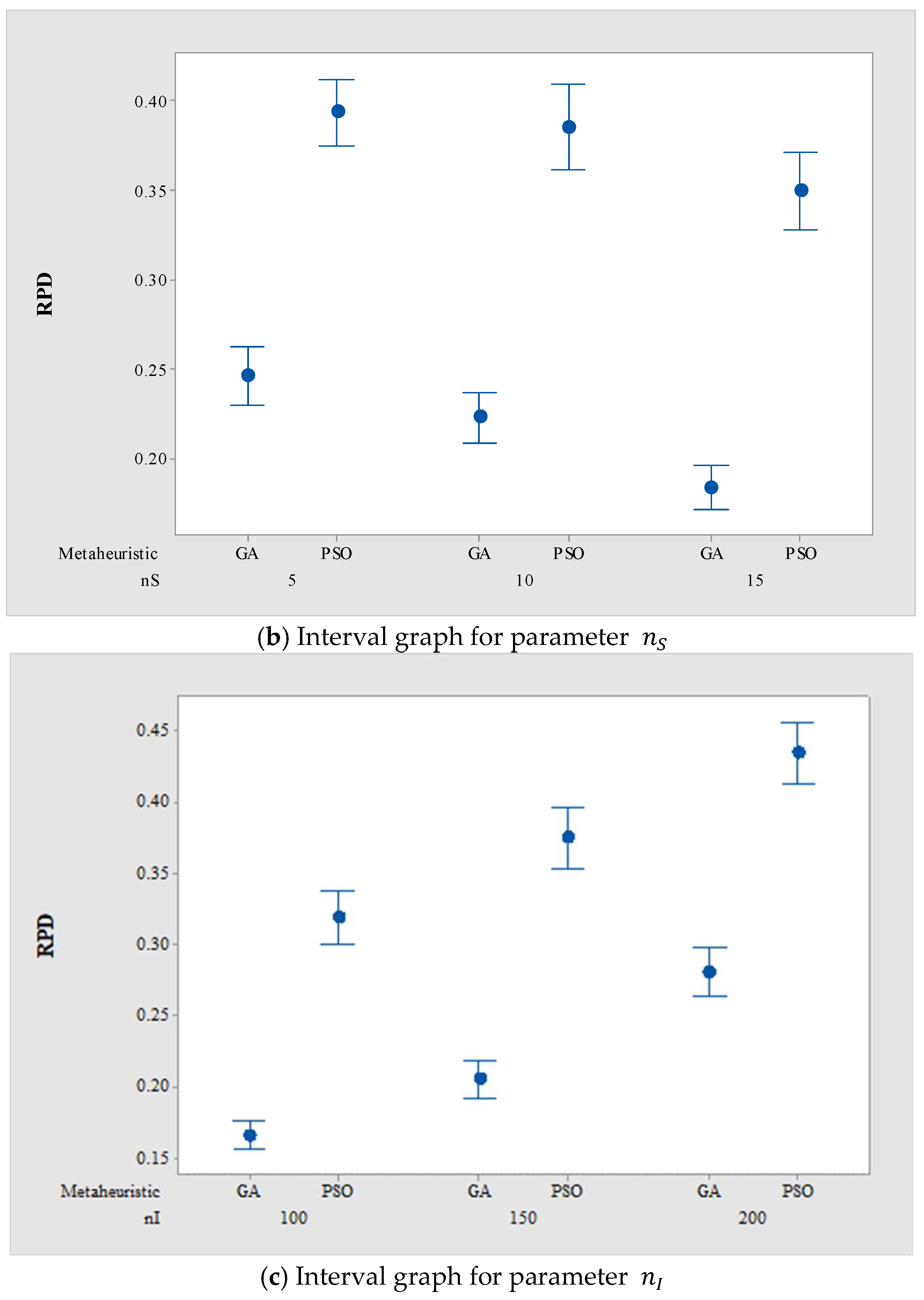
To compare the performance between the GA and PSO, we present confidence interval graphs in Figure 2 and Figure 3. In Figure 2, we show interval graphs for the results of the large-sized experiment with a 0.05 confidence level. As shown in Figure 2, the confidence intervals of the GA and PSO do not overlap. Furthermore, the GA shows a lower mean RPD value and a narrower confidence interval than PSO. We present confidence interval graphs for experimental parameters  n F n S , and  n I  in Figure 3. For graphs in Figure 3a–c, the GA shows smaller mean RPD values and confidence intervals than PSO even when parameters change. Figure 2 and Figure 3 indicate that the GA has a statistically significant difference in performance compared to PSO. In addition, the GA and PSO show larger mean RPD values and confidence intervals as  n I  increases in Figure 3c. It implies that  n I  is the experimental parameter that most affects the complexity of the addressed problem.
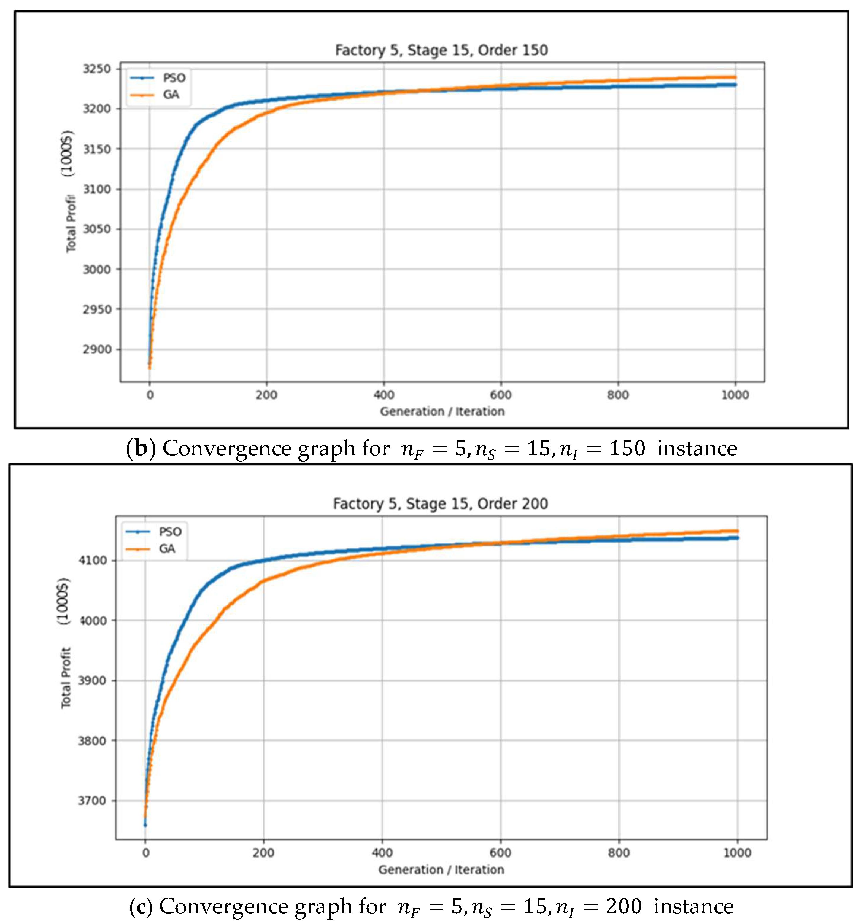
To analyze the convergence of the GA and PSO based on changes in  n I , we address average convergence graphs in Figure 4. We present the convergence graphs when  n F  and  n S  are 5 and 15, respectively. As shown in graphs (a)–(c) of Figure 4, PSO converges faster than the GA in the early stage of the search. However, the GA ultimately outperforms PSO through the continuous improvement of the solution. It implies that genetic and evolutionary operators of the enable the search for a more spacious solution space and continuously improve the solution. In contrast, PSO appears to converge quickly, potentially getting trapped in a local optimum. In addition, the intersection points of the GA and PSO are right-shifted with increasing  n I . This indicates that increasing  n I  requires more search steps to sufficiently converge the performance of the GA and PSO. From the results of the large-sized experiment, Figure 2, Figure 3 and Figure 4, the GA statistically outperforms PSO.

5.3. Results of Sensitivity Analysis

To observe the relationship among order selection, revenue, and order tardiness cost, we conduct sensitivity analysis with the GA. We re-test the large-sized experiments described in Section 5.1 and define the scaling parameter of tardiness costs,  α , as 0.01. To confirm the reason for the order selection, we analyze a relationship between the slack and revenue of the order. We calculate the slack of each order  i S L i , and the relative gap of the  S L i G A P S L i  as follows:
S L i = max D i m e d s S P T s i f , 0
G A P S L i % = max j I S L j S L i max j I S L j × 100
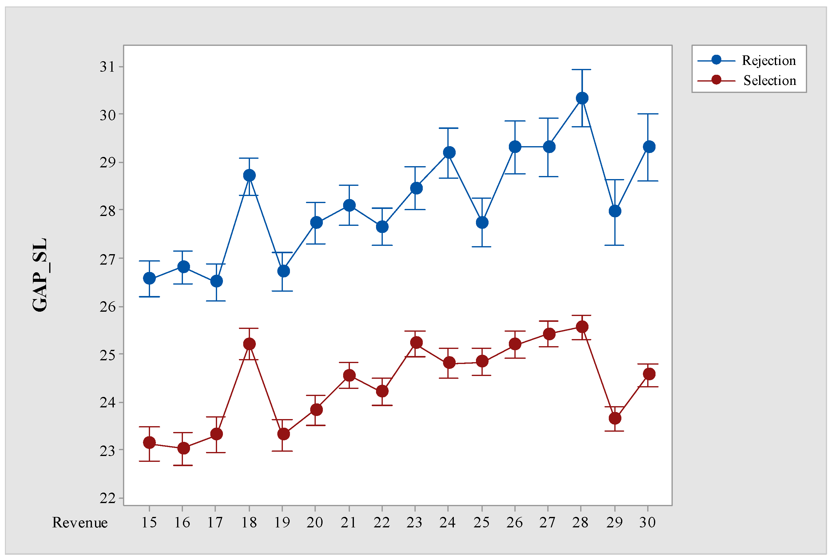
Figure 5 shows the interval graphs of  G A P S L i  according to the revenue of the order  i . The blue and red graphs indicate the interval graphs for the rejected and selected orders, respectively. For each revenue value, we are able to observe that there is no overlap between the blue and red graphs, and the red graph shows a lower mean value than the blue graph. It indicates that the orders with sufficient slacks are statistically significantly selected regardless of the revenue of the order to reduce the potential order tardiness costs.
To observe the relationship between revenue and order tardiness cost, we analyze the relative gap of the tardiness of selected order  i G A P T i , and manufacturing completion time of selected order  i G A P C i , which are calculated as
G A P T i   ( % ) = max j I T j T i max j I T j × 100
G A P C i   % = max j I C j C i max j I C j × 100
where  C i  and  T i  are the manufacturing completion time and tardiness of selected order  i .
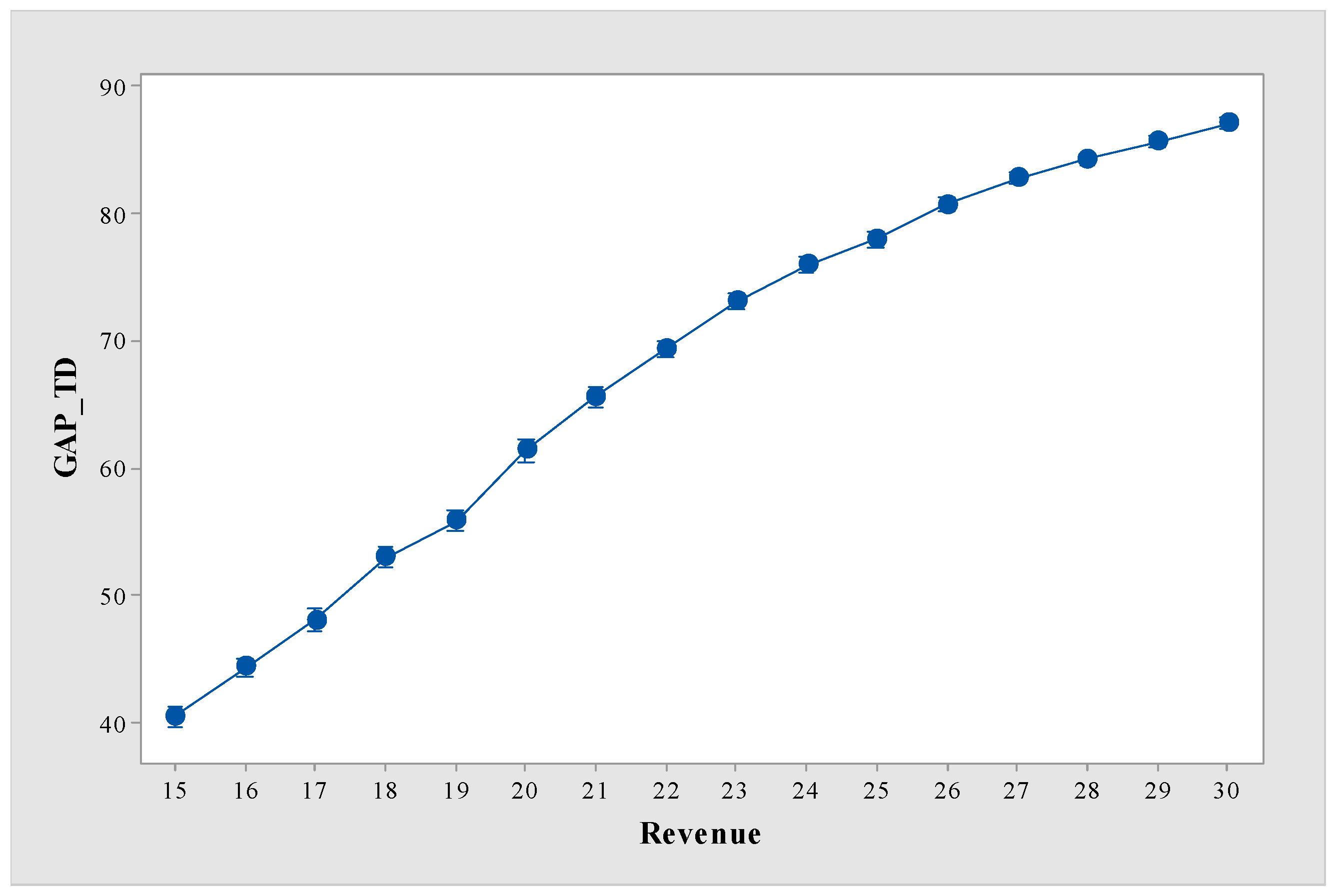
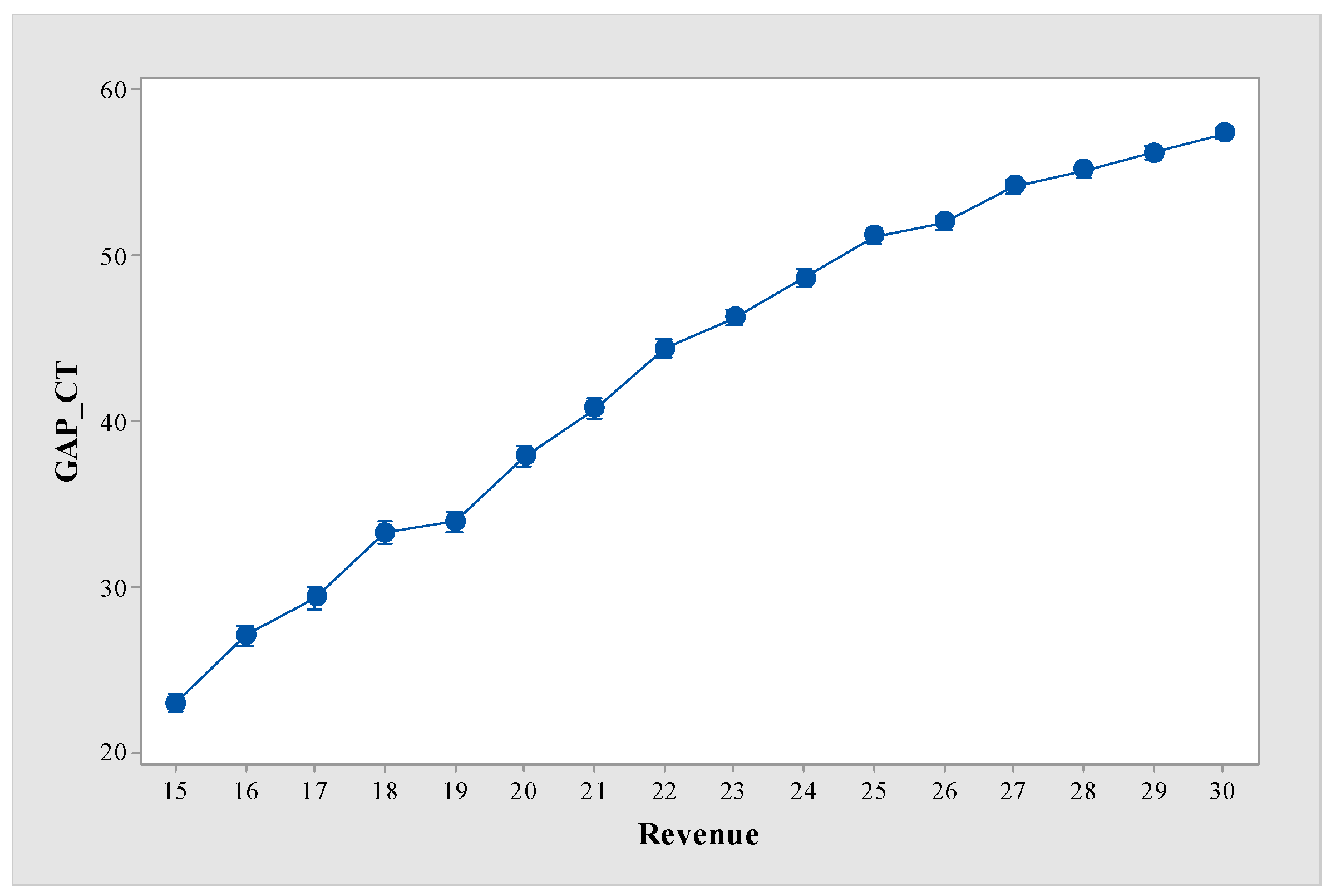
Figure 6 and Figure 7 show the interval graphs of  G A P T i  and  G A P C i  according to the revenue of order  i , respectively. In both Figure 6 and Figure 7, we are able to observe the increasing mean values of  G A P T i  and  G A P C i  as the revenue of the order increases. It indicates that the orders with high revenue are produced before the orders with low revenue are produced to minimize the actual order tardiness costs.
Based on the results of the sensitivity analysis, we are able to suggest managerial insights for the selection of production orders and the sequencing of the assigned orders in each factory. To reduce the potential order tardiness costs, we have to determine the order selection by considering orders with sufficient slack among orders with equal revenue. Furthermore, we have to determine the manufacturing sequence by considering the related revenue to minimize the actual order tardiness costs.

6. Conclusions

We addressed the DPFSP-OAHF that firstly considered distributed heterogeneous permutation flowshop, sequence-dependent setup times, and order acceptance strategy, simultaneously. To find an optimal solution, we developed the MILP model of the addressed problem. Furthermore, we proposed the GA to effectively and efficiently find a near-optimal solution. We conducted numerical experiments to verify and evaluate the performances of the GA. In the small-sized experiments, we verified the GA by comparing it with the developed MILP model and PSO. We compared the GA with PSO and the BH to evaluate the performance of the GA, and the GA showed a statistically significant RPD value in the large-sized experiments. Through the sensitivity analysis with the proposed GA, we suggest managerial insights for the selection of production orders and the sequencing of manufacturing the assigned orders in each factory.
The limitations of this study are as follows: First, the lead time from the factory to the customer is not considered. Second, it is assumed that there is only one flowshop in each factory. In future studies, this study can be extended to multi-factory and multi-flowshop scheduling problems that include the lead time from the factory to the customer. Finally, there are no experiments with real-world data. We will conduct experiments using real-world data in future studies.

Author Contributions

Conceptualization, S.J.L. and B.S.K.; methodology, S.J.L.; software, S.J.L.; validation, S.J.L. and B.S.K.; formal analysis, S.J.L.; investigation, S.J.L.; writing—original draft preparation, S.J.L.; writing—review and editing, S.J.L. and B.S.K.; visualization, S.J.L.; supervision, B.S.K.; funding acquisition, B.S.K. All authors have read and agreed to the published version of the manuscript.

Funding

This work was supported by the Incheon National University Research Grant in 2023 (Grant number: 2023-0181).

Data Availability Statement

The data are available from the corresponding author on reasonable request.

Conflicts of Interest

The authors declare no conflicts of interest.

Appendix A. Base Heuristic

We propose a base heuristic (BH) to efficiently solve the addressed problem. The proposed BH consists of sorting, assigning, and acceptance/rejection phases. In the sorting phase, production orders are sorted in increasing order based on the priority of the order. The priority of order  i  is equal to  R i / D i . We calculate the priority by referring to a weighted earliness due date (WEDD) rule that shows good performance to minimize total tardiness in the DPFS and permutation flowshop scheduling problem [33,34,35,36,37]. In the second phase, we virtually assign each sorted order  i  to each factory  f  and calculate the tardiness of order  i  at factory  f   T i f . In the acceptance/rejection phases, we reject an order  i  if the tardiness cost is higher than its revenue. Otherwise, we assign order  i  to factory  f  with minimum  T i f . Algorithm A1 of the BH is as follows:
Algorithm A1: Base Heuristic
  Input :   Order   list   L ,   Revenue   of   order   i   R i ,   Due   date   of   order   i   D i ,   Weight   α
Sort  L  in increasing order based on  R i / D i
For  i L
  For  f F
    Let  T i f  as tardiness of order  i  at factory  f
    Virtually assign order  i  to factory  f
    Calculate  T i f
  End For
  If  R i α × R i × min 1 f n F T i f
    Reject order  i
  Else
    Assign order  i  to factory  f = argmin 1 f n F T i f
    Update factory  f
  End If
End For

References

  1. Zhou, L.; Zhang, L.; Laili, Y.; Zhao, C.; Xiao, Y. Multi-task Scheduling of Distributed 3D Printing Services in Cloud Manufacturing. Int. J. Adv. Manuf. Technol. 2018, 96, 3003–3017. [Google Scholar] [CrossRef]
  2. Leng, J.; Zhong, Y.; Lin, Z.; Xu, K.; Mourtzis, D.; Zhou, X.; Zheng, P.; Liu, Q.; Zhao, J.L.; Shen, W. Towards Resilience in Industry 5.0: A Decentralized Autonomous Manufacturing Paradigm. J. Manuf. Syst. 2023, 71, 95–114. [Google Scholar] [CrossRef]
  3. Chang, H.C.; Liu, T.K. Optimisation of Distributed Manufacturing Flexible Job Shop Scheduling by Using Hybrid Genetic Algorithms. J. Intell. Manuf. 2017, 28, 1973–1986. [Google Scholar] [CrossRef]
  4. De Giovanni, L.; Pezzella, F. An Improved Genetic Algorithm for the Distributed and Flexible Job-shop Scheduling Problem. Eur. J. Oper. Res. 2010, 200, 395–408. [Google Scholar] [CrossRef]
  5. Shao, W.; Pi, D.; Shao, Z. Optimization of Makespan for the Distributed No-Wait Flow Shop Scheduling Problem with Iterated Greedy Algorithms. Knowl. Based Syst. 2017, 137, 163–181. [Google Scholar] [CrossRef]
  6. Wang, S.Y.; Wang, L.; Liu, M.; Xu, Y. An Effective Estimation of Distribution Algorithm for Solving the Distributed Permutation Flow-Shop Scheduling Problem. Int. J. Prod. Econ. 2013, 145, 387–396. [Google Scholar] [CrossRef]
  7. Mönch, L.; Shen, L. Parallel Machine Scheduling with the Total Weighted Delivery Time Performance Measure in Distributed Manufacturing. Comput. Oper. Res. 2021, 127, 105126. [Google Scholar] [CrossRef]
  8. Lei, D.; Yuan, Y.; Cai, J.; Bai, D. An Imperialist Competitive Algorithm with Memory for Distributed Unrelated Parallel Machines Scheduling. Int. J. Prod. Res. 2020, 58, 597–614. [Google Scholar] [CrossRef]
  9. Behnamian, J.; Fatemi Ghomi, S.M.T. A Survey of Multi-Factory Scheduling. J. Intell. Manuf. 2016, 27, 231–249. [Google Scholar] [CrossRef]
  10. Bagheri Rad, N.; Behnamian, J. Recent Trends in Distributed Production Network Scheduling Problem; Springer: Berlin/Heidelberg, Germany, 2022. [Google Scholar]
  11. Marin-Garcia, J.A.; Garcia-Sabater, J.P.; Miralles, C.; Villalobos, A.R. Profile and Competences of Spanish Industrial Engineers in the European Higher Education Area (EHEA). J. Ind. Eng. Manag. 2008, 1, 269–284. [Google Scholar] [CrossRef]
  12. Renna, P. Coordination Strategies to Support Distributed Production Planning in Production Networks. Eur. J. Ind. Eng. 2015, 9, 366–394. [Google Scholar] [CrossRef]
  13. Naderi, B.; Ruiz, R. The Distributed Permutation Flowshop Scheduling Problem. Comput. Oper. Res. 2010, 37, 754–768. [Google Scholar] [CrossRef]
  14. Slotnick, S.A. Order Acceptance and Scheduling: A Taxonomy and Review. Eur. J. Oper. Res. 2011, 212, 1–11. [Google Scholar] [CrossRef]
  15. Karabulut, K.; Öztop, H.; Kizilay, D.; Tasgetiren, M.F.; Kandiller, L. An Evolution Strategy Approach for the Distributed Permutation Flowshop Scheduling Problem with Sequence-Dependent Setup Times. Comput. Oper. Res. 2022, 142, 105733. [Google Scholar] [CrossRef]
  16. Huang, J.P.; Pan, Q.K.; Gao, L. An Effective Iterated Greedy Method for the Distributed Permutation Flowshop Scheduling Problem with Sequence-Dependent Setup Times. Swarm Evol. Comput. 2020, 59, 100742. [Google Scholar] [CrossRef]
  17. Zhao, F.; Hu, X.; Wang, L.; Li, Z. A Memetic Discrete Differential Evolution Algorithm for the Distributed Permutation Flow Shop Scheduling Problem. Complex Intell. Syst. 2022, 8, 141–161. [Google Scholar] [CrossRef]
  18. Gogos, C. Solving the Distributed Permutation Flow-Shop Scheduling Problem Using Constrained Programming. Appl. Sci. 2023, 13, 12562. [Google Scholar] [CrossRef]
  19. Yang, S.; Xu, Z. The Distributed Assembly Permutation Flowshop Scheduling Problem with Flexible Assembly and Batch Delivery. Int. J. Prod. Res. 2021, 59, 4053–4071. [Google Scholar] [CrossRef]
  20. Huang, Y.Y.; Pan, Q.K.; Gao, L.; Miao, Z.H.; Peng, C. A Two-Phase Evolutionary Algorithm for Multi-Objective Distributed Assembly Permutation Flowshop Scheduling Problem. Swarm Evol. Comput. 2022, 74, 101128. [Google Scholar] [CrossRef]
  21. Pan, Y.; Gao, K.; Li, Z.; Wu, N. Improved Meta-Heuristics for Solving Distributed Lot-Streaming Permutation Flow Shop Scheduling Problems. IEEE Trans. Autom. Sci. Eng. 2023, 20, 361–371. [Google Scholar] [CrossRef]
  22. Luo, C.; Gong, W.; Li, R.; Lu, C. Problem-Specific Knowledge MOEA/D for Energy-Efficient Scheduling of Distributed Permutation Flow Shop in Heterogeneous Factories. Eng. Appl. Artif. Intell. 2023, 123, 106454. [Google Scholar] [CrossRef]
  23. Meng, T.; Pan, Q.K. A Distributed Heterogeneous Permutation Flowshop Scheduling Problem with Lot-Streaming and Carryover Sequence-Dependent Setup Time. Swarm Evol. Comput. 2021, 60, 100804. [Google Scholar] [CrossRef]
  24. Khare, A.; Agrawal, S. Effective Heuristics and Metaheuristics to Minimise Total Tardiness for the Distributed Permutation Flowshop Scheduling Problem. Int. J. Prod. Res. 2021, 59, 7266–7282. [Google Scholar] [CrossRef]
  25. Lin, Z.; Jing, X.L.; Jia, B.X. An Iterated Greedy Algorithm for Distributed Flowshops with Tardiness and Rejection Costs to Maximize Total Profit. Expert Syst. Appl. 2023, 233, 120830. [Google Scholar] [CrossRef]
  26. Zhang, Q.; Zhen, T. Improved Jaya Algorithm for Energy-Efficient Distributed Heterogeneous Permutation Flow Shop Scheduling. J. Supercomput. 2025, 81, 434. [Google Scholar] [CrossRef]
  27. Song, H.; Li, J.; Du, Z.; Yu, X.; Xu, Y.; Zheng, Z.; Li, J. A Q-learning Driven Multi-Objective Evolutionary Algorithm for Worker Fatigue Dual-Resource-Constrained Distributed Hybrid Flow Shop. Comput. Oper. Res. 2025, 175, 106919. [Google Scholar] [CrossRef]
  28. Zhu, N.; Zhao, F.; Yu, Y.; Wang, L. A Cooperative Learning-Aware Dynamic Hierarchical Hyper-Heuristic for Distributed Heterogeneous Mixed No-Wait Flow-Shop Scheduling. Swarm Evol. Comput. 2024, 90, 101668. [Google Scholar] [CrossRef]
  29. Perez-Gonzalez, P.; Framinan, J.M. A Review and Classification on Distributed Permutation Flowshop Scheduling Problems. Eur. J. Oper. Res. 2023, 312, 1–21. [Google Scholar] [CrossRef]
  30. Mraihi, T.; Driss, O.B.; El-Haouzi, H.B. Distributed Permutation Flow Shop Scheduling Problem with Worker Flexibility: Review, Trends and Model Proposition. Expert Syst. Appl. 2023, 238, 121947. [Google Scholar] [CrossRef]
  31. Kapadia, M.S.; Uzsoy, R.; Starly, B.; Warsing, D.P. A Genetic Algorithm for Order Acceptance and Scheduling in Additive Manufacturing. Int. J. Prod. Res. 2021, 60, 1–18. [Google Scholar] [CrossRef]
  32. Kan, A.R. General Flow-Shop and Job-Shop Problems. In Machine Scheduling Problems; Springer: Boston, MA, USA, 1976; pp. 106–130. [Google Scholar]
  33. Pan, Q.K.; Tasgetiren, M.F.; Liang, Y.C. A Discrete Particle Swarm Optimization Algorithm for the No-Wait Flowshop Scheduling Problem. Comput. Oper. Res. 2008, 35, 2807–2839. [Google Scholar] [CrossRef]
  34. Marini, F.; Walczak, B. Particle Swarm Optimization (PSO). A Tutorial. Chemom. Intell. Lab. Syst. 2015, 149, 153–165. [Google Scholar] [CrossRef]
  35. Cerveira, M.I.F. Heuristics for the Distributed Permutation Flowshop Scheduling Problem with the Weighted Tardiness Objective. 2019. Available online: https://www.proquest.com/openview/109fa27057466f781cfeac17a0b99ee1/1?pq-origsite=gscholar&cbl=2026366&diss=y (accessed on 3 March 2025).
  36. Ruiz, R.; Stützle, T. An Iterated Greedy Heuristic for the Sequence Dependent Setup Times Flowshop Problem with Makespan and Weighted Tardiness Objectives. Eur. J. Oper. Res. 2008, 187, 1143–1159. [Google Scholar] [CrossRef]
  37. Molina-Sánchez, L.P.; González-Neira, E.M. GRASP to Minimize Total Weighted Tardiness in a Permutation Flow Shop Environment. Int. J. Ind. Eng. Comput. 2016, 7, 161–176. [Google Scholar] [CrossRef]
Figure 1. An Example of solution representations, decoding procedures, and scheduling results for the proposed GA and PSO ((a) Encoded solution structure; (b) Result of the order selection and factory assignment; (c) Gantt-chart of each factory; S1, S2, and S3 in subfigure (c) means the stage 1, 2, and 3, respectively; The numbers in the boxes in subfigure (c) indicate processing time).
Mathematics 13 00877 g001
Figure 2. Interval graph showing statistically significant differences in RPD values of GA and PSO (blue dots means the average value).
Mathematics 13 00877 g002
Figure 3. Interval graph showing statistically significant differences in the RPD values of the GA and PSO for parameters  n F n S , and  n I  ((a) Interval graph for parameter  n F ; (b) Interval graph for parameter  n S ; (c) Interval graph for parameter  n I ; Blue dots means the average value).
Mathematics 13 00877 g003aMathematics 13 00877 g003b
Figure 4. Convergence graph for instance.
Mathematics 13 00877 g004aMathematics 13 00877 g004b
Figure 5. Interval graph for  G A P S L i .
Mathematics 13 00877 g005
Figure 6. Interval graph for  G A P T i  (blue dots means the value of  G A P T i ).
Mathematics 13 00877 g006
Figure 7. Interval graph for  G A P C i  (blue dots means the value of  G A P C i ).
Mathematics 13 00877 g007
Table 1. Literature survey.
OAFrameworkSetupEtc.MethodObjective
HomoHeteroEtc.SDSI
[16] Mathematical model, IGRMin.  C m a x
[15] MILP, CP, ES_enMin.  C m a x
[17] MMDEMin.  C m a x
[18] Heuristic, CP Min.  C m a x
[19] Assembly factories Batch DeliveryHeuristic, VND, IGMin. DTC
[20] Assembly line TEAMin. {TF, TT}
[21] Lot-StreamingMathematical model, GA, PSO, ABC, HS, JayaMin.  C m a x
[22] KMOEA/DMin. { C m a x , T E C }
[23] Lot-streamingMILP, Constructive Heuristic, NEABCMin.  C m a x
[24] MILP, HHO, IGMin. TD
[25] DeadlineMILP, IG_TRMax. Total profit
[26] JayaMin. { C m a x , TEC}
[27] Worker
fatigue
Q-learning driven multi-objective evolutionary algorithmMin.  C m a x
[28] No-waitHyper-heuristicMin.  C m a x
This MILP, GA, PSOMax. Total profit
Homo: homogeneous; Hetero: heterogeneous; SD: sequence-dependent; SI: sequence-independent, TEC: total energy consumption.
Table 2. Design of experiments.
Small-Sized
Instances
Large-Sized
Instances
  n F 3, 45, 6, 7
  n S 3, 45, 10, 15
  n I 8, 10, 12100, 150, 200
  R i u n i f 15 , 30  (1000 $)
  D i n S × m e d C O i j f s + m e d s S P T s i f × 1 + r 2 n F  (min)
  P T s i f u n i f 2 , 5  (min)
  C O i j f s u n i f 2 , 5  (min)
  α 0.010.001
Fitness
Measure
  R P D = Z b e s t Z Z b e s t × 100 %
Table 3. Result of small-sized experiments.
Ins.   n F   n S   n I   Z b e s t MILPPSOGA
RPDCPURPDCPURPDCPU
1338173.00173.000.380.302.010.002.57
2 10219.40219.4081.891.992.260.542.97
3 12228.10228.101800++4.542.322.632.98
4 48181.00181.000.190.002.300.002.92
5 10239.00239.000.380.002.680.003.35
6 12265.00265.0065.612.832.901.873.60
7438175.00175.000.470.002.090.002.74
8 10232.00232.002.950.002.410.003.11
9 12266.80266.801800++3.292.721.953.42
10 48184.00184.000.230.002.450.003.13
11 10228.00228.000.450.002.850.003.57
12 12302.00302.004.340.003.220.004.03
Mean224.44313.091.082.520.583.20
Table 4. Result of large-sized experiment.
Ins.   n F   n S   n I   Z b e s t BHPSOGA
RPD CPU RPD CPU RPD CPU
1551002085.2858.54<0.010.4351.160.1860.14
2 1503117.1173.51<0.010.5076.090.2488.90
3 2004089.5079.56<0.010.52100.320.31117.30
4 101002141.0052.19<0.010.5088.110.2599.32
5 1503199.0866.30<0.010.52130.910.22147.78
6 2004057.9675.97<0.010.67173.420.34195.25
7 151002110.5641.32<0.010.47124.580.20138.82
8 1503247.7963.01<0.010.56184.350.25206.29
9 2004158.5371.23<0.010.51246.160.21273.49
10651002199.8649.42<0.010.3352.120.1961.29
11 1503094.2467.66<0.010.4577.010.2490.54
12 2004158.0976.40<0.010.41101.810.29119.55
13 101002134.0638.61<0.010.3088.970.13100.68
14 1503265.7160.56<0.010.34132.080.20149.32
15 2004132.8270.42<0.010.41175.080.29197.79
16 151002285.3930.82<0.010.25124.520.16140.00
17 1503263.9454.20<0.010.27186.840.10208.31
18 2004289.7165.40<0.010.43247.830.28276.32
19751002246.7639.55<0.010.1952.830.1062.43
20 1503267.9161.30<0.010.3278.120.2792.08
21 2004233.8572.09<0.010.39103.200.40122.14
22 101002301.3728.26<0.010.2389.610.17101.81
23 1503244.5454.28<0.010.18133.150.17151.24
24 2004229.2567.08<0.010.33176.520.24200.70
25 151002230.9422.31<0.010.18126.080.12141.21
26 1503301.4845.13<0.010.24186.800.17210.39
27 2004261.6060.05<0.010.24252.750.16279.27
Mean3198.0957.23<0.010.38131.870.22149.35
Disclaimer/Publisher’s Note: The statements, opinions and data contained in all publications are solely those of the individual author(s) and contributor(s) and not of MDPI and/or the editor(s). MDPI and/or the editor(s) disclaim responsibility for any injury to people or property resulting from any ideas, methods, instructions or products referred to in the content.