A Column-Generation-Based Exact Algorithm to Solve the Full-Truckload Vehicle-Routing Problem

Abstract

This study addresses a specialized variant of the full-truckload delivery problem inspired by a Turkish logistics firm that operates in the liquid transportation sector. An exact algorithm is proposed for the relevant problem, to which no exact approach has been applied before. Multiple customer and trailer types, as well as washing operations, are introduced simultaneously during the exact solution process, bringing new aspects to the exact algorithm approach among full-truckload systems in the literature. The objective is to minimize transportation costs while addressing constraints related to multiple time windows, trailer types, customer types, product types, a heterogeneous fleet with limited capacity, multiple departure points, and various actions such as loading, unloading, and washing. Additionally, the elimination or reduction of waiting times is provided along transportation routes. In order to achieve optimal solutions, an exact algorithm based on the column generation method is proposed. A route-based insertion algorithm is also employed for initial routes/columns. Regarding the acquisition of integral solutions in the exact algorithm, both dynamic and static sets of valid inequalities are incorporated. A label-setting algorithm is used to generate columns within the exact algorithm by being accelerated through bi-directional search, ng-route relaxation, subproblem selection, and heuristic column generation. Due to the problem-dependent structure of the column generation method and acceleration techniques, a tailored version of them is included in the solution process. Performance analysis, which was conducted using artificial input sets based on the real-life operations of the logistics firm, demonstrates that optimality gaps of less than 1% can be attained within reasonable times even for large-scale instances relevant to the industry, such as 120 customers, 8 product and 8 trailer types, 4 daily time windows, and 40 departure points.

1. Introduction

In today’s world, people and organizations are living in vast interconnected networks and the importance of transportation within these networks is growing dramatically. Vehicle-routing problems (VRP) constitute a significant proportion of these network challenges due to their critical role in the logistics sector. Insufficient fleet management or inaccurate calculations may culminate in substantial financial losses and impinge on many organizations within the supply chain. Therefore, sustainable and efficient transportation systems have become essential in the modern era.

The liquid transportation company that has inspired our problem has the largest fleet among Turkish logistics companies with 600 trucks. Due to the high volume of customer demands, consisting of contracted and non-contracted ones, they deploy both owned and rented trucks to meet service needs. In short, their operations consistently involve large-scale instances. The company endeavors to cover a wide variety of demands having a higher number of product types compared to its competitors in the sector. Thus, a diverse range of trailer types is utilized to manage these distinct product categories at the same time. However, frequent washing operations are also required to avoid contamination. Due to the fact that their operations impose an enormous number of decisions posing great difficulties for the company, a problem-specific exact algorithm is imperative.

Given the complexity of logistics operations, the VRP encompasses numerous variants (see Konstantakopoulos et al. [1] for an extensive review), necessitating the development and implementation of problem-specific solutions. One variant of the VRP is full-truckload (FTL) operations, in which large shipments require the full capacity of a truck. Currently, FTL operations may involve the transportation of containers from ports to production facilities, the delivery of cement to construction sites, debris removal from construction sites or mining sites, and liquid transportation. Furthermore, the application of FTL principles can be examined in the healthcare sector. For instance, an ambulance fleet departing from multiple locations may need to pick up patients at specific points and transport them to hospitals, minimizing the total time spent by vehicles rather than transportation costs due to the urgency of the situation.

This study addresses a specialized FTL problem inspired by the operations of a prominent Turkish logistics firm that engages in liquid transportation with 600 trucks. In many of their activities, a network is involved where a limited number of rented and owned vehicles remain idle at multiple departure points and are ready to return to the garage by being equipped with various types of trailers. Simultaneously, these vehicles may be assigned to transport products from supply points (loading zones) to customer locations (unloading zones), and designated vehicles serving customer locations must return to the terminal/garage point after completing their routes. Vehicles must adhere to time window constraints specified for those zones. Furthermore, in order to accommodate the transportation of different product types, vehicles are entailed to visit washing centers to clean their trailers, ensuring readiness for the next load. During the switch between two product types, the washing process must be performed according to the washing matrix, which outlines the required washing times. Vehicles also transport products in trailers that conform to a trailer–product matrix specifying which product types are compatible with which trailer types. In the logistics market, orders originating from contracted customers are mandatory and must be prioritized while optional orders from non-contracted customers arise occasionally. Thus, the primary objective is to optimize routing for the current fleet by minimizing overall transportation costs and eliminating or reducing waiting times at visited nodes.

The incorporation of multiple time windows, departure nodes, diverse customer types, a heterogeneous fleet, and washing operations significantly increases the number of decision variables for logistics firms. These factors considerably contribute to route complexity or route combination, making the optimal vehicle decisions exceedingly challenging. Suboptimal decisions among those combinations may lead to high fixed or variable costs of vehicles and unsatisfied customers. Thus, a logistics firm may experience a massive loss of profits, market shares, and demands, being deprived of competitiveness against its rivals.

Due to the significant complexity of VRP, numerous heuristic algorithms, such as genetic algorithms (Holland [2]), ant colony algorithms (Dorigo et al. [3]), large neighborhood search algorithms, and tabu search algorithms (Glover [4]), are widely used to generate initial solutions and improve them accordingly. However, these algorithms were not designed to guarantee optimality. Instead, they just provide upper-bound solutions.

Exact algorithms are used in VRP less frequently than heuristic methods. Their application to FTL problems is even more uncommon since the FTL variant has been studied less extensively within the VRP domain. In this study, both exact algorithm structures and heuristic methods are integrated to address the specified FTL problem. A modified route-based insertion heuristic (Solomon [5]) is utilized to generate initial routes/columns providing a starting point for an exact algorithm based on the column generation (CG) method inspired by Dantzig and Wolfe [6].

In order to enhance the exact algorithm, valid inequalities, such as arc flow inequalities (Costa, Contardo, and Desaulniers [7]) and k-path inequalities (Desaulniers, Lessard, and Hadjar [8]), are incorporated. These inequalities strengthen the CG algorithm by generating promising routes through the use of diverse dual variables. Additionally, four acceleration techniques are deployed to expedite the process. The first acceleration technique, introduced by Righini and Salani [9], employs a bi-directional search within the label-setting algorithm to accelerate the solution of the elementary shortest path problem with resource constraints (ESPPRCs). The second technique uses ng-route relaxation, developed by Baldacci, Mingozzi, and Roberti [10], allowing the inclusion of non-elementary paths alongside elementary ones in the relaxed -master problem (RMP) of the CG algorithm. The third technique focuses on subproblem selection to prioritize the identification of subproblems that are likely to contain promising columns/routes. While it is primarily heuristic, this technique can evaluate all subproblems when necessary. The final technique involves a heuristic column generator inspired by Desaulniers et al. [8], which identifies the first promising column encountered within the given subproblem. When it is required, this approach can also systematically evaluate all possible routes to ensure comprehensive exploration.

To sum up, a relevant FTL transportation network structure that has been widely encountered in the logistics market was analyzed by considering the important aspects of VRP in both literature and real life. Therefore, our contributions can be expressed as follows:

• This study addresses various characteristics simultaneously, such as multiple time windows, departure points, product types, trailer types, a heterogeneous fleet, and a limited number of vehicles at each departure point within the FTL network, distinguishing itself from other studies in the literature.
• This study uniquely incorporates washing operations for trailers to facilitate product changeovers during liquid transportation. Additionally, it integrates washing costs and washing times within the FTL network.
• The integration of the CG method, designed to solve the problem exactly, was uniquely implemented in this study, taking the distinctive aspects of the problem into account. For instance, the label-setting algorithm used for CG was specifically adapted to the FTL network, which is the focus of this research.
• Acceleration techniques such as ng-route relaxation and bi-directional search mechanism were uniquely modified to align with the specific characteristics of the FTL network considered in this study.
• The study includes a comprehensive performance analysis of the exact algorithm across a wide range of instances for the specified FTL structure.

The remainder of this paper is organized as follows: Section 2 presents a detailed literature review with a particular focus on FTL transportation systems. Section 3 introduces the problem definition, mathematical model, and network representation. Subsequently, Section 4 elaborates on the construction heuristic procedures, CG method, and the associated acceleration techniques. In Section 5, the computational performance results of the proposed exact approach are presented with respect to problem instances. Finally, Section 6 provides concluding remarks and discusses potential future research directions.

2. Literature Review

It should be noted that research on FTL systems is relatively scarce in the literature. While a limited number of studies delve into the specifics of the FTL concept, its operations are evident in many critical areas. These studies predominantly focus on problem-specific heuristic algorithms, whereas solutions based on exact algorithms remain uncommon. Recently, machine learning, deep learning, and agent-based techniques have been applied to the VRP. However, studies integrating heuristic or learning algorithms or agent-based techniques with exact algorithm enhancements are still notably underrepresented. Therefore, in our study, we aim to solve our specified FTL problem encompassing both exact and heuristic algorithms with relevant acceleration techniques.

The FTL problem was first introduced by Ball et al. [11] and aimed to find the optimal fleet size obtaining vehicle routes while satisfying maximum route-time restrictions. They managed to formulate the problem and described some approximate solution strategies discussing important implementation issues. Then, Desrosiers et al. [12] used an asymmetrical traveling salesman problem with two types of restrictions in order to present an effective approach to FTL systems.

The literature actually contains a wealth of heuristic algorithms applied to FTL problems, and researchers continue to favour these approaches due to their ease of implementation and low computational complexity. Agent-based simulations are also appealing for tackling complicated FTL operations.

Soleilhac et al. [13] studied the VRP involving both FTL and less than truck load (LTL) shipments. Their objective was to identify the optimal combination of FTL and LTL shipments to minimize transportation costs. They proposed a large neighborhood search heuristic algorithm to manage the computational complexity. Ghilas et al. [14] focused on the tendering process related to FTL transportation and used a tailored adaptive large neighborhood search to overcome the computational issues created by the problem. El Bouyahyiouy [15] investigated the selective FTL system with multi-depot and time windows. A formulation based on mixed-integer modeling was provided, and a genetic algorithm was also created for comparison. Ghorpade et al. [16] proposed an order-first split-second heuristic for an alternative routing strategy for freight railways, modeling the system according to pickup and delivery with customer-specified origin and destination and multiple FTL demands by each customer. Fadda et al. [17] analyzed port visitation with a heterogeneous fleet including vessels and small ships. While their work resembled FTL and LTL operations, they focused on maritime transport instead of trucks. A mixed-integer model with problem-specific valid inequalities was developed to achieve optimality, and a large neighborhood search heuristic was applied to solve large-scale instances efficiently. Çabuk, Selin, and Rızvan Erol [18] examined a specific problem characterized by stochastic conditions on the management of FTL operations. A dynamic optimization approach was embraced, incorporating intelligent-agent-based modeling to assign vehicles and determine their routes. Door-to-door deliveries are becoming widespread in populations. Thus, Lu et al. [19] employed a crowdsource delivery model to overcome uncertainties utilizing bounded rationality. The whale optimization algorithm was also combined with that model to design an effective heuristic.

The literature contains relatively few studies focusing on exact algorithms for FTL transportation. Most approaches employ mixed-integer linear programming (MILP) models. In order to solve large-scale instances, valid inequalities, branch and bound, or branch and cut algorithms are commonly utilized. However, CG-based methods have been applied to FTL systems less frequently.

Masmoudi et al. [20] addressed container truck transportation based on FTL operations involving a mixed-fleet heterogeneous dial-a-ride problem. They developed a MILP method to minimize transportation costs and reduce the associated environmental impact. Nasr et al. [21] studied the agri-fresh food supply chain between farmers and markets where FTL and LTL transportations can take place. A MILP model was developed for small-scale instances, while Lagrange relaxation and the genetic algorithm were used in large-scale ones. However, these two previous works did not include the CG method, which is considerably effective in large-scale instances of VRP as opposed to our work. Aickelin et al. [22] proposed a hybrid pricing and cutting approach for the multi-shift FTL VRP. They combined CG techniques with metaheuristics to achieve satisfactory solutions. However, their study lacks extremely efficient and widely used acceleration techniques, such as bi-directional search and ng-route relaxation, with respect to the CG method in VRP as opposed to our work. Baller et al. [23] studied the automotive inbound logistic problem in which transportations should be handled with LTL or FTL or express services. A scalable MILP method was deployed, bringing along problem-specific valid inequalities to find the exact solution more effectively. Bellabdaoui and El Bouyahyiouy [24] focused on the FTL-routing problem, aiming to maximize the total profit generated by trucks during their return journeys under time window constraints. They employed a genetic algorithm to identify feasible routes followed by a MILP model to determine the optimal sequence of commodities for each truck route. Melchiori, Luciana, et al. [25] studied resource synchronization in an FTL problem using an exact algorithm based on integer linear programming (ILP). Symmetry-breaking cuts and additional valid inequalities were also included to be effective in large-scale instances. Bouyahyiouy et al. [26] investigated a lexicographic approach for the robust selective FTL problem using a MILP-based algorithm under operational constraints to minimize transportation costs. These previous four studies only involve loading and unloading operations without any other actions, such as washing, while they are devoid of a significantly effective CG method and its acceleration techniques in contrast to our study.

According to the literature, our work distinguishes itself from pure heuristic-based FTL studies by having a prominent exact algorithm. Nevertheless, studies that have an exact algorithm can achieve solving at most medium-scale instances. Therefore, they always resort to heuristics when addressing the large-scale ones. Undoubtedly, there are very few FTL studies that focused on the CG method in large-scale instances efficiently. However, our FTL network structure and problem concept are notably distinct and unique, requiring a unique design and implementation of the CG method. This is due to the inherently problem-dependent nature of the CG method, which tends to vary significantly based on the specific characteristics of the problem.

3. Problem Description

3.1. Problem Definition

This study aims to provide an exact solution for an FTL delivery vehicle-scheduling problem. The problem involves multiple departure points/nodes and a single terminal point/node, multiple time window constraints, a limited number of vehicles, different types of vehicles and trailers, distinct product types, and a mix of selective (non-contracted) and non-selective (contracted) customers. Contracted customers’ demands must be fulfilled, whereas non-contracted customers’ demands may remain unmet if serving them does not contribute to a reduction in overall costs. With respect to multiple time windows of a relevant node, each represents a distinct time interval that is completely separated from other intervals of that node. If a vehicle arrives at a loading or unloading zone earlier than the specified time window, it must wait until the window opens to begin service. Conversely, if the vehicle arrives later, the visit in that time window becomes infeasible for that vehicle. Additionally, logistics companies may consolidate demands for subsequent service to achieve lower costs because incorporating multiple time windows of supply (loading zones) and customer nodes (unloading zones) increases the number of feasible route combinations for the satisfaction of customers without violating their deadlines. For instance, customers may ask to be satisfied in at most three or four days. That is why our work involves daily based multiple time windows.

In addition, FTL networks often include vehicles that have been stationed in multiple departure areas with a connected trailer after the completion of their previous routes resulting from previous orders. These idle vehicles introduce further complexity to the problem since decisions must be made regarding the departure locations. The problem also includes a limited number of vehicles categorized into two distinct types and assigned to each departure point. In FTL logistics, companies commonly rent vehicles in addition to their own fleet to alleviate costs. Nevertheless, despite the cost savings, logistics companies must maintain their owned fleet to reduce reliance on external providers. Thus, the efficient utilization of the entire fleet is a serious challenge and critical for achieving optimal costs.

Product compatibility is another vital consideration in FTL deliveries. Our work was inspired by the practices of a local logistics company that has specialized in liquid transportation. Therefore, trailers in the study are capable of transporting different types of products, requiring preparation to prevent any contamination during liquid transportation. Otherwise, contamination would decrease the quality of the product and create displeasure between the logistics firm and its customers. For this reason, washing centers are incorporated into the problem, and trailers should comply with the structure of the relevant trailer–product matrix and washing matrix. The trailer–product matrix indicates which trailers can carry which products, while the washing matrix specifies the time required to clean a trailer after unloading one product type and before loading another type. For instance, if a rented vehicle is equipped with a trailer that can transport both oil and acid, and the vehicle is scheduled to load acid after unloading oil, then that trailer must undergo a washing process to ensure adequate preparation for the new load. Furthermore, compartmentalization is mostly forbidden because of safety issues. Loaded liquid types with distinct densities tend to deteriorate the weight distribution on the vehicle, disrupting the weight–volume balance. According to road regulations, a vehicle should avoid stability issues. Additionally, some liquid types may be so hazardous that vehicles may be required to travel along different routes that do not pose a threat to the environment during accidents. Even bridge selection becomes significant during transportation. Process time of loading and unloading times for liquid products also tend to change uniquely due to liquid viscosity or pumping capacity. For instance, highly inflammable liquids are preferred to be pumped slowly to reduce the friction effect, avoiding any explosion.

Moreover, FTL deliveries always involve loading and unloading locations, corresponding to supply and demand points, respectively. In this study, demand points refer to customer points since demands are met at those points, whereas supply points represent entities that request the logistics company to transport products to their customers. Hence, unloading zones or demand points are associated with customer points, and loading zones refer to supply points throughout this work.

Lastly, the minimization of redundant waiting times is one of the significant challenges for logistic firms. For example, adjusting the departure time of a vehicle to allow it to leave the departure node later can eliminate or decrease the redundant waiting times at nodes on the potential route without affecting the overall route cost. This ensures more efficient route execution and better utilization of resources such as time.

The objective, as outlined in the problem description, is to minimize the total transportation cost while maintaining a low optimality gap within reasonable computational times and ensuring optimal routing for the relevant vehicles with reduced or eliminated waiting times at the visited nodes.

Based on the aforementioned definition, basic characteristics of the relevant FTL problem can be summarized as follows:

• The transportation network consists of washing nodes, multiple departure nodes, a terminal/garage node, supply nodes, and demand nodes.
• For each product type, there is one supply node and multiple demand nodes
• There are multiple time windows for both supply nodes/loading zones and demand nodes/unloading zones
• Vehicles have two different types; they are either rented or owned by the logistics firm
• Certain types of trailers can be used to transport specified products
• Whenever a trailer is required to carry a different product type, a washing process takes place, imposing washing costs and washing time

Throughout the problem and execution of algorithms that will be explained in the Methodology Section, the following are assumed:

• Environmental factors, such as congestion or accidents, are ignored.
• Multiple time windows are separated and limited.
• Time windows are consecutive and daily based.
• There is a limited number of owned and rented vehicles at each departure point.
• Arc costs and washing costs are predetermined.
• Certain revenues exist for the selection of a non-contracted customer.
• Loading at supply points and unloading at customer points can only occur.
• Trailers are identical except for their ability to carry distinct products.
• The arc cost for a loaded vehicle is two times higher than an unloaded one.
• A predetermined number of washing centers, supply points, customer points, and departure points are included.
• Predetermined travel times and washing times exist.
• The trailer–product matrix and washing matrix structures remain constant and predetermined.
• A certain number of product types and trailer types are included.

Undoubtedly, accidents may happen and compel the logistics firm to take instant actions using real-time optimization concepts (which are irrelevant to our work) that mostly consist of agent-based modeling. However, those do not occur frequently in real life scenarios. Nevertheless, FTL-based logistics firms, which mostly need to deal with changing types of customer, do not schedule over a long time horizon due to the requirements of crucial setups. Instead, 2-, 3-, or 4-day horizons are mostly involved. Therefore, the probability of a dramatic change in the environment or factors that have a significant effect on logistics firms is rather less.

It is also important to note that each unit of time in our problem represents a thirty-minute interval. Thus, the multiple time windows are defined in alignment with the working hours at supply points and customer points, while departure points, terminal points, and washing centers are not subject to time window constraints. Travel times and processing times are also adjusted accordingly to maintain consistency with this time structure.

3.2. Mathematical Model

Our mathematical model is based on the CG framework introduced by Dantzig and Wolfe [6]. In the existing literature, MILP methods are commonly employed to solve small-scale instances of VRP(s). For medium-sized problems, branch and cut algorithms are often utilized. However, as the problem size increases, computational time escalates significantly. Consequently, CG method often outperforms MILP, branch and cut, or branch and bound algorithms in providing exact solutions for large-scale VRP instances. Moreover, the incorporation of acceleration techniques reduces complexity, enhancing the efficiency of the CG process.

The notation used for the model in this study is summarized in

Table 1. Notation of column generation model.

Sets
$C$	set of contracted customers
$C^{\prime }$	set of non-contracted customers
$S$	set of suppliers
$W$	set of washing nodes
$D$	set of departure nodes
$G$	terminal/garage node
$J$	set of vehicle types
$O$	set of trailer types
$I_o$	set of departure nodes at which trailer type $o\in O$ can depart while $I_o\subseteq D$
$H_{oij }$	number of idle vehicles at the relevant departure node for given $o\in O$, $i\in I_o$ and $j\in J$
$K$	set of feasible routes
$A^{\ast }\left(SC\right)$	for each arc $\left(i,j\right)$, where $i\in S$ and $j\in C\bigcup C^{\prime }$, $A^{\ast }\left(i,j\right)$ includes just $\left(i,j\right)$ if $(j,i)$ does not exist, otherwise it includes both $\left(i,j\right)$ and $(j,i)$
$A^{\ast }\left(CW\right)$	for each arc $\left(i,j\right)$, where $i\in C\bigcup C^{\prime }$, and $j\in W$, $A^{\ast }\left(i,j\right)$ includes just $\left(i,j\right)$ if $(j,i)$ does not exist, otherwise it includes both $\left(i,j\right)$ and $(j,i)$
$P\left(C\right)$	set of subsets each of which consists of two contracted customers
$A^{-}\left(U\right)$	subset of inward arcs for $U\in P\left(C\right)$
Variables
${\theta }_{oijk}$	binary route variable
Parameters
$a_{oijkq}$	how many times $q\in C$ exists in ${\theta }_{oijk}$
$a_{{oijkq}^{\prime }}$	how many times $q^{\prime }\in C^{\prime }$ exists in ${\theta }_{oijk}$
$b_{oijkmn}$	how many times an arc $\left(m,n\right)$ takes place in ${\theta }_{oijk}$
$c_{oijk}$	cost of ${\theta }_{oijk}$

as follows:

In line with the notations, the CG model was designed as follows:

$$min \sum _{o\in O}\sum _{i\in I_o}\sum _{j\in J}\sum _{k\in K}{c}_{oijk}{\theta }_{oijk}$$

(1)

subject to

$$\sum _{o\in O}\sum _{i\in I_o}\sum _{j\in J}\sum _{k\in K}{a}_{oijkq}\ast {\theta }_{oijk}=1, \forall q \in C$$

(2)

$$\sum _{o\in O}\sum _{i\in I_o}\sum _{j\in J}\sum _{k\in K}{a}_{{oijkq}^{\prime }}\ast {\theta }_{oijk}\le 1,\forall q^{\prime }\in C^{\prime }$$

(3)

$$\sum _{k\in K}{\theta }_{oijk}\le H_{oij }, \forall o\in O, \forall i\in I_o , \forall j\in J$$

(4)

$$\sum _{o\in O}\sum _{i\in I_o}\sum _{j\in J}\sum _{k\in K}\sum _{\left(m,n\right) \in A^{-}\left(U\right)}{b}_{oijkmn}\ast {\theta }_{oijk}\ge 2,\forall U \in P\left(C\right)$$

(5)

$$\sum _{o\in O}\sum _{i\in I_o}\sum _{j\in J}\sum _{k\in K}\sum _{\left(m,n\right) \in A^{\ast }(m^{\prime },n^{\prime })}{b}_{oijkmn}\ast {\theta }_{oijk}\le 1,\forall \left(m^{\prime },n^{\prime }\right)\in A^{\ast }\left(CW\right)$$

(6)

$$\sum _{o\in O}\sum _{i\in I_o}\sum _{j\in J}\sum _{k\in K}\sum _{\left(m,n\right) \in A^{\ast }(m^{\prime },n^{\prime })}{b}_{oijkmn}\ast {\theta }_{oijk}\le 2,\forall \left(m^{\prime },n^{\prime }\right)\in A^{\ast }\left(SC\right)$$

(7)

$${\theta }_{oijk} \mathrm{is} \mathrm{integer}, \forall o\in O, \forall i\in I_o , \forall j\in J,\forall k\in K$$

(8)

Function (1) is the objective to minimize transportation cost. Constraint (2) is covering the visit number of contracted customers. Due to contractual obligations, these customers are given priority, and their demands must be fulfilled. Therefore, exactly one visit is required. Additionally, in Constraint (3), non-contracted customers should be opted in accordance with the profitability case, so their visit number should be at most one. Constraint (4) imposes the limit of rented and owned vehicles at each departure point with respect to the trailer. Constraint (5) involves k-path (k = 2) inequalities (Desaulniers, Guy, François Lessard, and Ahmed Hadjar [8]). Furthermore, all subsets $U\in P\left(C\right)$ were created such that they have no common contracted customers. Constraints (6) and (7) are arc flow constraints (Costa, Luciano, Claudio Contardo, and Guy Desaulniers [7]), while Constraint (8) enforces an integer constraint for feasible binary route variables in our FTL network. In order to avoid managing all inequalities simultaneously during the CG process, arc flow cuts were incrementally incorporated after a certain number of iterations within the CG algorithm. This approach helps generate distinct dual variables from various inequalities, aiding in identifying promising routes during subproblem solutions.

According to the VRP literature, it must be noted that k-path inequalities were designed to strengthen the RMP during the CG process, decreasing the optimal gap of the solutions. Thus, this circumstance enables us to improve the lower bound of the original problem, contributing to a decrease in the optimality gap. Desaulniers, Lessard, and Hadjar [8] clearly expressed how 2-path inequalities yield a considerably improved lower bound in CG methods. Undoubtedly, one can include 3-path, 4-path, or 5-path inequalities in the RMP as much as possible to diminish the optimal gap further. However, the addition of these large numbers of inequalities would decelerate the RMP execution. It must be recalled that the simplex algorithm takes place during the RMP iterations. In fact, according to a complexity analysis, the simplex algorithm is not considered a good algorithm. Therefore, during the addition of excessive constraints, the basis matrix iterations of the simplex algorithm are negatively affected and tend to decrease the RMP performance. Branch-price-cut-oriented algorithms, which are the leading exact solution concept in the current VRP literature, are more focused on 2-path inequalities than other k-path ones. If the optimality gap is low, then the whole process is terminated. However, if that gap is not adequately low despite the 2-path inequalities, different valid inequality concepts or clever branching strategies (see Kohl et al. [27] and Kallehauge et al. [28] for an extensive review) are applied instead of other k-path inequalities. This is because, for instance, these strategies, such as network branching, are capable of decreasing the optimality gap without increasing the number of constraints in the RMP. The application of even a few branching cuts can reduce the remaining gap significantly. For our work, no branching strategy is in existence due to the very low optimality gap.

3.3. Network Representation

According to the problem definition in our study, one can examine how vehicles may travel along the routes in Figure 1. The figure illustrates two different vehicles, the first of which is blue and is connected to a blue trailer, and the second of which is red connected to a green trailer. The blue vehicle represents the owned vehicle of the logistic company, whereas the red one is the rented vehicle. $W_i$ is the washing node for vehicles that have recently carried the ith product type, and the ith product type can only be washed at $W_i$. $D_i$ implies the departure node of vehicles that have just carried the ith product type at that time. $S_i$ is the supply node or loading zone for the ith product type, whereas $C_i$ is the customer node or unloading node for the ith product type. Finally, $G$ represents the terminal/garage node. Additionally, in that figure, the blue trailer is capable of transporting 0th, 1st, and 2nd type of product, while the green trailer can only carry the 0th and 2nd type of product. Thus, the customer points/nodes of the 2nd type of product can be served by both the blue trailer and the green trailer.

Undoubtedly, in real-world operations based on our FTL network, the number of possible route combinations can grow exponentially due to factors such as multiple product types, diverse trailer types, numerous departure points, and high volume of orders. Consequently, the implementation of efficient heuristic and exact algorithms is essential to achieve optimal solutions.

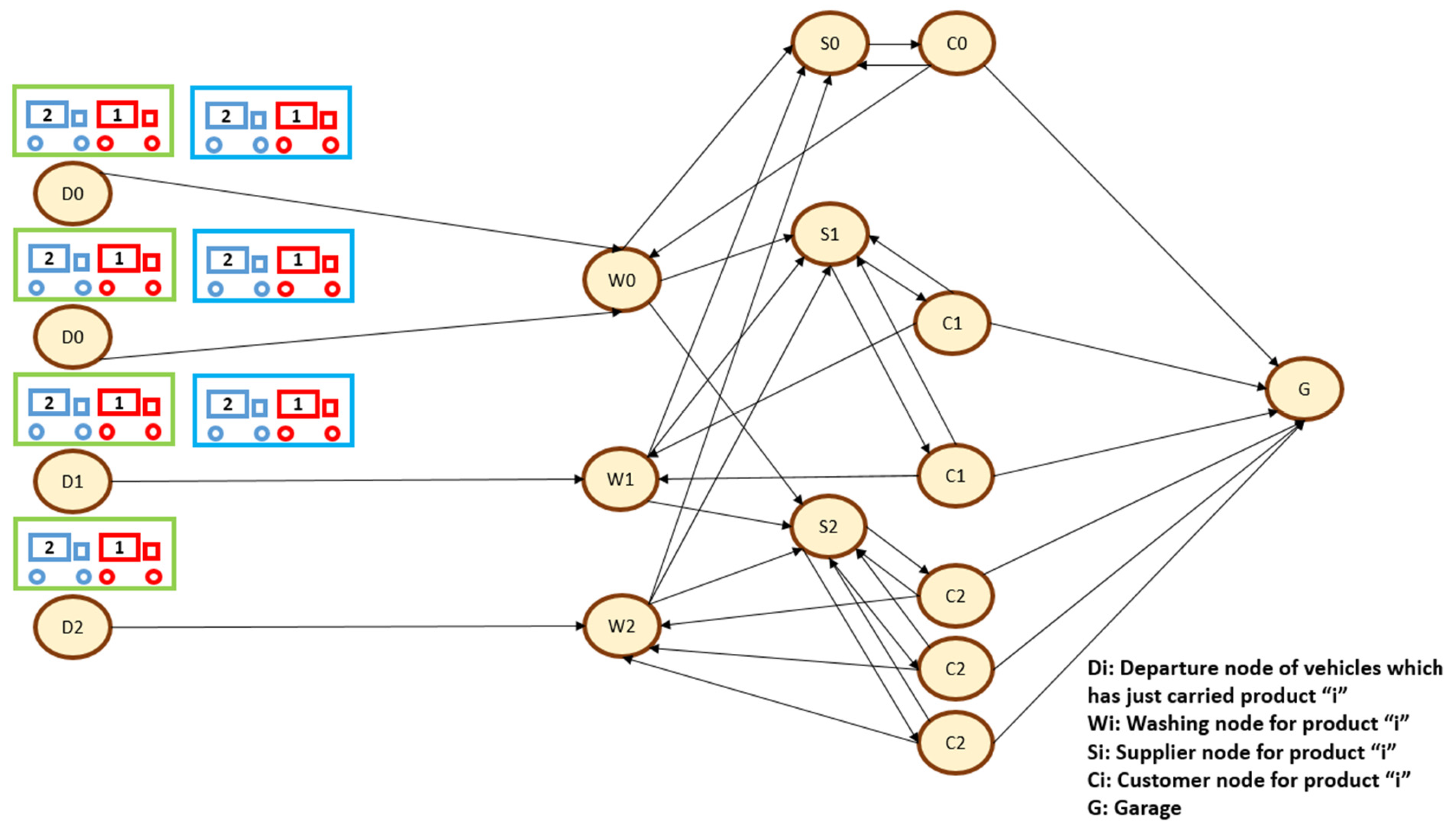
Before presenting our approach to heuristic and exact solution methods, a small-scale network structure is illustrated in Figure 2. As shown in the network representation figure, the system consists of multiple departure nodes, washing nodes, customer nodes, supply nodes, and vehicles that are capable of traversing the connecting arcs. In real-world operations, suppliers often require that logistics companies should refrain themselves from using trucks that have previously transported another product type even if that product type is similar to the suppliers’ product type by necessitating the inclusion of washing processes during transportation.

Additionally, in Figure 2, the green box represents the first type of trailer, while the blue box denotes the second type of trailer. The blue vehicle indicates the number of owned vehicles at a departure point, whereas the red vehicle represents the number of rented vehicles at the same departure point. It is evident from Figure 2 that the green trailer is capable of transporting all product types, whereas the blue trailer is restricted and cannot carry the second type of product.

As depicted in Figure 2, vehicles are forced to visit washing nodes before visiting supply nodes in order to avoid contamination after their departure. If a vehicle has completed its task with the current product type after unloading and needs to transport another product type, then that vehicle should visit the supply node of the next product type. However, the vehicle is compelled to visit the relevant washing node utilizing the arc structure depicted in Figure 2 before visiting that supply node.

In summary, a relevant idle vehicle type connected to a relevant trailer type can be observed at departure nodes in Figure 2. In the study, each washing center is a collection of $W_i$ nodes for all product types because it is assumed that a washing center is capable of washing every vehicle regardless of what they have carried previously. However, multiple washing centers can exist in a network due to their different locations. For example, $W_0, { W}_1, { W}_2$ in Figure 2 constitute a washing center (meaning the network in the figure has just one washing center in total).

It is important to note that washing nodes do not operate under time window constraints, allowing a vehicle to initiate its washing process at any time upon arrival. The duration of the washing process, however, may vary depending on the washing matrix. Therefore, when a trailer that has just carried product $X$ requires washing to carry product $Y$, the absolute difference between the minimum washing time for product $X$ in the washing matrix and the washing time required for transitioning from product $X$ to product $Y$ is taken subsequently. This difference is then added to the travel time between the current washing node and the supply node of product $Y$. Thus, the washing node always has a constant washing time for product $X$ without loss of generality throughout the CG algorithm. In this study, it is important to recall that product $X$ can only be washed at $W_x$.

Figure 3 illustrates examples of the washing matrix and trailer–product matrix. Each entry in the washing matrix represents the number of time units required to enable the transition of a trailer from carrying one product type to another type. Additionally, each entry in the trailer–product matrix indicates whether a specific trailer type is capable of loading the corresponding product.

In Figure 2, it should be noted that the blue box denotes the second type of trailer, whereas the blue vehicle indicates the number of owned vehicles at the relevant departure point. Additionally, the blue trailer is restricted and cannot carry the second type of product. When considering a subproblem and its network where a blue vehicle with blue type of trailer is about to depart from the relevant departure point, the inward arcs for the second-product-type-based supply node and second-product-type-based washing nodes have been removed (as can be seen in Figure 2, second-product-type-based customer nodes can only be visited after visiting the second-product-type-based supply node; therefore, these customers cannot be visited after the removal of the inward arcs of the second-product-type-based supply node). Thus, the relevant trailer is forced to visit relevant supply nodes on the subproblem network without violating the trailer–product matrix.

4. Methodology

4.1. Construction Heuristic

For the problem described in the network representation in Figure 2, we utilize an insertion-based method inspired by Solomon [5] that incrementally adds nodes on a route in a feasible manner until all contracted customers are served. Non-contracted customers, on the other hand, are not required to be served because they do not have to be satisfied by definition. Therefore, excluding them can reduce the heuristic’s execution time to find feasible routes.

It is well established that a CG method cannot start off without the presence of initial columns. This limitation arises because CG algorithms rely on dual variables derived from the current RMP to identify promising columns from the associated subproblem as noted by Dantzig et al. [6]. Consequently, a computationally efficient construction heuristic proposed by Solomon [5] was employed to generate the first columns required to initiate the CG process.

In the construction heuristic method, each vehicle is assigned to a route, ensuring that all vehicles depart from a designated departure node and arrive at a terminal or garage node. Therefore, arcs are added from supply nodes to garage nodes, washing nodes to garage nodes, and departure nodes to garage nodes to complete routes for each vehicle rapidly. A vehicle must adhere to time window constraints, the trailer–product matrix for product transitions and the washing matrix for washing process times until it reaches the terminal/garage node during insertions of nodes on the potential route of that vehicle. In fact, Solomon insertion method [5] decides to extend routes, creating weighted averages for each feasible extension using arc cost and travel times. However, we only care about feasible extensions during the insertion. This is because the construction heuristic is just aimed at providing initial columns/routes for CG. For the extension/insertion process in the algorithm, we display how arcs are selected for the route extension (that also means node insertion because an added node should be connected to the current route with an arc) in Algorithm 1, line 9. While there is a route and intention to insert a node, all arcs that have an intersection with the last node of the route are ordered randomly. Subsequently, the first encountered arc that ensures the feasible extension is used during the for loop in line 9 of Algorithm 1. Furthermore, a list of contracted customers is maintained during the construction heuristic execution. Each time a contracted customer is visited, it is removed from the list. In summary, non-contracted customers are not visited on these routes, while contracted customers are visited exactly once.

At the conclusion of the insertion process, it is possible that not all contracted customers have been included in the routes. Consequently, the algorithm is re-executed from the beginning until all contracted customers are successfully covered. Due to the presence of multiple time windows, the insertion heuristic prioritizes selecting the closest time window for each node during the connection process. For example, while the last node on a route is about to be connected to another node during the extension/insertion, the first daily time window of another node is checked. If infeasibility happens, violating that time window, then the second daily time window is checked. This approach enhances the potential for a route to include a greater number of customer nodes. This implementation is critical because failing to select a time window efficiently would necessitate a significantly larger number of routes (also meaning a larger number of vehicles) to cover all contracted customers. Given the limited number of vehicles available, this implementation is essential. In addition, prior to connecting a node to another node on the current route, all potential arcs for the extension are randomly ordered. These arcs are then evaluated sequentially based on this order to enhance the diversification in the heuristic algorithm.

By employing Algorithm 1, the initial routes/columns generated through the heuristic method will facilitate the execution of the exact algorithm based on CG. However, during the initial solution phase, undesirable routes, such as those which have connections between supply nodes and garage nodes or between washing nodes and garage nodes, may emerge. For example, if a vehicle is loaded, then it should proceed to unload the cargo rather than traveling to a garage or terminal node. Similarly, if a vehicle has just been washed, then it should travel to load a product instead of heading to the terminal node/garage.

To prevent the mentioned infeasible routes above from being included in the solution during the CG method, prohibitive costs (Big M values) are imposed on such connections in RMP. Subsequently, arcs connecting supply nodes to garage nodes, washing nodes to garage nodes, and departure nodes to garage nodes are removed just before the CG algorithm to ensure the generation of logical and meaningful routes for the problem.

Algorithm 1: Route Based Construction Heuristic

Feasible extensions/insertions in Algorithm 1 are applied benefiting from the label updating procedure in forward labeling using Equations (12)–(17) during the label-setting algorithm below. Additionally, the list $L$ in Algorithm 1 contains all the contracted customers in the problem, and until the list becomes empty, the algorithm tries to assign routes for the vehicles. This is because each vehicle represents a route in the whole problem.

4.2. Column Generation Algorithm

According to the literature, CG methods work rather efficiently in partitioning problems such as the generalized assignment problem (Savelsbergh [29]) or the cutting stock problem (de Carvalho et al. [30]) and VRP, while an exact algorithm is aimed at reaching optimality. Particularly, in VRP, CG methods create a leap (Desrosiers et al. [31]) in large instances compared to other exact solution techniques, such as mixed-integer programming or branch and bound or branch and cut due to their extreme efficiency. That is why the recent VRP literature is revolving around branch-price-cut algorithms based on the CG method while focusing on exact solutions. The pricing part of those algorithms is aimed at generating columns using the CG method, whereas the cutting concept is opted to obtain solutions close to integer values as in our exact algorithm for the relevant FTL transportation. Branching strategies are preferred to decrease the optimality gap further. However, our algorithm does not have any branching concept due to the fact that it already finds a low optimality gap at the root node. In short, it can be expressed that our exact algorithm can be deemed to be a part of branch-price-cut algorithms.

In VRP, the CG method needs an initial column/route set to start off; hence, construction and improvement heuristics can be deployed to reach them. Subsequently, the CG method continues to iterate itself until it attains the RMP optimality, which is a lower bound for the original problem. It is well known that the label-setting algorithm, which is employed to generate columns/routes in CG methods, has a high pseudo-polynomial time complexity due to the fact that it is the multi-dimensional version of the label-correcting algorithm (Dial et al. [32]). The label-setting algorithm consistently aims to derive promising columns/routes by utilizing the dual variables identified by RMP while adhering to the resource constraints defined for the routes/columns in the given VRP (Feillet, Dominique, et al. [33]). However, construction or improvement heuristics have polynomial time complexity. In our work, the construction heuristic and CG are serially executing algorithms and the whole solution complexity equals the maximum complexity among serial algorithms according to complexity analysis. Therefore, the overall complexity becomes pseudo-polynomial. Thus, the label-setting algorithm creates a bottleneck in the whole solution process, which is why acceleration techniques are used to generate columns faster, alleviating the impact of that bottleneck. Bi-directional search (Righini and Salani [9]), heuristic column generation (Desaulniers et al. [8]), and ng-route relaxation (Baldacci et al. [10]) techniques are aimed at accelerating the generation of promising column/route whereas the subproblem selection (an extension of the heuristic column generation technique) focuses on prioritizing the relevant subproblem, which will be capable of yielding promising columns without searching all subproblems. Regarding the exact approach, these acceleration techniques give the best performance and are widely used compared to others in current VRP literature when merged with CG methods. Thus, in our work, the most promising exact algorithm based on the CG method and the most promising acceleration techniques or concepts regarding that method in VRP literature are involved after an efficient route-based Solomon insertion method [5] has been employed. Furthermore, it must be noted that CG method and its acceleration techniques are inherently problem-dependent. Hence, this situation forces one to modify them while having a unique problem concept as we did in our work.

If all route variables were already available, the optimization of the model (1)–(8) would yield the optimal integer solution. However, the number of route variables is exceedingly large. Consequently, the optimization of the RMP is employed as an important step to compute a suitable lower bound for the original problem (1)–(8) by relaxing integer constraints. This process utilizes subproblems to identify and extract promising columns/routes so as to add them to the RMP structure. RMP is critical because of the fact that its optimal value results in a lower bound, and an upper bound can be acquired using columns generated so far.

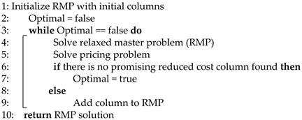
The fundamental procedure of the CG algorithm, inspired by the Dantzig–Wolfe decomposition method [6], is presented in Algorithm 2 for further examination.

Algorithm 2: Basic Column Generation

In this study, the pricing problem always needs to be solved for the given subproblem. According to the CG model (1)–(8), the total number of subproblems is $\sum _{o\in O}\sum _{i\in I_o}\sum _{j\in J}1$. Each subproblem is based on a given trailer $o\in O$ and a given departure node $i\in I_o$ for that trailer and a given vehicle type $j\in J$ connected with that trailer. Moreover, each subproblem has its own network where a relevant vehicle type connected to a relevant trailer can travel, departing from the relevant departure point. For a given subproblem network under a certain $o\in O,$ $i\in I_o$, $j\in J$, a pricing problem can be defined as follows:

$$\underset{k\in P}{\min } {\overline{c}}_{oijk}$$

The equation above is subject to the following:

Time windows constraints are respected;

Customer points should be visited at most once.

In the pricing problem above, $P$ is the subset of all routes that can exist in the given subproblem, visiting each customer node at most once as well as not violating time window structures.

$$\begin{array}{cc}\hfill {\overline{c}}_{oijk}=c_{oijk} -& {\displaystyle \sum _{q\in C}}{a}_{oijkq}\ast {\alpha }_q-{\displaystyle \sum _{q^{\prime }\in C^{\prime }}}{a}_{oijk{q}^{\prime }}\ast {\alpha }_{q^{\prime }}- {\displaystyle \sum _{U\in P\left(C\right)}}{\displaystyle \sum _{\left(m,n\right) \in A^{-}\left(U\right)}}{b}_{oijkmn}\ast {\lambda }_U\hfill \\ & - {\displaystyle \sum _{\left(m^{\prime },n^{\prime }\right) \in A^{\ast }\left(CW\right)}}{\displaystyle \sum _{\left(m,n\right) \in A^{\ast }\left(m^{\prime },n^{\prime }\right)}}{b}_{oijkmn}\ast {p1}_{m^{\prime }{n}^{\prime }}\hfill \\ & - {\displaystyle \sum _{\left(m^{\prime },n^{\prime }\right) \in A^{\ast }\left(SC\right)}}{\displaystyle \sum _{\left(m,n\right) \in A^{\ast }\left(m^{\prime },n^{\prime }\right)}}{b}_{oijkmn}\ast {p2}_{m^{\prime }{n}^{\prime }}-\beta \hfill \end{array}$$

(9)

In Equation (9), $c_{oijk}$ is the cost of the route, whereas ${\alpha }_q$, ${\alpha }_{q^{\prime }}$, ${\lambda }_U$, ${p1}_{m^{\prime }{n}^{\prime }}$, ${p2}_{m^{\prime }{n}^{\prime }}$ are the dual variables of (2), (3), (5), (6), and (7), respectively. $\beta$ is the dual variable that belongs to (4), corresponding to the current subproblem. Finally, ${\overline{c}}_{oijk}$ is the reduced cost, which belongs to the route.

4.2.1. Label-Setting Algorithm

In our study, the label-setting algorithm is aimed at extracting promising routes/columns from the pricing problem. This algorithm needs to be applied to every subproblem that we have in the CG model (1)–(8). In total, there are $\sum _{o\in O}\sum _{i\in I_o}\sum _{j\in J}1$ subproblems, each of which is based on a given trailer $o\in O$, a given departure node $i\in I_o$ for that trailer, and a given vehicle type $j\in J$ connected with that trailer. In fact, each subproblem has its own network in itself, and vehicles that can travel that network have a limit of $H_{oij }$ in (4). Therefore, the networks of all subproblems are being analyzed using the label-setting algorithm to identify promising columns/routes that have the potential to enhance the RMP. If no subproblem yields a promising column, it indicates that the optimal solution for the RMP has already been attained. Consequently, a lower bound for the CG model (1)–(8) has been established.

Michelini, Stefano, Yasemin Arda, and Hande Küçükaydin [34] addressed the VRP with time windows and variable departure times using branch price algorithms. Given that the reduction in redundant waiting times at visited nodes on routes is also a focus of our study, we adapted and applied a modified version of their approach. Furthermore, we were inspired by the work of Feillet; Dominique et al. [33]; and Righini, Giovanni, and Matteo Salani [9,35], who developed effective labeling procedures that are known as forward and backward labeling for solving elementary shortest-path problems with resource constraints. These adaptations enabled us to incorporate a tailored version of their methodologies into our problem.

Table 2. Notation of label-setting algorithm.

Sets
$N$	set of whole nodes
Variables
$v_i$,$v_i^b$	representation of ith vertex/node during forward labeling and backward labeling, respectively
$PF=(\dots ,\dots ,\dots ,v_i)$	forward path for $v_i$ during forward labeling while using forward arcs
$PB=(\dots ,\dots ,\dots ,v_i^b)$	backward path for ${v_i}^b$ during backward labeling while using reverse arcs
${\theta }_k$, ${{\theta }_k}^b$	cumulative time amount until $v_k$ and its backward labeling version until ${v_k}^b$ in the forward path and backward path, respectively
${\mu }_i$	earliest starting time at $v_i$ while having $PF=(\dots ,\dots ,\dots ,v_i)$
${{\mu }_i}^b$	backward labeling version of ${\mu }_i$ at ${v_i}^b$ while having $PB=(\dots ,\dots ,\dots ,v_i^b)$
${\left(E_i^k\right)}_{k\in N}$	indicate whether $PF=(\dots ,\dots ,\dots ,v_i)$ has visited $v_k$ or not so far
${\left(E_i^{k,b}\right)}_{k\in N}$	backward labeling version of ${\left(E_i^k\right)}_{k\in N}$ at ${v_i}^b$ while having $PB=(\dots ,\dots ,\dots ,v_i^b)$
${\zeta }_i$	minimum duration for starting at $v_i$ while having $PF=(\dots ,\dots ,\dots ,v_i)$
${{\zeta }_i}^b$	backward labeling version of ${\zeta }_i$ at ${v_i}^b$ while having $PB=(\dots ,\dots ,\dots ,v_i^b)$
$c_i$,${c_i}^b$	reduced cost value of $PF=(\dots ,\dots ,\dots ,v_i)$ and $PB=(\dots ,\dots ,\dots ,v_i^b)$, respectively
$L_i(\dots )$, ${L_i}^b(\dots )$	forward and backward label, respectively
Parameters
$[a_i,b_i]$	time windows boundaries of $v_i$ during forward labeling
$\left[a_i^b,b_i^b\right]$	time windows boundaries of ${v_i}^b$ during backward labeling

summarizes the notation for the label-setting algorithm.

Now, consider a forward path such as $PF=(v_0,v_1\dots ,v_i)$, where $v_0$ is one of the all departure nodes (departure node of the network in the current subproblem), and all nodes on that path have been visited within one of their multiple time windows, that is, $[a_i,b_i]$ for each node $v_i$. Because vehicles can leave the departure node later, let ${\nu }_i$ be the latest feasible start time from the departure node. The latest feasible start time can be written as follows:

$${\nu }_i=\underset{1\le k\le i}{\min }\left\{b_k-{\theta }_k\right\},$$

(10)

where ${\theta }_k$ is the cumulative time and always updated with ${\theta }_k={\theta }_{k-1}+{\overline{t}}_{k-1,k},$ while ${\overline{t}}_{k-1,k}=s_{k-1}+t_{k-1,k}$. Arc travel times from $v_{k-1}$ to $v_k$ are depicted as $t_{k-1,k}$, whereas $s_{k-1}$ is the process time at $v_{k-1}$. Additionally, the earliest feasible start time at node $v_i$ can be calculated as ${\mu }_i=\max \left\{a_i,{\mu }_{i-1}+{\overline{t}}_{i-1,i} \right\}$. When the forward path $PF=(v_0,v_1\dots ,v_i)$ is in existence, the minimum duration for starting at $v_i$, which is defined as ${\zeta }_i$, takes place while the vehicle employs the latest feasible start time from the departure node, which is ${\nu }_0$.

Due to the triangle inequality structure, the optimal path should be an elementary path in terms of customer points/nodes that means at the optimality an optimal route cannot visit a customer node multiple times. So, the label $\left(E_i^k\right)$ is employed for $\forall k\in N$, where $N$ is the set of whole nodes in the problem. If the partial path $PF=\left(v_0,v_1\dots ,v_i\right)$ has visited customer node $k$, then $\left(E_i^k\right)$ becomes 1 and 0 otherwise. However, in this study, there also washing and supply points/nodes instead of pure customer points/nodes. Therefore, if a node, for example, is a washing or supply node, and it has been already visited by the partial path, then $\left(E_i^k\right)$ may remain as 0 due to the fact that non-customer nodes do not need to be visited at most once in the CG model.

In short, $PF=(v_0,v_1\dots ,v_i)$ also can be expressed as ${L_i(\nu }_i, {\mu }_i,{\zeta }_i,{\left(E_i^k\right)}_{k\in N}, c_i,{\theta }_i)$, where $c_i$ is the reduced cost of the partial forward path. In order to calculate the reduced cost over a partial path, original arc costs and dual variables coming from RMP must be merged together. Therefore,

$$\begin{array}{cc}\hfill {\overline{c}}_{ij}=c_{ij}-{\alpha }_i& - {\displaystyle \sum _{U \in P\left(C\right)| \left(i,j\right)\in A^{-}(U)}}{\lambda }_U-{\displaystyle \sum _{\left(i^{\prime },j^{\prime }\right)\in A^{\ast }\left(CW\right)| \left(i,j\right)\in A^{\ast }\left(i^{\prime },j^{\prime }\right)}}{p1}_{i^{\prime }{j}^{\prime }}\hfill \\ & -{\displaystyle \sum _{\left(i^{\prime },j^{\prime }\right)\in A^{\ast }\left(SC\right)| \left(i,j\right)\in A^{\ast }\left(i^{\prime },j^{\prime }\right)}}{p2}_{i^{\prime }{j}^{\prime }} , \forall (i,j)\in \mathcal{A}\hfill \end{array}$$

(11)

where ${\alpha }_i$ is the dual variable for contracted or non-contracted customer visiting constraints coming from (2) and (3), ${\lambda }_U$ is the dual variable for k-path (k = 2) inequalities (5), ${p1}_{i^{\prime }{j}^{\prime }}$ and ${p2}_{i^{\prime }{j}^{\prime }}$ are dual variables of the relevant arc flow constraints (6) and (7), respectively, $c_{ij}$ is the cost which has been found after Floyd–Warshall algorithm with the addition of extra costs such as washing costs, and 𝒜 is the set of all arcs that can exist in the current subproblem. Therefore, the reduced cost of a partial forward path called $PF=(v_0,v_1\dots ,v_i)$ can be written as $c_i=\sum _{(k,l)\in PF}{\overline{c}}_{k,l}-\beta$. Here, $\beta$ is the constant dual variable corresponding to $\sum _{k\in K}{\theta }_{oijk}\le H_{oij }$ for a given $o\in O, i\in I_o , j\in J$ originating in constraint (4). Recall that each subproblem in our study corresponds to a given $o\in O, i\in I_o , j\in J$, and the network belonging to that subproblem is being taken into account to generate promising routes.

During the extension of label to node $j$, ${L_j(\nu }_j,{\mu }_j,{\zeta }_j,{\left(E_j^k\right)}_{k\in N},c_j,{\theta }_j)$ is obtained using the following label-updating procedure:

$$c_j=c_i+{\overline{c}}_{ij}$$

(12)

$${\zeta }_j=\max \left\{{\zeta }_i+{\overline{t}}_{i,j} ,{\mu }_j-{\nu }_j\right\}$$

(13)

$${\mu }_j=\max \left\{a_i,{\mu }_i+{\overline{t}}_{i,j}\right\}$$

(14)

$${\nu }_j=\min \left\{{\nu }_i,b_j-{\theta }_j\right\}$$

(15)

$${\theta }_j={\theta }_i+{\overline{t}}_{i,j}$$

(16)

$$\left(E_j^k\right)=\left\{\begin{array}{c}\left(E_i^k\right)+1 \\ \left(E_i^k\right)\end{array}\right.\begin{array}{c} if k=j and j \in \left(C \cup C^{\prime }\right)\\ if k\ne j or j \notin \left(C \cup C^{\prime }\right)\end{array}$$

(17)

When $\left(E_j^k\right)>1$ for a customer node $k$, then ${L_j(\nu }_j, {\mu }_j,{\zeta }_j,{\left(E_j^k\right)}_{k\in N}, c_j,{\theta }_j)$ is eliminated. For washing and supply nodes, $\left(E_j^k\right)$ always remains 0 due to the fact that those nodes can always be visited more than once, as opposed to customer nodes. However, each time a label $L_i$ is extended to create a new label $L_j$, the elementarity resource $E_j^k$ is set to zero for $k$∉$M_j$, where $M_j$ is the predetermined ng-set for node $j$. In forward labeling, ng-sets are constructed based on supply nodes because a customer node can only be reached from supply nodes, but in the backward labeling, those sets are constituted based on supply and washing nodes because, using a reverse arc, one can travel from supply or washing nodes to customer nodes (see Figure 2). All those sets are relaxation for the elementarity of customer points; thus, the lower bound may become slightly lower, but an increase in the CG algorithm’s convergence rate is established. Furthermore, if ${\mu }_j>b_j$, then ${L_j(\nu }_j, {\mu }_j,{\zeta }_j,{\left(E_j^k\right)}_{k\in N}, c_j,{\theta }_j)$ is eliminated again. Additionally, the forward label is initialized as ${L_o(\nu }_0=\infty , {\mu }_0=0, {\zeta }_0=0,{ \left(E_0^k\right)}_{k\in N}=0, c_0=0, {\theta }_0=0)$ for the relevant departure node at the beginning. It must also be noted that forward extension from $v_i$ is happening for each time window of $v_j$ due to multiple time windows of nodes in our study; therefore, this situation may yield multiple forward labels by its nature.

The similar forward label procedure above can also be applied to the backward path, such as $PB=(v_0^b,v_1^b\dots ,v_i^b)$, due to symmetry, where $v_0^b$ is the garage node. Also, using a sufficiently large enough positive constant M, the time window $[a_i,b_i]$ for each node $v_i$ becomes $\left[a_i^b,b_i^b\right]=[{M-b}_i-s_i ,{M-a}_i-s_i]$ during backward labeling. For example, $M$ can be taken as $\underset{q}{\max }\underset{i\in (C\cup C^{\prime })}{\max }(b_{iq}+s_i+t_{ig})$, where $t_{ig}$ is the travel time from node $i$ to garage node $g$ (which is $v_0^b$ at the same time), $q$ is the time window index (recall that customer and supply points’/nodes’ multiple time windows are on daily basis), and $b_{iq}$ is the upper bound of $q^{th}$ time windows for a given node $i$. It is important to reiterate that arcs can be directed exclusively to the garage node from only customer nodes since connections from other nodes to the garage node are not meaningful, as has been previously stated. Accordingly, ${{\nu }_i}^b=\underset{1\le k\le i}{\min }\{{b_k}^b-{{\theta }_k}^b\}$, where ${\theta }_k^b={\theta }_{k-1}^b+s_{k-1}+t_{k,k-1}$. In short, $PB=(v_0^b,v_1^b\dots ,v_i^b)$ can be expressed as ${L_i}^b(v_i^b, {{\mu }_i}^b,{{\zeta }_i}^b,{\left(E_i^{k,b}\right)}_{k\in N}, {c_i}^b,{{\theta }_i}^b)$, where ${c_i}^b$ is the reduced cost of the partial backward path. During the extension of label to node $j$ using the reverse arc $(i,j)$, ${L_j}^b(v_j^b, {{\mu }_j}^b,{{\zeta }_j}^b,{\left(E_j^{k,b}\right)}_{k\in N}, {c_j}^b,{{\theta }_j}^b)$ is obtained using the following label-updating procedure:

$${c_j}^b={c_i}^b+{\overline{c}}_{ji}$$

(18)

$${{\zeta }_j}^b=\max \left\{{{\zeta }_i}^b+s_i+t_{j,i} ,{{\mu }_i}^b-v_i^b\right\}$$

(19)

$${{\mu }_j}^b=\max \left\{{a_j}^b,{{\mu }_i}^b+s_i+t_{j,i}\right\}$$

(20)

$$v_j^b=\min \left\{v_i^b,{b_j}^b-{{\theta }_j}^b\right\}$$

(21)

$${{\theta }_j}^b={{\theta }_i}^b+s_i+t_{j,i}$$

(22)

$$\left(E_j^{k,b}\right)=\left\{\begin{array}{c}\left(E_i^{k,b}\right)+1 \\ \left(E_i^{k,b}\right)\end{array}\right.\begin{array}{c} if k=j and j \in \left(C \cup C^{\prime }\right)\\ if k\ne j or j \notin \left(C \cup C^{\prime }\right)\end{array}$$

(23)

In forward labeling, ng-sets are generated based on supply nodes since customer nodes can only be reached from supply nodes. Conversely, in backward labeling, these sets are constructed based on both supply and washing nodes since reverse arcs can enable travel from supply or washing nodes to customer nodes. Additionally, the initialization of backward labels is analogous to that of forward labels, owing to the symmetry in the problem structure.

Concatenation of backward and forward paths is crucial because of the fact that, for an efficient CG, the first negative reduced cost path is employed. But label dominance is required to avoid tremendous amount of labels. Otherwise, their concatenation would be so hard and time consuming. Therefore, while there are two forward labels called $L_i^1({{\nu }_i}^1, {{\mu }_i}^1,{{\zeta }_i}^1,{\left(E_i^{k,1}\right)}_{k\in N}, {c_i}^1,{{\theta }_i}^1)$ and $L_i^2({{\nu }_i}^2, {{\mu }_i}^2,{{\zeta }_i}^2,{\left(E_i^{k,2}\right)}_{k\in N}, {c_i}^2, {{\theta }_i}^2)$, the following dominance rules (24)–(29) make $L_i^1({{\nu }_i}^1, {{\mu }_i}^1,{{\zeta }_i}^1,{\left(E_i^{k,1}\right)}_{k\in N}, {c_i}^1,{{\theta }_i}^1)$ more dominant compared to $L_i^2({{\nu }_i}^2, {{\mu }_i}^2,{{\zeta }_i}^2,{\left(E_i^{k,2}\right)}_{k\in N}, {c_i}^2,{{\theta }_i}^2)$ regarding the forward labeling:

$${{\nu }_i}^1\ge {{\nu }_i}^2$$

(24)

$${{\mu }_i}^1\le {{\mu }_i}^2$$

(25)

$${{\zeta }_i}^1\le {{\zeta }_i}^2$$

(26)

$${c_i}^1\le {c_i}^2$$

(27)

$${{\theta }_i}^1\le {{\theta }_i}^2$$

(28)

$$E_i^{k,1}\le E_j^{k,2}, \forall k\in N$$

(29)

Thus, whenever $L_i^1$ and $L_i^2$ are extended to same node $j$ for a specific time window of that node using extension Equations (12)–(17), then ${{\nu }_j}^1\ge {{\nu }_j}^2$, ${{\mu }_j}^1\le {{\mu }_j}^2$, ${{\zeta }_j}^1\le {{\zeta }_j}^2$, ${c_j}^1\le {c_j}^2$, ${{\theta }_j}^1\le {{\theta }_j}^2$, $E_J^{k,1}\le E_j^{k,2}$ for all $k\in N$ are obtained regarding $L_j^1$ and $L_j^2$. The same dominance rules are again applied during backward labeling because of the symmetric concept.

Whereas forward labels are derived, according to Michelini et al. [34], ${\zeta }_i$ becomes a critical resource and forward label $L_i$ can be extended to node $j$, having a new forward label $L_j$ when ${\zeta }_j\le M/2$. The same things are again applied to backward labeling smoothly.

Label concatenation is obligatory to create new promising routes for the CG method. Therefore, the connection of forward label ${L_i(\nu }_i, {\mu }_i,{\zeta }_i,{\left(E_i^k\right)}_{k\in N}, c_i,{\theta }_i)$ and backward label ${L_i}^b(v_i^b, {{\mu }_i}^b,{{\zeta }_i}^b,{\left(E_i^{k,b}\right)}_{k\in N}, {c_i}^b,{{\theta }_i}^b)$, which correspond to the same node, can occur under the following conditions:

$$c_i+{c_i}^b<0$$

(30)

$${\mu }_i+s_i \le M-{{\mu }_i}^b$$

(31)

$$E_i^k+E_i^{k,b}\le 1, \forall k\in N \backslash \left\{v_i\right\}\cap \left(C \cup C^{\prime }\right)$$

(32)

Thus, after suitable concatenation, the column is generated, and it is added to the RMP.

4.2.2. Acceleration Techniques

In spite of the fact that the VRP literature heavily focuses on CG methods to achieve exactness in large-scale instances, acceleration techniques for those methods also draw attention considerably. For instance, in the label-setting algorithm, enormous numbers of labels are typically generated and management of them imposes a significant computational burden. Additionally, when numerous subproblems are present, their prioritization becomes crucial since searching through all potential columns within a given subproblem and identification of no promising candidates would be highly time-consuming for the solution process.

During CG methods in VRP, the label-setting algorithm must perform to feed the RMP with pseudo-polynomial complexity for each identified promising column. Therefore, a substantial acceleration for a CG implies a significant reduction in overall complexity. Thus, we incorporated four widely used acceleration techniques to enhance the convergence rate of the RMP in our study.

Heuristic Column Generator

In linear programming, the reduced cost provides a mechanism to improve the objective function, and the best reduced cost is typically prioritized to achieve optimal improvement. However, in the label-setting algorithm, identification of the column with the best reduced cost based on the dual variables of the RMP can be computationally intensive due to the fact that this circumstance requires the investigation of huge number of labels (Desaulniers et al. [8]). This is because, when an enormous number of labels exists, computationally management of those during the search for the column/route with the best reduced cost becomes exhaustive.

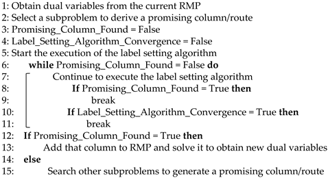
In order to save computational time, we adopted a heuristic approach by selecting the first encountered column/route with a promising reduced cost within the network of a subproblem rather than exhaustively searching for the best one. If no promising column is identified in a subproblem, other subproblems are sequentially considered. If none of the subproblems yield a promising column, it indicates that the RMP has already reached its optimal solution. The effectiveness of this approach was demonstrated by Desaulniers et al. [8] allowing the rapid identification of a promising column. The identified column is then incorporated into the RMP to generate new dual variables ensuring the continuation of the CG process. The pseudo-code of that method can also be examined in Algorithm 3 below.

Algorithm 3: Heuristic Column Generation

Subproblem Selection

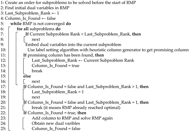
Because of the fact that our problem has high number of subproblems, which is $\sum _{o\in O}\sum _{i\in I_o}\sum _{j\in J}1$, a strategy needs to be developed to effectively make a decision on subproblem choice. Typically, it is possible to evaluate all subproblems sequentially in a predetermined order until a promising column is identified. However, this approach can significantly increase the time required to find such a column. For example, after a certain number of iterations in the RMP, some subproblems may lose their effectiveness in generating columns that can improve the RMP. Thus, solving these subproblems would result in wasted computational time. In order to address this issue, subproblem selection prioritizes the last subproblem that most recently contributed a promising column to the RMP rather than checking all subproblems sequentially.

It is important to note that subproblem selection is an extension of the heuristic column generation method (Desaulniers et al. [8]). This is because, in cases where there is only a single subproblem in the overall problem, heuristic column generation focuses on identifying the first promising column. However, subproblem selection aims to identify the first promising column across multiple subproblems. In short, subproblem selection is capable of reinforcing the heuristic column generation method and enables it to perform across multiple subproblems. The process can also be seen in Algorithm 4 as pseudo-code.

Algorithm 4: Subproblem Selection

NG-Route Relaxation

Baldacci, Roberto, Aristide Mingozzi, and Roberto Roberti [10] introduced the ng-route relaxation technique for VRP(s) with time windows. While elementary paths (visiting customer nodes/points at most once) are required in the label-setting algorithm to ensure the elementary structure of optimal paths, their approach incorporates non-elementary paths (visiting customer nodes/points multiple times) to expedite the convergence of the RMP. This relaxation substantially accelerates convergence, albeit at the cost of loosening the RMP’s lower bound. However, their study demonstrates that the loosening effect is not significant. Thus, their works can provide the addition of promising columns/routes more frequently, decreasing the convergence time of the RMP. In their method, the ng-set is defined for each node with its predetermined size, and its elements comprise neighboring nodes. Nodes within the ng-set are restricted to a single visit, whereas other nodes may be visited multiple times during the label-setting process.

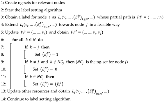
Inspired by this relaxation technique, we also allow promising routes to include non-elementary paths to a limited extent, leveraging the ng-route concept. Unlike VRP(s) that consist solely of customer nodes, our problem includes additional node types, such as washing and supply nodes in addition to departure and garage nodes. Consequently, in forward paths during forward labeling, ng-sets are created based on supply nodes since customer nodes can only be reached from supply nodes using forward arcs. Conversely, in backward paths during backward labeling, ng-sets are constructed based on supply and washing nodes since reverse arcs enable traversal from supply or washing nodes to customer nodes. Thus, all ng-sets include customer points in themselves. Algorithm 5 presents the pseudo-code of that technique as follows:

Algorithm 5: NG-Route Relaxation

Bi-Directional Search

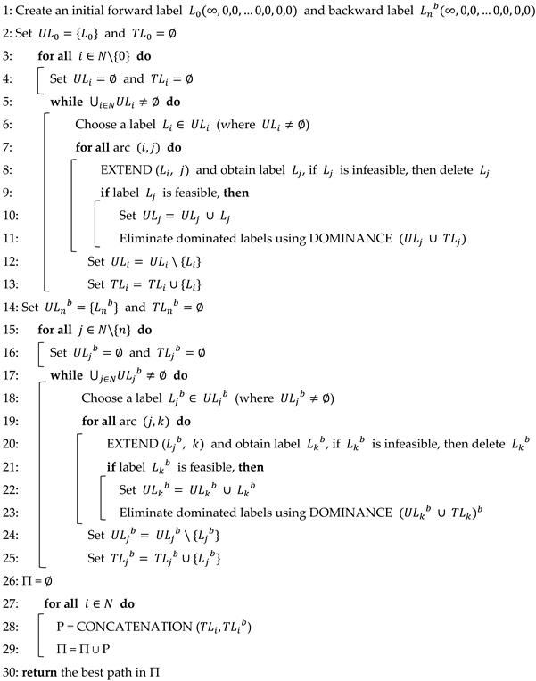
In our study, we employ both forward and backward labeling to implement a bi-directional search strategy, as proposed by Righini and Salani [9]. During forward labeling, feasible forward paths are identified using extension rules (12)–(17) while progressing towards the terminal/garage node. Conversely, backward labeling aims to identify feasible backward paths using extension rules (18)–(23) and to move towards the departure node of the current network as defined by the relevant subproblem. Righini and Salani [9] demonstrated that bi-directional search significantly outperforms mono-directional search in terms of computational efficiency. This is because they create routes using both the starting node (departure node) and terminal node (garage node), employing forward and backward labeling procedures simultaneously. In fact, the bi-directional search embraces two-dimensional perspectives during the creation of routes instead of a one-dimensional perspective like the mono-directional search. Consequently, concatenation rules are employed to combine forward and backward paths, generating promising columns/routes for the RMP.

Undoubtedly, the concatenation of forward and backward paths identified through the label-setting algorithm in the bi-directional search should encompass all paths that could be generated by the mono-directional search. To enhance efficiency, Righini and Salani [9] proposed bounding rules for forward and backward paths, which serve to restrict the further extension of these paths. In our study, we employed a resource-based bounding procedure and designated ${\zeta }_i$ to become a critical resource of paths, as was also carried out by Michelini et al. [34]. Thus, our forward paths and backward paths in the study were bounded by ${\zeta }_j\le M/2$, guaranteeing all paths which the mono-directional search would also involve. The algorithm of the bi-directional search can be examined in Algorithm 6. In this algorithm, it is assumed that the current subproblem has its network, whose departure node is the 0th node and terminal/garage node is the nth node in the whole node set that is $N$.

In Algorithm 6, ${UL}_i$ and ${TL}_i$ imply untreated labels and treated labels in the forward labeling, respectively, while ${{UL}_j}^b$ and ${{TL}_j}^b$ indicate untreated and treated labels in the backward labeling. $L_i$ means the forward label regarding the node $i$, and ${L_j}^b$ is the backward label for node $j$. EXTEND ($L_i$, $j)$ implies the forward extension of label $L_i$ along the arc $(i,j)$ to yield label $L_j$ using Equations (12)–(17), whereas EXTEND (${L_j}^b$, $k)$ is the backward version of extension using Equations (18)–(23). DOMINANCE $( )$ enables the bi-directional algorithm to be relieved of many labels using the dominance rules and inequalities (24)–(29). Moreover, CONCATENATION $( )$ can be examined in Algorithm 7 based on Algorithm 6 with the inclusion of inequalities (30)–(32).

Algorithm 6: Bi-directional Search

Algorithm 7: CONCATENATION $({TL}_i, {{TL}_i}^b$)

It must be emphasized that we do not strive for finding the best path, as shown in line 30 of Algorithm 6. In fact, we employ the bi-directional search during the label-setting algorithm instead of the mono-directional one without any effort to find the best promising column/route due to the usage of the heuristic column generation method at the same time.

5. Computational Study

5.1. Details of Experiments

Due to the absence of instances related to our problem concept in VRP literature, we generated instance sets artificially. Nevertheless, the operations of a prominent local logistics company in Turkey, which has been in the business of large-scale liquid transportation with 600 vehicles, were considered, and their processes were examined. Consequently, ranges were established for arc costs, travel times, process times, washing costs and profits associated with non-contracted customers. Random numbers were generated within these ranges using a uniform distribution.

In order to ensure the triangle inequality (as in real life cases) among arc costs and travel times within the network, the Floyd–Warshall all-pairs shortest-path algorithm (Floyd, Robert W [36]) was applied. Following this algorithm, additional costs related to washing operations or loaded positions and extra profits associated with serving the non-contracted customers were incorporated into the arc costs, which had been derived from the Floyd–Warshall [36] algorithm. Furthermore, each type of trailer was designed to accommodate at least 50% of the product types based on the trailer–product matrix, while each product type could be transported by at least one trailer type, mirroring real-life scenarios. The washing matrix was also artificially generated to reflect real-world operations closely.

The instances used in this study consist of 80% contracted customers and 20% non-contracted customers. The total number of customer points/nodes considered across different instances is {30, 60, 120}. At departure nodes, the proportion of owned to rented vehicle types varies between 65–35% and 50–50%. This circumstance happened because whenever a trailer was associated with a product type, two owned vehicles and one rented vehicle, one owned vehicle and one rented vehicle, or three owned and two rented vehicles connected to that trailer were assigned to the corresponding departure node, which contained vehicles that had previously transported that product type. Additionally, due to the presence of multiple departure nodes, the total number of departure nodes across instances is {20, 30, 40}.

This study incorporates multiple daily time windows for customers and suppliers whose number of time windows is 2, 3, or 4 during instances. For washing operations, the number of washing centers in the network was set to 3, 5, or 7 per instance. It is important to note that each washing center consists of a number of nodes equivalent to the total number of product types as illustrated in Figure 2. Moreover, the CG model (1)–(8) includes numerous cuts associated with constraints (6) and (7). In order to manage them, every 50 iterations (50 column generations), these cuts were progressively added one at a time.

The total number of product types and trailer types is {4, 6, 8} across all instances. Predetermined ng-sets in forward labeling were constructed based on supply nodes since customer nodes can only be reached from supply nodes. These ng-sets contain only customer nodes within the neighborhood of the relevant supply node, having sizes of {2, 4, 8} for the instances whose total number of customer is {30, 60, 120}, respectively. Similarly, in backward labeling, these ng-sets consist of customer nodes in the neighborhood of the relevant supply or washing node, having sizes of {2, 4, 8} for the instances whose total number of customers is {30, 60, 120}, respectively.

After RMP optimality had been reached, we called the objective $z^{lb}$, recalling that RMP during the CG method gives the lower bound of the model (1)–(8). Then, we found integer solutions using the columns/routes located in RMP, and an upper bound for our problem called $z^{\ast }$ was found, benefiting from those solutions. In order to find the optimality gap, we calculated $100\ast {\displaystyle \frac{z^{\ast }-z^{lb}}{z^{\ast }}}$ accordingly.

5.2. Results of Experiments

In total, 117 instances were generated, and their performance analysis was conducted. For each instance, the inputs included the number of time windows, product types, trailer types, washing centers, customer number, departure point, and idle vehicles. The computational time and optimality gap results were obtained based on the given inputs. All instances generated for the computational performance analysis can be examined in

Table 3. Results of all generated instances.

Number of Time Windows	Number of Product Types	Number of Trailer Types	Number of Washing Centers	Total Customer Number	Number of Departure Points	Time (s)	Optimality Gap (%)	Idle Vehicle Number
2	4	6	3	30	20	66	0	211
2	4	6	3	30	30	68	0.001504	285
2	4	6	3	30	40	154	0.013464	416
2	4	6	3	60	20	192	0.007409	205
2	4	6	3	60	30	304	0.006892	282
2	4	6	3	60	40	358	0.002384	336
2	4	6	3	120	20	868	0.000409	204
2	4	6	3	120	30	1056	0.001095	250
2	4	6	3	120	40	1291	0.001936	381
2	4	6	5	30	20	70	0.001042	213
2	4	6	5	30	30	150	0.00543	296
2	4	6	5	30	40	173	0.003775	406
2	4	6	5	60	20	231	0.005543	213
2	4	6	5	60	30	335	0.000714	282
2	4	6	5	60	40	432	0.005336	406
2	4	6	5	120	20	1068	0.000648	175
2	4	6	5	120	30	1085	0.001259	282
2	4	6	5	120	40	1854	0.00038	400
2	4	6	7	30	20	81	0	202
2	4	6	7	30	30	154	0	268
2	4	6	7	30	40	209	0.000136	442
2	4	6	7	60	20	261	0.003445	162
2	4	6	7	60	30	293	0.002451	245
2	4	6	7	60	40	500	0.004101	319
2	4	6	7	120	20	896	0.001153	213
2	4	6	7	120	30	1147	0.002981	278
2	4	6	7	120	40	1588	0	361
2	6	4	3	30	20	38	0.001683	110
2	6	4	3	30	30	86	0.003185	205
2	6	4	3	30	40	103	0.00774	286
2	6	4	3	60	20	150	0.001646	117
2	6	4	3	60	30	301	0.001703	185
2	6	4	3	60	40	378	0.007842	283
2	6	4	3	120	20	778	0.000172	150
2	6	4	3	120	30	1239	0.000251	184
2	6	4	3	120	40	1318	0.00192	290
2	6	4	5	30	20	77	0.012292	135
2	6	4	5	30	30	119	0.011543	216
2	6	4	5	30	40	162	0.016198	312
2	6	4	5	60	20	229	0.000325	119
2	6	4	5	60	30	393	0.001269	195
2	6	4	5	60	40	431	0.009255	212
2	6	4	5	120	20	846	0.00145	177
2	6	4	5	120	30	1434	0.002015	219
2	6	4	5	120	40	2014	0.000335	208
2	6	4	7	30	20	86	0	152
2	6	4	7	30	30	169	0.004965	216
2	6	4	7	30	40	209	0.00317	249
2	6	4	7	60	20	268	0.00387	130
2	6	4	7	60	30	489	0	197
2	6	4	7	60	40	558	0	276
2	6	4	7	120	20	1084	0.000349	155
2	6	4	7	120	30	2009	0.002035	176
2	6	4	7	120	40	1673	0.000583	272
3	4	8	3	30	20	79	0.01133	283
3	4	8	3	30	30	115	0.02052	368
3	4	8	3	30	40	209	0	486
3	4	8	3	60	20	320	0.011837	250
3	4	8	3	60	30	362	0.008242	337
3	4	8	3	60	40	723	0.007918	555
3	4	8	3	120	20	1663	0.003991	282
3	4	8	3	120	30	2183	0.002882	348
3	4	8	3	120	40	2984	0.005002	416
3	4	8	5	30	20	109	0.008376	262
3	4	8	5	30	30	165	0.003161	370
3	4	8	5	30	40	300	0.004484	516
3	4	8	5	60	20	358	0.006682	247
3	4	8	5	60	30	505	0.010832	445
3	4	8	5	60	40	649	0.004283	432
3	4	8	5	120	20	2103	0	222
3	4	8	5	120	30	2588	0.003251	424
3	4	8	5	120	40	2999	0.002644	484
3	4	8	7	30	20	149	0.00176	233
3	4	8	7	30	30	190	0.000787	438
3	4	8	7	30	40	263	0.001167	564
3	4	8	7	60	20	410	0.010249	252
3	4	8	7	60	30	642	0.004233	367
3	4	8	7	60	40	896	0.006561	446
3	4	8	7	120	20	1888	0.000835	256
3	4	8	7	120	30	2492	0.000828	324
3	4	8	7	120	40	3329	0.001285	572
3	8	4	3	30	20	79	0.003928	122
3	8	4	3	30	30	152	0.006709	222
3	8	4	3	30	40	261	0.002199	262
3	8	4	3	60	20	306	0.004119	122
3	8	4	3	60	30	336	0.007213	173
3	8	4	3	60	40	749	0.001538	260
3	8	4	3	120	20	1703	0.005609	190
3	8	4	3	120	30	2101	0.006464	214
3	8	4	3	120	40	3114	0.007332	272
3	8	4	5	30	20	173	0.00079	115
3	8	4	5	30	30	174	0.011344	219
3	8	4	5	30	40	363	0.005943	257
3	8	4	5	60	20	441	0.003685	128
3	8	4	5	60	30	594	0.007789	190
3	8	4	5	60	40	1116	0.01452	280
3	8	4	5	120	20	2322	0.006227	148
3	8	4	5	120	30	2741	0.003363	169
3	8	4	5	120	40	3472	0.005986	297
3	8	4	7	30	20	181	0	132
3	8	4	7	30	30	283	0	157
3	8	4	7	30	40	362	0.001083	304
3	8	4	7	60	20	749	0.020051	108
3	8	4	7	60	30	857	0.005443	143
3	8	4	7	60	40	1384	0.009679	252
3	8	4	7	120	20	2811	0.007037	188
3	8	4	7	120	30	3337	0.004302	213
3	8	4	7	120	40	4948	0.006645	304
4	8	8	7	30	20	421	0.011281	271
4	8	8	7	30	30	742	0.012467	400
4	8	8	7	30	40	1136	0.005035	553
4	8	8	7	60	20	1824	0.010742	292
4	8	8	7	60	30	1973	0.012757	380
4	8	8	7	60	40	3502	0.010559	502
4	8	8	7	120	20	8663	0.005802	244
4	8	8	7	120	30	10,641	0.008517	403
4	8	8	7	120	40	11,457	0.004953	486

.

5.3. Discussion of Results

It can be seen in the VRP literature that CG-based exact algorithms analyze CPU(s) mostly with one dimension, the total number of customers. This is because, for example, their networks mostly consist of just one time window for each node and one departure node. However, in our work, we have multiple time windows for each node as well as multiple departure nodes, and those structures aggravate CPU(s) as well. Therefore, investigation of CPU(s) with multi-dimensions makes sense. In our study,

Table 4. CPU(s) analysis compounded by number of total customers, product types, and trailer types.

			Customer Size	30			60			120
			Number of Trailer Types	4	6	8	4	6	8	4	6	8
Number of Product Types	4	Avg CPU(s)			125	175		323	541		1206	2470
		Min CPU(s)			66	79		192	320		868	1663
		Max CPU(s)			209	300		500	896		1854	3329
		Number of Instances			9	9		9	9		9	9
	6	Avg CPU(s)		117			355			1377
		Min CPU(s)		38			150			778
		Max CPU(s)		209			558			2014
		Number of Instances		9			9			9
	8	Avg CPU(s)		225		766	726		2433	2950		10,253
		Min CPU(s)		79		421	306		1824	1703		8663
		Max CPU(s)		363		1136	1384		3502	4948		11,457
		Number of Instances		9		3	9		3	9		3

and

Table 5. CPU(s) analysis compounded by number of total customers, washing centers, and fleet size.

			Customer Size	30			60			120
			Fleet Size	L	M	S	L	M	S	L	M	S
Number of Washing Centers	3	Avg CP(s)		159	133	67	723	412	257	2153	1788	1388
		Min CPU(s)		115	68	38	723	304	150	1291	1056	778
		Max CPU(s)		209	261	86	723	749	336	2984	3114	2101
		Number of Instances		3	5	4	1	6	5	3	4	5
	5	Avg CPU(s)		213	196	123	529	603	387	2480	2220	1738
		Min CPU(s)		165	109	70	432	335	229	1854	1085	846
		Max CPU(s)		300	363	174	649	1116	594	2999	3472	2741
		Number of Instances		3	4	5	3	3	6	3	3	6
	7	Avg CPU (s)		508	259	160	1753	828	525	6754	3469	2027
		Min CPU(s)		190	149	81	642	293	261	1588	1147	896
		Max CPU(s)		1136	421	283	3502	1824	857	11,457	8663	3337
		Number of Instances		5	5	5	4	6	5	4	6	5

present a three-dimensional perspective towards CPU(s).

In Table 4, due to the extensive number of breakdowns originating from multiple dimensions of inputs, it was not feasible to include all possible instances. We have six input parameters: number of time windows, product types, trailer types, washing centers, total customers, and departure points. Each of them takes three different values, which implies that a huge number of breakdowns is in existence. Nevertheless, gathering a sufficient amount of data for each breakdown would require a tremendous amount of computational time. Therefore, a selected subset of instances (117 instances in total) was analyzed to provide sufficient insights for the problem. Instances that were excluded are represented by blanks in the table. It is observed that the instance with 120 total customers, 8 trailer types, and 8 product types exhibits the highest average computational time. Additionally, when the number of trailer types or product types increases while the number of customers are 30, 60, or 120, the computational time tends to rise significantly. Specifically, when the total number of customers is 120 and the number of product types is fixed at 8, a substantial percentage increase in computational time can be observed, while the number of trailer types goes up from 4 to 8. That increase in CPU, which is approximately 350%, is almost the same when the total number of customers is 30 or 60 instead of 120. Similarly, when the total number of customers is 120 and the number of trailer types is fixed at 8, a marked increase in the computational time occurs, whereas the number of product types increases from 4 to 8. An approximately 450% difference in the CPU time emerges during that increase in the number of product types. The same circumstance with the same percentage increase can also be observed, while the number of total customers is 30 or 60.

In Table 5, it is evident that the highest computational times occur when there are 120 customers, 7 washing centers, and a large fleet size. A significant percentage increase in computational time is observed when the number of washing centers is going up from 3 to 7 while having 120 customers with a large fleet size. Furthermore, for 120 customers and 7 washing centers, the computational time undergoes a huge percentage increase, whereas the fleet size shifts from small to large. However, those two percentage increases are so close to each other; the first of them is approximately 313%, and the second one is almost 333%. The same observation can also be made when the total number of customers is 30 instead of 120, and a 317% increase takes place for both cases. Although, these percentage increases become different, whereas the same observation with 60 customers is in existence. It is important to note that, in Table 4, a small-sized fleet (S) comprises a maximum of 220 vehicles, whereas a medium-sized fleet (M) consists of 221 to 340 vehicles. A large-sized fleet (L) includes more than 340 vehicles but fewer than 600.

Recalling that our problem involves high-dimensional structures and each input has its own breakdowns, one can examine the CPU(s) in a multi-dimensional frame. Thus, Figure 4 enables one to investigate the two-dimensional variation of CPU(s) among instances. In Figure 4, one of those dimensions is always labeled the number of customer points, as the VRP literature is familiar with. However, in order to complete the two-dimensional frame, the other dimension is selected among fleet size, the number of time windows, departure points, the number of product types, trailer types, and washing centers. The VRP literature widely acknowledges that an increase in the number of customer nodes significantly escalates the solution time in VRP. However, as illustrated in Figure 4, other factors, such as fleet size, the number of time windows, the number of washing centers, the number of departure nodes, and the number of product and trailer types, can further exacerbate the challenges posed by a large number of customers. In short, we aim to examine how the CPU time reacts when extra complexities are added to our specified FTL network. For example, instances that have a high number of time windows and a high number of customer points increases the CPU time more exponentially than ones which have a high number of washing centers and high number of customer points. In particular, Figure 4b demonstrates that the increase in the number of time windows intensifies the solution time more substantially compared to Figure 4a–f, while the number of customers grows. This effect is evident because the divergence between lines in Figure 4b becomes more pronounced as the customer size increases. In contrast, Figure 4d reveals that an increase in the number of departure points results in an almost linear shift in solution time as opposed to others, whereas the number of customers rises due to the fact that the divergence between lines is not growing considerably. Additionally, with respect to Figure 4e,f, it can be inferred that CPU time is more sensitive in Figure 4f. This is because the divergence between lines is more apparent in Figure 4f. This situation implies that while instances with a high number of customers are observed, the CPU time tends to react more significantly with the rising number of trailer types than with the growing number of product types. Regarding Figure 4a,c, it can be deduced that the reaction of the CPU time tends to be more elevated in Figure 4a due to the divergence between lines being more obvious. This circumstance indicates that while instances with a high number of customers are observed, the CPU time tends to respond more visibly to the increase in fleet size than to the increase in washing centers.

Nevertheless, our algorithms were implemented on Visual Studio (2020), and linear programming models were solved with IBM ILOG CPLEX 12.9. (IBM 2020) using a computer with 2.4 GHz Intel i7-13700 processor and 32 GB RAM running on a Windows 11 operating system. One can also observe all detailed results regarding our instances in Table 5.

6. Conclusions

This study addresses the FTL problem, which is a critical and widely encountered operation in the logistics sector. The proposed algorithm can be applied to reach the exact solution when information related to vehicles and customers is apparent. If demands owned by the logistic firm have been categorized as contractual or non-contractual, specifying the product types and the number of time windows within which those orders can be met, then those inputs can be put into the algorithm. Furthermore, the information regarding which type of available vehicle can depart with which type of trailer from a specific location can be embedded into the inputs of the algorithm as well as the details of washing centers. Afterwards, involving relevant transportation costs, travel times, and profits originating from satisfying non-contracted customers, a logistic firm can find out the optimal total transportation cost and optimal routes for designated vehicles by arranging the departure time of those vehicles to reduce waiting times at relevant locations on their routes as well.

The performance results indicate that small optimality gaps of less than 1% can be achieved within reasonable computational times even in the large-scale instances of the logistic firm that inspired our work. Specifically, optimality can be attained within three and a half hours for instances involving up to one-hundred-and-twenty customer points, eight product and trailer types, seven washing centers, four time windows, and forty departure points. Furthermore, it can be noted that the computational time required for optimization over extended time horizons with a large number of customers tends to rise substantially. This is mainly due to the fact that the CPU time is most affected by the increase in the number of time windows as the number of customers increases, as shown in the Computational Study Section. Undoubtedly, the computational time can also be reduced significantly by employing enterprise processors or servers in chip markets.

However, one of the limitations of this study is the absence of a benchmark dataset for the relevant FTL problem concept, which necessitated the creation of artificial instances. Furthermore, the large number of breakdowns caused by the high number of parameters entails a huge consumption of time to collect a sufficient amount of data for each breakdown regarding further analysis.

Future research could explore more complex networks, diverse vehicle types, driver constraints, and dynamic optimization in FTL operations. This includes incorporating electric vehicles and drones, considering driver rest requirements, and applying stochastic and dynamic optimization techniques to address uncertainties in transportation processes. Overall, future studies should focus on evolving vehicle, driver, and network concepts in FTL transportation.

References

1. Konstantakopoulos, G.D.; Gayialis, S.P.; Kechagias, E.P. Vehicle routing problem and related algorithms for logistics distribution: A literature review and classification. Oper. Res. 2022, 22, 2033–2062. [Google Scholar]
2. Sampson, J.R. Adaptation in natural and artificial systems (John H. Holland). SIAM Rev. 1976, 18, 529. [Google Scholar] [CrossRef]
3. Dorigo, M.; Maniezzo, V.; Colorni, A. Ant system: Optimization by a colony of cooperating agents. IEEE Trans. Syst. Man Cybern. Part B (Cybern.) 1996, 26, 29–41. [Google Scholar] [CrossRef] [PubMed]
4. Glover, F. Future paths for integer programming and links to artificial intelligence. Comput. Oper. Res. 1986, 13, 533–549. [Google Scholar] [CrossRef]
5. Solomon, M.M. Algorithms for the vehicle routing and scheduling problems with time window constraints. Oper. Res. 1987, 35, 254–265. [Google Scholar] [CrossRef]
6. Dantzig, G.B.; Philip, W. Decomposition principle for linear programs. Oper. Res. 1960, 8, 101–111. [Google Scholar] [CrossRef]
7. Costa, L.; Contardo, C.; Desaulniers, G. Exact branch-price-and-cut algorithms for vehicle routing. Transp. Sci. 2019, 53, 946–985. [Google Scholar] [CrossRef]
8. Desaulniers, G.; Lessard, F.; Hadjar, A. Tabu search, partial elementarity, and generalized k-path inequalities for the vehicle routing problem with time windows. Transp. Sci. 2008, 42, 387–404. [Google Scholar] [CrossRef]
9. Righini, G.; Salani, M. Symmetry helps: Bounded bi-directional dynamic programming for the elementary shortest path problem with resource constraints. Discret. Optim. 2006, 3, 255–273. [Google Scholar] [CrossRef]
10. Baldacci, R.; Mingozzi, A.; Roberti, R. New route relaxation and pricing strategies for the vehicle routing problem. Oper. Res. 2011, 59, 1269–1283. [Google Scholar] [CrossRef]
11. Ball, M.O.; Golden, B.; Assad, A.A.; Bodin, L. Planning for truck fleet size in the presence of a common-carrier option. Decis. Sci. 1983, 14, 103–120. [Google Scholar] [CrossRef]
12. Desrosiers, J.; Laporte, G.; Sauve, M.; Soumis, F.; Taillefer, S. Vehicle routing with full loads. Comput. Oper. Res. 1988, 15, 219–226. [Google Scholar] [CrossRef]
13. Soleilhac, G.; Lehuédé, F.; Medina, J.; Péton, O. The Vehicle Routing Problem with FTL and LTL Carriers. Ph.D. Thesis, IMT Atlantique, Nantes, France, 2022. [Google Scholar]
14. Ghilas, V.; Hedtke, I.; Weise, J.; Van Woensel, T. Spot market versus full charter fleet: Decision support for full truck load tenders. EURO J. Decis. Process. 2022, 10, 100022. [Google Scholar] [CrossRef]
15. El Bouyahyiouy, K.; Bellabdaoui, A. The selective full truckload multi-depot vehicle routing problem with time windows: Formulation and a genetic algorithm. Int. J. Supply Oper. Manag. 2022, 9, 299–320. [Google Scholar]
16. Ghorpade, T.; Rangaraj, N. Order first split second heuristic for alternative routing strategy for freight railways. Transp. Policy 2022, 124, 139–148. [Google Scholar] [CrossRef]
17. Fadda, P.; Mancini, S.; Serra, P.; Fancello, G. The heterogeneous fleet vehicle routing problem with draft limits. Comput. Oper. Res. 2023, 149, 106024. [Google Scholar] [CrossRef]
18. Çabuk, S.; Erol, R. Solving Dynamic Full-Truckload Vehicle Routing Problem Using an Agent-Based Approach. Mathematics 2024, 12, 2138. [Google Scholar] [CrossRef]
19. Lu, F.; Du, Z.; Wang, Z.; Wang, L.; Wang, S. Towards enhancing the crowdsourcing door-to-door delivery: An effective model in Beijing. J. Ind. Manag. Optim. 2025, 21, 2371–2395. [Google Scholar] [CrossRef]
20. Masmoudi, M.A.; Anna Kuzmicz, K.; Pesch, E.; Demir, E.; Hosny, M. Container truck transportation routing as a mixed fleet heterogeneous dial-a-ride problem. In Proceedings of the 9th International Conference on Engineering, Project, and Production Management (EPPM2018), Cape Town, South Africa, 24–26 November 2018; Volume 312. [Google Scholar]
21. Nasr, N.; Niaki ST, A.; Hussenzadek Kashan, A.; Seifbarghy, M. An efficient solution method for an agri-fresh food supply chain: Hybridization of Lagrangian relaxation and genetic algorithm. Environ. Sci. Pollut. Res. 2021, 1–19. [Google Scholar] [CrossRef]
22. Xue, N.; Bai, R.; Qu, R.; Aickelin, U. A hybrid pricing and cutting approach for the multi-shift full truckload vehicle routing problem. Eur. J. Oper. Res. 2021, 292, 500–514. [Google Scholar] [CrossRef]
23. Baller, R.; Fontaine, P.; Minner, S.; Lai, Z. Optimizing automotive inbound logistics: A mixed-integer linear programming approach. Transp. Res. Part E Logist. Transp. Rev. 2022, 163, 102734. [Google Scholar] [CrossRef]
24. El Bouyahyiouy, K.; Bellabdaoui, A. A Genetic-Based Algorithm for Commodity Selection and Full Truckload Vehicle Routing Problem. In International Conference on Digital Technologies and Applications; Springer Nature: Cham, Switzerland, 2023; pp. 806–816. [Google Scholar]
25. Melchiori, L.; Nasini, G.; Montagna, J.M.; Corsano, G. Resources synchronization in a full truckload pickup and delivery problem: An exact approach. Comput. Oper. Res. 2023, 151, 106118. [Google Scholar] [CrossRef]
26. El Bouyahyiouy, K.; Annouch, A.; Bellabdaoui, A. An MILP-based Lexicographic Approach for Robust Selective Full Truckload Vehicle Routing Problem. Int. J. Adv. Comput. Sci. Appl. 2023, 14, 642–650. [Google Scholar] [CrossRef]
27. Kohl, N.; Desrosiers, J.; Madsen, O.B.; Solomon, M.M.; Soumis, F. 2-path cuts for the vehicle routing problem with time windows. Transp. Sci. 1999, 33, 101–116. [Google Scholar] [CrossRef]
28. Kallehauge, B.; Larsen, J.; Madsen, O.B.; Solomon, M.M. Vehicle Routing Problem with Time Windows; Springer: Greer, SC, USA, 2005. [Google Scholar]
29. Savelsbergh, M. A branch-and-price algorithm for the generalized assignment problem. Oper. Res. 1997, 45, 831–841. [Google Scholar] [CrossRef]
30. de Carvalho, J.M.V. Exact solution of cutting stock problems using column generation and branch-and-bound. Int. Trans. Oper. Res. 1998, 5, 35–44. [Google Scholar] [CrossRef]
31. Desrosiers, J.; Soumis, F.; Desrochers, M. Routing with time windows by column generation. Networks 1984, 14, 545–565. [Google Scholar] [CrossRef]
32. Dial, R.; Glover, F.; Karney, D.; Klingman, D. A computational analysis of alternative algorithms and labeling techniques for finding shortest path trees. Networks 1979, 9, 215–248. [Google Scholar] [CrossRef]
33. Feillet, D.; Dejax, P.; Gendreau, M.; Gueguen, C. An exact algorithm for the elementary shortest path problem with resource constraints: Application to some vehicle routing problems. Netw. Int. J. 2004, 44, 216–229. [Google Scholar] [CrossRef]
34. Michelini, S.; Yasemin, A.; Hande, K. Branch-and-price algorithms for a VRP with time windows and variable departure times. In Proceedings of the IFORS 2017-21st Conference of the International Federation of Operational Research Societies, Québec City, QC, Canada, 17–21 July 2017. [Google Scholar]
35. Righini, G.; Matteo, S. New dynamic programming algorithms for the resource constrained elementary shortest path problem. Netw. Int. J. 2008, 51, 155–170. [Google Scholar] [CrossRef]
36. Floyd, R.W. Algorithm 97: Shortest path. Commun. ACM 1962, 5, 345. [Google Scholar] [CrossRef]
Figure 1. Example of routes that can be traveled by vehicles connected to relevant trailers departing from relevant departure nodes.
Mathematics 13 00876 g001
Figure 2. Network representation.
Mathematics 13 00876 g002
Figure 3. Trailer–product and washing matrices.
Mathematics 13 00876 g003
Figure 4. CPU(s) analysis with the number of total customers compounded by the fleet size (a). CPU(s) analysis with the number of total customers compounded by the number of time windows (b). CPU(s) analysis with the number of total customers compounded by the number of washing centers (c). CPU(s) analysis with the number of total customers compounded by the number of departure points (d). CPU(s) analysis with the number of total customers compounded by the number of product types (e). CPU(s) analysis with the number of total customers compounded by the number of trailer types (f).
Mathematics 13 00876 g004