A Study of the Colombian Stock Market with Multivariate Functional Data Analysis (FDA)

Abstract

In this work, Functional Data Analysis (FDA) is used to detect behavioral patterns in the Bolsa de Valores de Colombia (BVC) in reaction to the global crises caused by COVID-19 and the war in Ukraine. The oil price fluctuation curve is considered a covariate. The FDA’s distinctive ability is to represent stock values as smooth curves that evolve over time and provide new insights into the dynamics of the BVC. The methodology makes use of functional multivariate techniques applied to the smoothed curves of the closing prices of the main stocks of the BVC. The results show that the correlations of the oil curve with the average market curve change from almost null or low in the global period to extremely significant in time windows immediately after the beginnings of COVID-19 and the war in Ukraine, respectively. On the other hand, the velocity curves, which are used to evaluate the stock market volatility, show a pattern of synchronization of companies in the crisis periods. Furthermore, in these crisis periods, the companies in BVC showed a high synchronization with the Brent crude oil price. In conclusion, this work shows the usefulness of the FDA as a complement to time series analysis in the study of stock markets. The results of this research could be of interest to academic researchers, financial analysts, or institutions.

1. Introduction

Since its creation in 1929, the Bolsa de Valores de Colombia (BVC) has compiled daily measurements of registered securities issuers. The evolution of these values and, as a consequence, the Colombian economy depends largely on oil exports [1]. Several articles analyze the evolution of oil prices and their impact on world economies [2,3,4].

The price of a barrel of oil, regulated by OPEC since 1973, has experienced wide fluctuations determined by conflicts and geopolitical factors. In particular, a negative bubble in oil prices occurred in 2014/2015 [5]. The factors that may influence have been analyzed in an extensive note from the World Bank Group, presented by Baffes [6] in 2015.

The availability of stock values, almost in real time, makes the use of Functional Data Analysis (FDA) techniques possible and even advisable. The FDA allows each stock market security to be represented by a curve for any given time period. The curves are obtained by applying smoothing techniques to the stock market series, for which a basis of functions is needed. FDA was introduced by Ramsay and Silverman [7,8]. They extend classical statistics to the case of functions by implementing most of the classical methods.

In recent years, the analysis of the impact of global crises on different financial markets has become a common problem [9]. Firstly, in 2020, the COVID-19 virus spread throughout the world and led all countries to develop measures to prevent viral transmission, which had a major impact on the global economy, reflected in stock market trends [10]. On the other hand, in February 2022, Russia launched a full-scale invasion of Ukraine and began occupying more of the country, starting the biggest conflict in Europe since World War II. Sanctions against the invaders by a large number of countries, led by the countries of the European Union and the United States, were not long in coming. As Russia is one of the main suppliers of oil and gas, a large part of the actions focused on restrictions on the purchase of these raw materials. The consequences in the markets of both crises were reflected in high volatility.

Not all countries suffered the consequences of these two crises in the same way. The strength of the economies and the degree of dependence on oil derivatives were two of the most important factors. In this context, we decided to study the behavior of an emerging economy, such as Colombia.

This paper is organized as follows. In Section 2, the articles related to this work are presented. In Section 3, the used data are described in the first part and the FDA methods used in the paper are presented in the second part. This part includes the description of the functional data processing, the introduction of the functional correlation measure, and the FDA methods used. These methods are the k-means clustering and the FPCA techniques. In Section 4, the previous procedures are applied to the data of the Colombian Stock Exchange. Finally, in Section 5, the main conclusions are shown.

2. Literature Review

Several authors have analyzed the advantages of FDA compared to other ways of treating data, in particular, the classical times series [11,12,13,14]. According to Allen [11], “From a statistical viewpoint, time series analysis is extremely beneficial. From a mathematical viewpoint, FDA adds a modern twist on typical analysis. While one method is not meant to replace the other, each one has advantages over the other one”. Moreover, Gertheiss et al. assert in [12]: “In contrast to simpler methods that reduce the functional observations to scalar summary values, FDA retains all important information by directly using the functional observations in the analysis”. In different situations, the elements of the study are part of a continuous dynamic process, and, in this case, FDA has the advantage of exploring the dynamic information implicit in static data. Furthermore, in these cases, the analysis of the functional curve, speed curve, and acceleration curve can provide a global view of the problem under study. An example of this can be found in [13], where FDA is used to investigate the changes in energy security from a dynamic perspective.

According to Ullah [14], “In contrast to most other methods commonly used to model trends in time series data, a key strength of the FDA approach is that it makes no parametric assumptions about age or time effects. The FDA methods for modeling and forecasting data across a range of health and demographic issues also have significant advantages for better understanding trends, risk factor relationships, and the effectiveness of preventive measures”. Another advantage is that FDA does not require the stationarity condition of the data, which are treated in their original form. In practice, FDA adapts to any type of scenario and to high-frequency data. The smoothing methods used in FDA allow good control of overparameterization and produce curves with good metric and analytical properties, usually functions of class two. The first derivatives of the obtained functions give us the curves of the rate of change in the functional data, which opens a very promising field of study in a fundamental subject such as market volatility.

The way in which the FDA is applied depends on the area in question: Medicine, Meteorology, Economics, or other fields. In each field, it is important to use an appropriate methodology for the type of data. In Pérez-Plaza et al. [15], the methods used to filter, smooth, and analyze data are appropriate for seismic data. In the field of Economics, several authors have made important contributions thanks to the perspective of the FDA. Works that analyze the stock market are special due to the nature of their data, and generally, there is no specific methodology. In this field, Aguilera [16] considers weekly observations of a random sample of banks listed on the Madrid Stock Exchange, applying the Functional Principal Component Analysis (FPCA) to model and forecast prices for Spanish banks. Ingrassia and Costanzo [17] carry out an exploratory analysis of the Italian Stock Market by using FDA, suggesting the possibility of constructing a stock index based on functional indicators. Dablemont [18] presents a functional method for clustering, modeling, and forecasting time series by using functional analysis and neural networks. This method can be applied to any type of time series but is particularly effective when observations are irregularly spaced, occur at different time points for each curve, or when only fragments of the curves are observed. Benko [19], in his doctoral thesis, demonstrates the efficiency of using the functional data approach for high volatility problems, common in financial markets. His work focuses on the study of Euribor rate curves. Moreover, in the case of the Colombian stock market, there are no references to the use of FDA. Das [20] presents a new regression approach derived from FDA to analyze the effect of global crises on stock market correlations. Das employs a wide range of global crises (from the beginning of the 19th century) that have not yet been examined in the literature in this context.

Traditionally, the volatility study has been based on statistical measures of dispersion. Low volatility is related to stable market values and reduced risk levels, while high volatility is often associated with convulsive scenery and high levels of risk. In the analysis of high-frequency financial data, as well as in stock markets, volatility will be given as a function of time. In any case, it is not a directly measurable magnitude and should be estimated from the dispersion of the values; different methods and procedures are used for this purpose. From the perspective of time series, different solutions have been proposed to estimate volatility most of them based on Autoregressive conditional Heteroscedasticity (ARCH) models or Generalized Autoregressive Conditional Heteroscedasticity (GARCH) models; the works of Andersen and Bollerslev [21], Engle [22], Engle and Gallo [23] and, more recently, Engle and Sokalska [24] and Narsoo [25] are of special interesting in this context. On the other hand, from the perspective of FDA, the estimation of volatility can be obtained from the adaptation of the autoregressive models to the functional field (see Müller [26] or Shang [27]). Different works analyze the price of crude oil and other stock market indices during periods of extreme events [28,29], although these papers employ time series procedures. In his PhD thesis [30], Wei applies FDA techniques to high-frequency intraday volatility data sets, develops methods for performing short-term dynamic forecasts in real time, and introduces a proximity measurement functional curve clustering algorithm applied to a COVID-19 functional data set.

In this work, since volatility is an indicator of the variation of the prices over time, we propose to use the first derivatives of the functions in order to explore the volatility of BVC values from the velocity curves. In any case, the point of view of volatility that we propose in this work is different from intra-daily volatility, which is usually used in stock market literature, since, in our case, it is a functional volatility at each instant of time. From a graphical perspective, the speed curves show the historical behavior of the market and from an analytical point of view, the determination of the curves allows us to make forecasts.

The general objective of this article is to introduce the methodology based on FDA for the study of a stock market with the Colombian typology, characterized by its high dependence on the price of oil and with high illiquidity sceneries. FDA’s ability to represent stock market values as smooth curves over time offers a potential solution to the challenges posed by market illiquidity. By employing smoothing techniques on the available stock market series, this study can capture underlying patterns and trends that might be overlooked by conventional methods.

In order to specify the general objective, three operational objectives are established to which we will try to respond under the framework of FDA. The first and foremost objective investigates the temporal fluctuations and patterns exhibited by the stock curves and seeks to understand the complexities that govern the dynamics of the Colombian market, particularly in the two times after the beginning of the crises caused by COVID-19, and for the war in Ukraine. Secondly, the functional correlations between the Brent crude oil prices and the BVC average curve are obtained and analyzed. Moreover, the average correlation of each company in BVC to the other curves is calculated, comparing the results of the global period with those obtained in the two time windows described. Thirdly, FPCA is used in order to detect similar behavior in the BVC companies.

3. Materials and Methods

3.1. Functional Data Processing

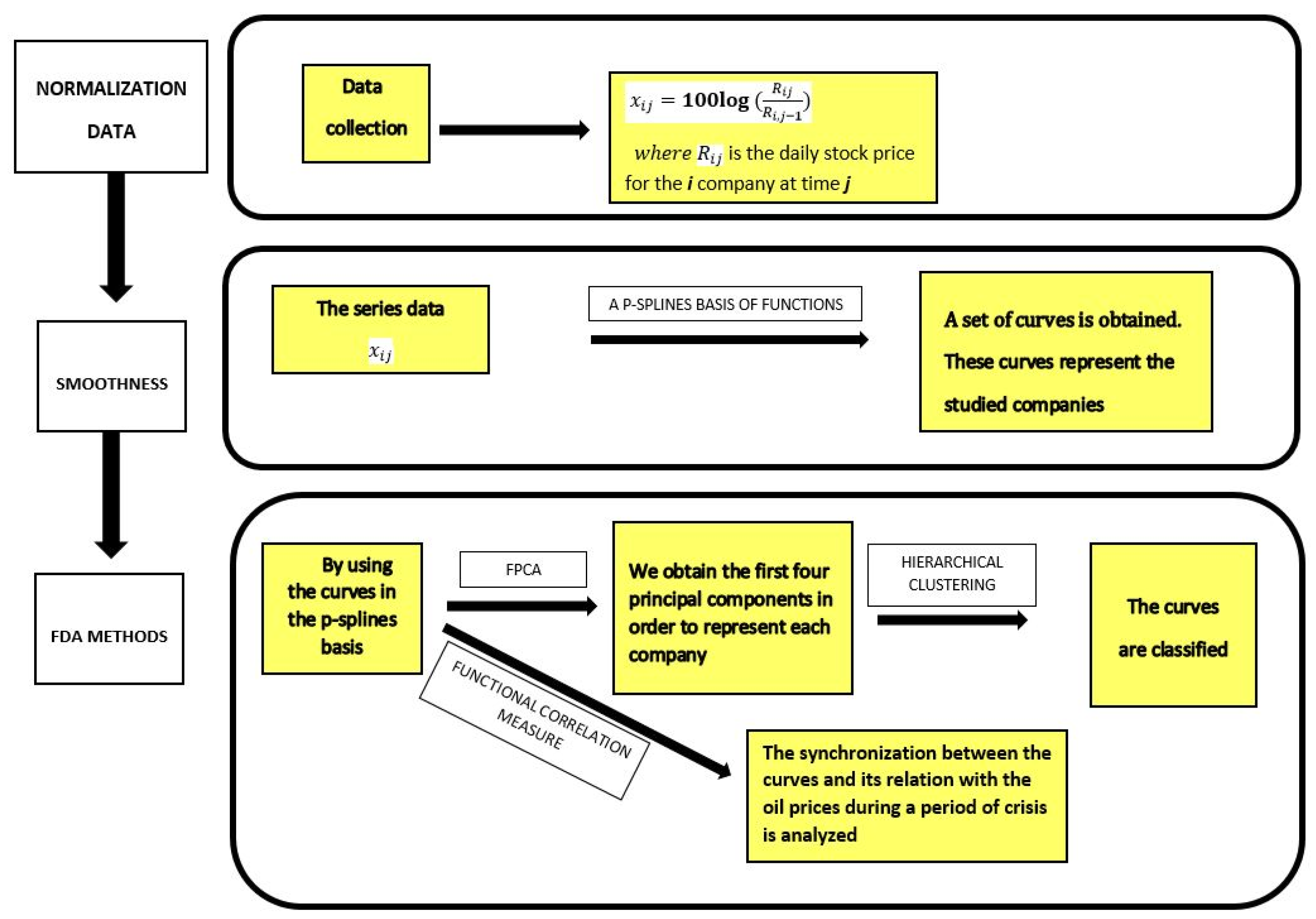
The first step in the data processing was the data normalizing into log returns

$${\mathit{x}}_{\mathit{i}\mathit{j}}=100log\left({\displaystyle \frac{{\mathit{R}}_{\mathit{i}\mathit{j}}}{{\mathit{R}}_{\mathit{i}, \mathit{j}-1}}}\right),$$

(1)

where ${\mathit{R}}_{\mathit{i}\mathit{j}}$ is the daily stock price $for the \mathit{i} company at time \mathit{j}.$

3.1.1. Smoothing Procedure

Once the data were transformed into cumulative log returns, the process of estimating and analyzing the functional data began. Although FDA aims to study the selected dynamic data and has different objectives than time series analysis, the two approaches complement each other. To achieve a satisfactory result in the FDA analysis, the curves must be smooth, belong to a vector space of real functions, be square-integrable, and be defined on a bounded interval τ = [0, T] [7].

Given a curve sample, $\mathit{X}=({\mathit{x}}_1\left(\mathit{t}\right)$, ${\mathit{x}}_2\left(\mathit{t}\right), \dots , {\mathit{x}}_{\mathit{N}}\left(\mathit{t}\right)$) the classical concepts of mean and variances in statistics are defined in [7]:

$$\overline{x}\left(\mathit{t}\right)={\displaystyle \frac{1}{\mathit{N}}}{{\displaystyle \sum }}_{\mathit{i}=1}^{\mathit{N}}{\mathit{x}}_i\left(\mathit{t}\right) \mathrm{and} va{r}_x\left(\mathit{t}\right)=\frac{1}{N-1}{\Sigma }_{\mathrm{i}=1}^N{\left(x_i\left(t\right)-\overline{x}\left(\mathit{t}\right)\right)}^2.$$

(2)

In our case, a discrete sample of the curves is given by the stock price returns of the companies under study. To reconstruct these curves, we employed a smoothing procedure that minimizes the mean squared error (MSE) between the original data points and the smoothed curves, using a basis of functions. The resulting curves must be analytical functions, requiring the continuity of its second derivative.

When functional data are used, it is crucial to select an appropriate basis of functions, guided by the nature of the functions under study. Typically, the Fourier basis is used for periodic functions, the splines basis for smooth functions, and the wavelets basis for curves characterized by multiple local features such as peaks or jumps. In this case, the spline’s basis is chosen. It is the most appropriate option due to the trend of the data and its lower MSE.

The smoothing procedure must consider two elements: the number of terms in the basis, K, and the value of the penalty of the smoothing parameter, λ. The role of this parameter is to strike a balance between data fit and curve smoothness. Ramsay and Silverman [7] demonstrate that the curves can be obtained by minimizing the expression:

$${{\displaystyle \sum }}_{j=1}^p{\left[x_{ij}-x_i\left(t_j\right)\right]}^2+\lambda {\displaystyle \int }{\left(D^2{x}_i\left(t\right)\right)}^{2}dt,$$

(3)

where $x_i=\left(x_{i1},x_{i2},\dots ,x_{ip}\right)$ is the vector of observed values at the days $t_1,t_2,\dots ,t_p$ and D is the differential operator.

The second term in this expression penalizes roughness by minimizing the value of the second derivative. There is no rule of thumb for determining the optimal value of λ. From the possible criteria, generalized cross validation (GCV) was chosen in this research. The optimal number of basic elements and the optimal smoothing parameter are obtained using the min.basis function. This function is implemented in the fda.usc package [31] for the R software. The min.basis function is based on the GCV method.

The series data in this work are processed taking into account the nature of the data. Figure 1 (similar to shown it in [15]) shows the methodology used in this paper.

3.1.2. Functional Correlation

In this section, the functional correlation measure introduced by Pérez et al. [32] is used.

Let two generic functions in the sample, $\mathrm{x}\left(t\right)$and $\mathrm{y}\left(t\right)$, defined in τ ≡ [0, T]. The following functional descriptive statistics over a functional data x are considered. These are:

$$\begin{gathered} {\mathrm{f}}_{\overline{\mathrm{x}}},f_{s^2},{\mathrm{f}}_{\mathrm{Sxy}} \in {\mathrm{L}}^2\left(\mathrm{\tau }\right), where f_{\overline{\mathrm{x}}}\left(\mathrm{t}\right)=\overline{\mathrm{x}\left(\mathrm{t}\right)}, f_{s^2}\left(t\right)=S_{x\left(t\right)}^2 \\ {\mathrm{f}}_{\mathrm{Sxy}}\left(t\right)={\mathrm{S}}_{x\left(t\right) y\left(t\right)}; \mathrm{for} \mathrm{all}\mathrm{t}\in \mathrm{\tau }, \\ \begin{array}{c}with \overline{\mathrm{x}\left(\mathrm{t}\right)}={\mathrm{T}}^{-1}·{{\displaystyle \int }}_0^{\mathrm{T}}\mathrm{x}\left(\mathrm{t}\right)\mathrm{dt}; S_{x\left(t\right)}^2={\mathrm{T}}^{-1}{{\displaystyle \int }}_0^T{\left(\mathrm{x}\left(\mathrm{t}\right)-\overline{\mathrm{x}\left(\mathrm{t}\right)}\right)}^2\mathrm{dt},\hfill \\ \mathrm{and} S_{x\left(t\right) y\left(t\right)}={\mathrm{T}}^{-1}{{\displaystyle \int }}_0^T\left(\mathrm{x}\left(\mathrm{t}\right)-\overline{\mathrm{x}\left(\mathrm{t}\right)}\right)\left(\mathrm{y}\left(\mathrm{t}\right)-\overline{\mathrm{y}\left(\mathrm{t}\right)}\right)\mathrm{dt}.\hfill \end{array} \end{gathered}$$

(4)

Then, the correlation value function ${\mathrm{f}}_{\mathrm{rxy} }\in { \mathrm{L}}^2\left(\mathrm{\tau }\right); {\mathrm{f}}_{\mathrm{rxy} }\left(t\right)={\mathrm{r}}_{x\left(t\right) y\left(t\right)}; \mathrm{for} \mathrm{all} \mathrm{t} \in \mathrm{\tau }$ with

$${\mathrm{r}}_{x\left(t\right) y\left(t\right)}={\displaystyle \frac{S_{x\left(t\right) y\left(t\right)}}{S_{x\left(t\right)}{S}_{y\left(t\right)}}}.$$

(5)

In this case, $\overline{\mathrm{x}\left(\mathrm{t}\right)}$ represents the average level of the element x(t) and $S_{x\left(t\right)}^2$ its variability over the average level. $S_{x\left(t\right) y\left(t\right)}$and ${\mathrm{r}}_{x\left(t\right) y\left(t\right)}$ measure the functional variability between the elements x(t) and y(t) (in the second case in a standardized way).

The measure ${\mathrm{r}}_{x\left(t\right) y\left(t\right)}$ is employed to establish a relation between the functional mean of BVC and the cumulative log returns of Brent curve. Moreover, it is used to validate a synchronization between the companies curves during a period of economic crisis. In this case, the crisis periods analyzed are the beginning of the COVID-19 crisis (between January 2020 and July 2020) and the drop in oil prices (due to the Russian invasion of Ukraine that began on 24 February 2022, which ends in August 2022).

3.1.3. K-Means Clustering

Similar to the methods proposed by Jacques and Preda [33] and Peng and Müler [34], this research proposes a two-stage classification method to group the curves according to its characteristics. In the first stage, the curves are classified into initial groups according to shared characteristics, establishing a reference framework for a more detailed analysis. For each curve, $x_i\left(t\right)$, a vector of coefficients ${\left(b_{i1},b_{i2},\dots ,b_{iJ}\right)}^T$ is obtained with respect to the first J basis functions. The first J basis functions accumulate a percentage of 90–95% of the total inertia. In the second stage, a k-means classification procedure is applied based on the vector of coefficients. In this stage, the groupings are refined, and the curves are assigned to more specific clusters, allowing for a more detailed classification of the return curves based on their behavior. This two-stage approach improves the robustness and accuracy of the curve clustering process.

3.1.4. Functional Principal Components Analysis

To identify the variables that explain the behavior of the curves, Functional Principal Component Analysis (FPCA) is recommended. FPCA is an extension of Principal Component Analysis (PCA) in multivariate statistical analyses. The eigenfunctions ${\xi }_j$ can be obtained by solving the Fredholm functional eigenequation:

$$\left(V\xi \right)\left(t\right)={{\displaystyle \int }}_0^{T}K\left(u,t\right)\xi \left(u\right)du=⟨K\left(t,.\right),\xi ⟩=\lambda \xi \left(t\right),$$

(6)

where $K\left(u,t\right)={\displaystyle \sum }_{i=1}^N{x}_i\left(u\right)x_i\left(t\right)$ is the kernel of the curves. The eigenfunctions, ${\xi }_j$, are orthogonal and each one is associated with an eigenvalue, ${\lambda }_j$. This eigenvalue represents the inertia of its eigenfunction. Mercer Theorem demonstrates that $K\left(u,t\right)$ can be written as:

$$K\left(u,t\right)={{\displaystyle \sum }}_{i=1}^{\infty }{\lambda }_i{\xi }_i\left(u\right){\xi }_i\left(t\right).$$

(7)

On the other hand, by following Karhunen–Loève’s procedure, any $x_i\left(t\right)$ function can be written as:

$$x_i\left(t\right)={{\displaystyle \sum }}_{j=1}^{\infty }{b}_{ij}{\xi }_j\left(t\right),$$

(8)

where the series converges in square mean in [0, T] and $b_{ij}$ are defined as:

$$b_{ij}=⟨{\xi }_j,x_i⟩={{\displaystyle \int }}_0^T{\xi }_j\left(t\right)x_i\left(t\right)dt,$$

(9)

where each $b_{ij}$ represents the projection of $x_i\left(t\right)$ in the j-th eigenfunction. In [7] it is shown that the eigenfunctions form an orthonormal basis for the space determined by the curves $x_i\left(t\right)$. Since the eigenfunctions are ordered by its inertia, a small number of them can collect a high percentage of information given in the curves $x_i\left(t\right)$.

If the curves belong to the same system, these curves share a number of common components. In this case, the first principal component shows the main trend of the pattern, while the second and subsequent components show the shape characteristics. The eigenfunctions help to identify different patterns of behavior in the group of curves.

3.2. Data Collection

In the data collection process for this study, meticulous criteria were used to select a total of twenty-six companies listed on the BVC. These companies were chosen based on specific attributes that made them relevant to the research objectives. In particular, the inclusion criteria were companies with a high trading volume, a dedicated approach to mitigating volatility, and efforts to reduce financing costs. In addition, these companies had extensive media coverage, which was essential for the exhaustive analysis of the dynamics of their market. The data collection phase was extended to cover a substantial period, encompassing 1535 daily observations of closing prices. This extensive period of time allowed the research to summarize a comprehensive view of market behavior. The data collection period began on 2 January 2017 and concluded on 20 April 2023.

The primary source of data for this study was the official website of the BVC, which serves as the authoritative platform for disseminating market-related information and statistics in the Colombian context. Furthermore, as oil prices play a pivotal role in the research, historical data pertaining to Brent crude oil, a key component of the study, was meticulously sourced from Investing.com, a recognized and reliable repository for financial and commodity data.

Table 1. Companies listed on the BVC in the period under review.

ABBR.	COMPANIES	SECTOR
1.EXI	ALMACENES EXITOS S.A.	Retail industry
2. DAV	BANCO DAVIVIENDA S.A.	Financial
3.BBO	BANCO DE BOGOTA S.A.	Financial
4.BCOL	BANCOLOMBIA S.A.	Financial
5.BVC	BOLSA DE VALORES COLOMBIANA S.A.	Financial
6.CNE	CANACOL ENERGY LTD	Energy
7.CEL	CELSIA S.A. E.S.P.	Energy
8.CEM	CEMENTOS ARGOS S.A.	Construction
9.COND	CONSTRUCCIONES EL CONDOR S.A.	Construction
10.CONC	CONCONCRETO	Construction
11.CFC	CORPORACIÓN FINANCIERA COLOMBIANA S.A.	Financial
12.ECO	ECOPETROL S.A.	Energy
13.GEB	GRUPO ENERGÍA BOGOTÁ S.A. E.S.P.	Energy
14.ARG	GRUPO ARGOS S.A.	Energy
15.GAV	GRUPO AVAL ACCIONES Y VALORES S.A.	Financial
16.ISA	INTERCONEXION ELECTRICA S.A. E.S.P.	Communications
17.ETB	EMPRESA DE TELECOMUNICACIONES DE BOGOTA S.A. E.S.P.	Communications
18.NUT	GRUPO NUTRESA S.A.	Nutrition
19.GSU	GRUPO DE INVERSIONES SURAMERICANA S.A.	Financial
20.MAS	MINEROS S.A.	Industrial
21.PMG	PROMIGAS	Energy
22.TPL	ORGANIZACIÓN TERPEL S.A.	Energy
23.ICO	FONDO BURSATIL ISHARES COLCAP	Financial
24.APR	ACERIAS PAZ DEL RIO S.A.	Industrial
25.HCOL	FONDO BURSATIL HORIZONS COLOMBIA	Financial
26.GBO	GRUPO BOLIVAR S.A.	Financial

provides an informative compilation of the companies that were considered in this study, along with their corresponding abbreviations and sectors, thereby enhancing the transparency and comprehensibility of the research dataset.

4. Results

The main objective of this work is to show the strong relation between oil prices and the Colombian stock market through Functional Data Analysis (FDA). The researchers aimed to discern how oil price shifts influenced daily closing prices in the Colombian stock market by using FDA methods. The investigation also sought to categorize curves with similar performance during the study period using FPCA and hierarchical clustering techniques.

4.1. Functional Data Processing

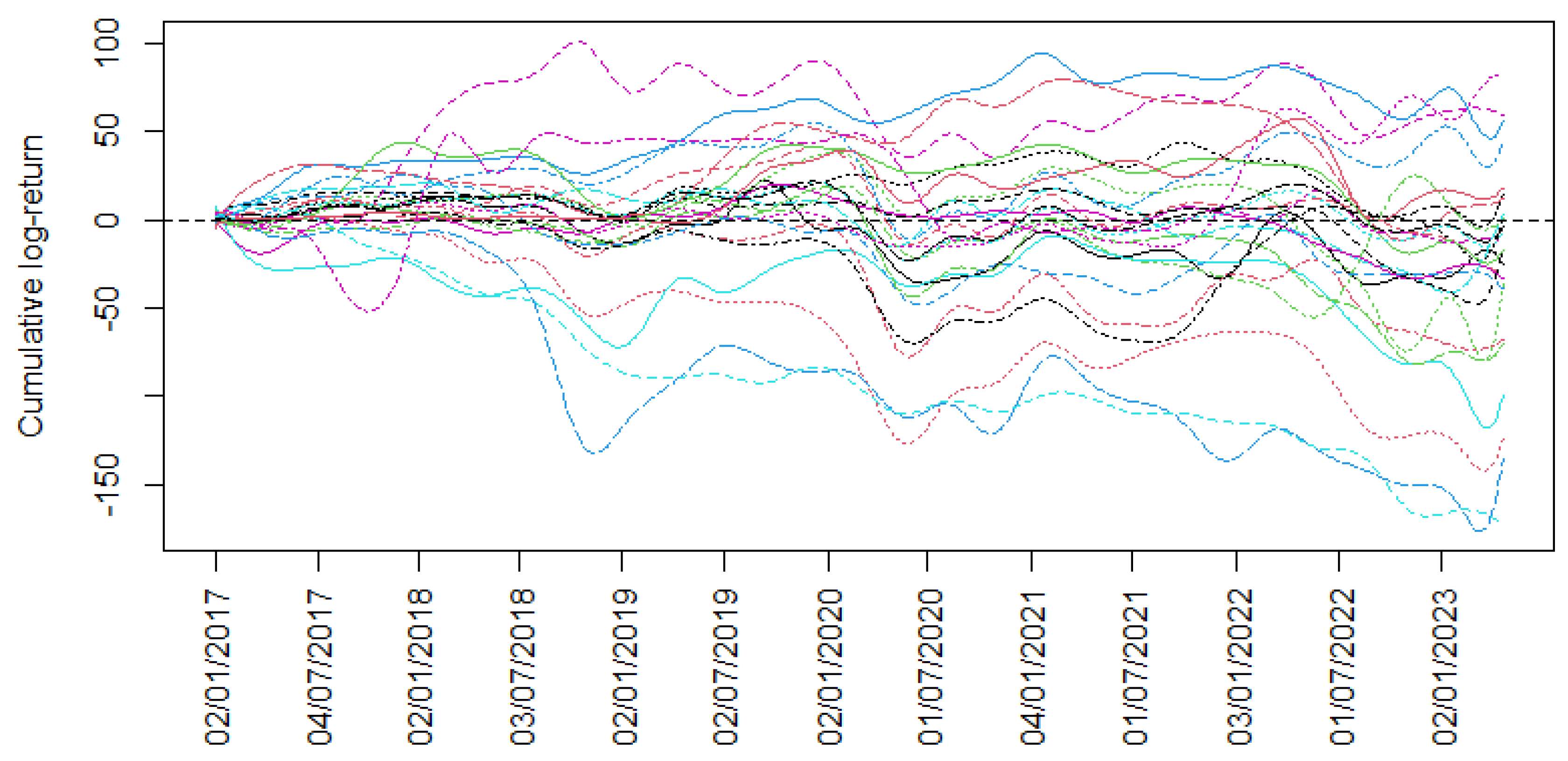
From the data available for the 26 companies listed on the Colombian Stock Exchange from 2 January 2017 to 20 April 2023, the cumulative logarithmic returns were calculated. Figure 2 shows the cumulative logarithmic returns series data about these companies.

In order to obtain the functional data, the P-splines basis was chosen. The optimal number of elements in the basis and the optimal smoothing parameter were obtained using the min.basis function in the fda.usc package in R 4.1.1 software. Figure 3 shows the functional data obtained with the optimal parameters.

Figure 4 shows the velocity curves defined as:

$$x{\prime }_i\left(t\right)={\displaystyle \frac{d{x}_i\left(t\right)}{dt}}.$$

(10)

The analyzed crisis periods are framed in this figure. Greater synchronization between the curves can be seen in both periods.

From the curves we now define the Estimated Functional Volatility of the stock market (EFV) as the mean of the sample velocity curves obtained from (2):

$$EFV\left(\mathit{t}\right)=\frac{1}{\mathit{N}}{{\displaystyle \sum }}_{\mathit{i}=1}^{\mathit{N}}\mathit{x}{\prime }_{\mathit{i}}\left(\mathit{t}\right).$$

(11)

Figure 5 shows the EFV of the BVC. The bands in the graph are given according to the Equation (4) by:

$$\overline{ \mathrm{x} \prime \left(\mathrm{t}\right)}\pm s_{x^{\prime }\left(t\right)} and \overline{ \mathrm{x} \prime \left(\mathrm{t}\right)}\pm 2s_{x^{\prime }\left(t\right)}$$

These bands determine medium, high and very high volatility levels. This depends on whether the EFV of the BVC is within the first band, between the first and second bands or outside the second band. Figure 5 shows two periods of very high volatility, marked between vertical lines. These periods coincide with the crisis periods analyzed, the COVID-19 crisis and the beginning of the invasion in Ukraine.

4.2. Functional Correlation

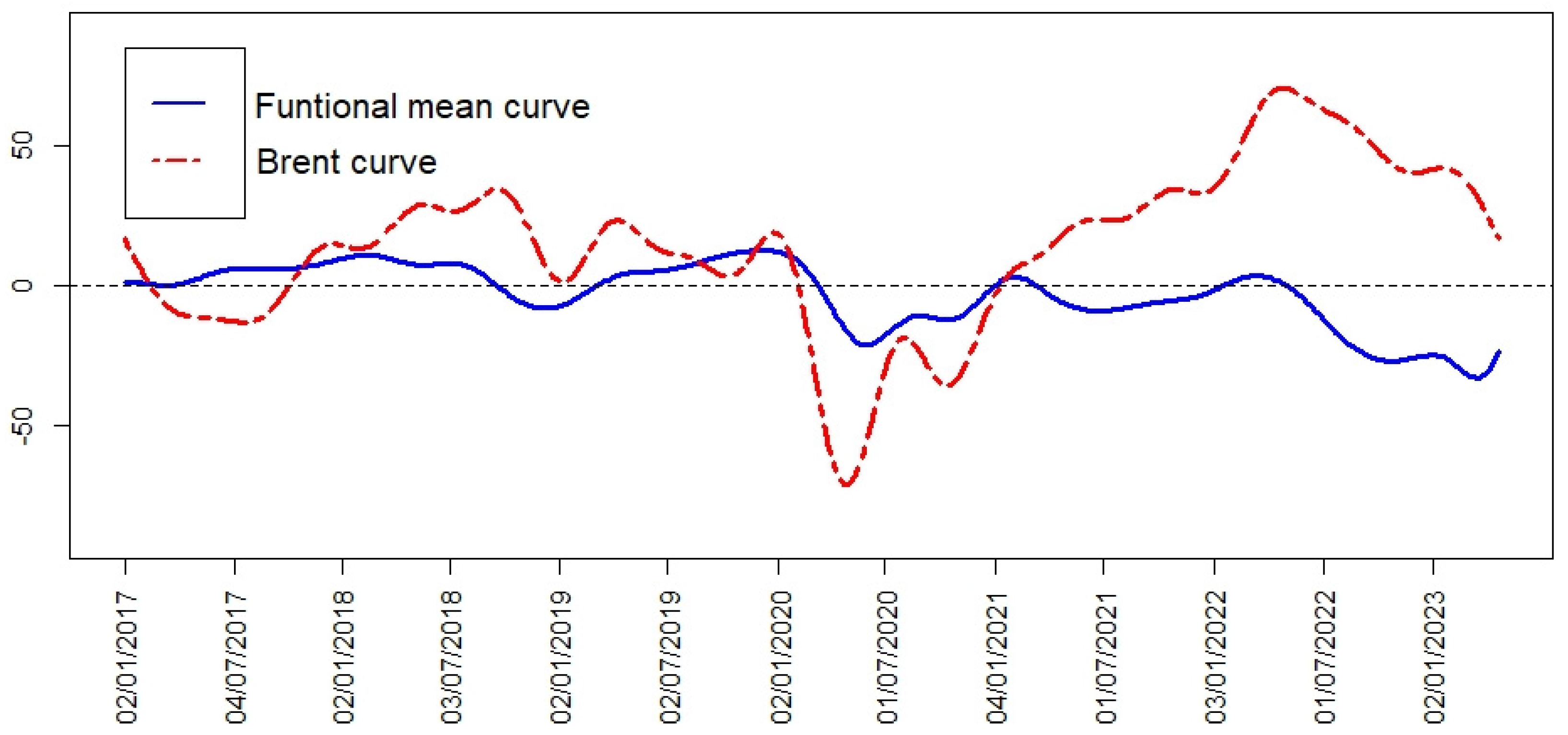
In Figure 6, the functional mean of the BVC’s curves and the cumulative log returns of Brent can be seen. The functional mean shows two declines, one at the beginning of 2020 and the other in 2022. The first decrease was caused by the COVID-19 pandemic, which forced governments to lock down their population and led to a collapse in the oil price. In the period of the second event (which coincides with the Russian invasion of Ukraine), a strong correlation with the oil price is shown (see Figure 6 and

Table 2. Functional correlation measured between the functional mean of BVC curves and the cumulative log returns of Brent in three different periods of time, the two crisis periods and the complete time period.

	Complete Time Period	COVID-19	UKRAINE
Functional correlation	−0.058	0.921	0.956

). In this time period, the oil price had a significant decline, which directly affected the Colombian market.

Table 2 shows an extremely large significant increase in the correlation measure the relation between the Functional mean of BVC and the cumulative log returns of Brent curves during the two crisis periods considered.

On the other hand, in order to validate a synchronization between the companies’ curves during a period of economic crisis, the functional correlation mean of each company to the others is calculated in two crisis periods and in the complete time period (

Table 3. For each company, the functional correlation mean to the other companies is calculated. This measure has been calculated in the two crisis periods and in the complete time period.

Company	Complete Time Period	COVID-19	UKRAINE
EXI	0.490	0.769	0.847
DAV	0.424	0.895	0.851
BBO	0.503	0.880	0.850
BCOL	0.329	0.896	0.901
BVC	0.497	0.778	0.910
CNE	0.442	0.856	0.884
CEL	0.521	0.894	0.869
CEM	0.511	0.895	0.908
COND	0.226	0.833	0.845
CONC	0.487	0.896	0.867
CFC	0.472	0.889	0.909
ECO	0.271	0.894	0.863
GEB	0.393	0.769	0.902
ARG	0.530	0.890	0.779
GAV	0.539	0.891	0.864
ISA	0.421	0.411	0.902
ETB	0.496	0.874	0.791
NUT	0.398	0.870	0.556
GSU	0.420	0.887	0.299
MAS	0.393	0.331	0.908
PMG	0.429	0.867	0.882
TPL	0.473	0.831	0.797
ICO	0.471	0.896	0.910
APR	0.258	0.568	0.817
HCOL	0.435	0.896	0.908
GBO	0.349	0.890	0.905
Mean	0.43	0.84	0.82

). The considered periods are, firstly, the COVID-19 crisis period and secondly, the beginning of the invasion of Ukraine.

Table 3 shows high correlations between almost all companies in crisis periods. Only in the initial period of COVID-19, the companies ISA and MAS do not show such a high correlation with the rest of the companies, while, in the Ukraine crisis, the companies GSU and NUT are the only ones that show low correlation values.

4.3. FPCA and Hierarchical Clustering

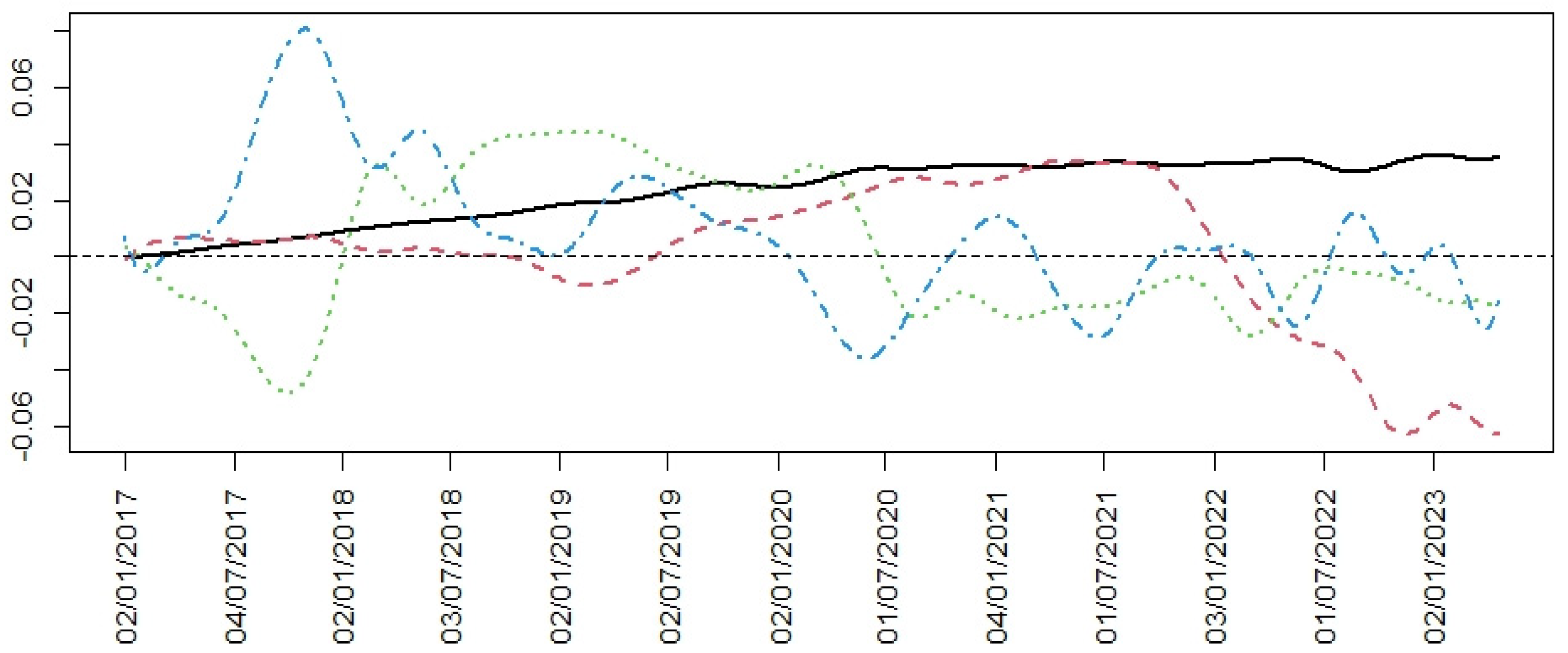
FPCA is a useful tool to identify components that explain the behavior of the set of curves. Figure 7 shows the first four principal components of the FPCA procedure. In this case, the first four Principal Components account for over 85.8%, 6.8%, 3.2%, and 1.4%, respectively, of the total explained variability. The first component, which shows the size of the data, shows a smooth linear growth until the first months of 2020. Subsequently, the trend is towards growth. The second component presents a cycle of variability whose critical points are February 2019 and July 2021.

As mentioned above, the coefficients of the curves in the basis, consisting of the principal components, provide a good linear representation of the curves. In this case, for each value, the vector formed by the coefficients of the first four principal components is considered. These components account for over 98.9% of the total inertia.

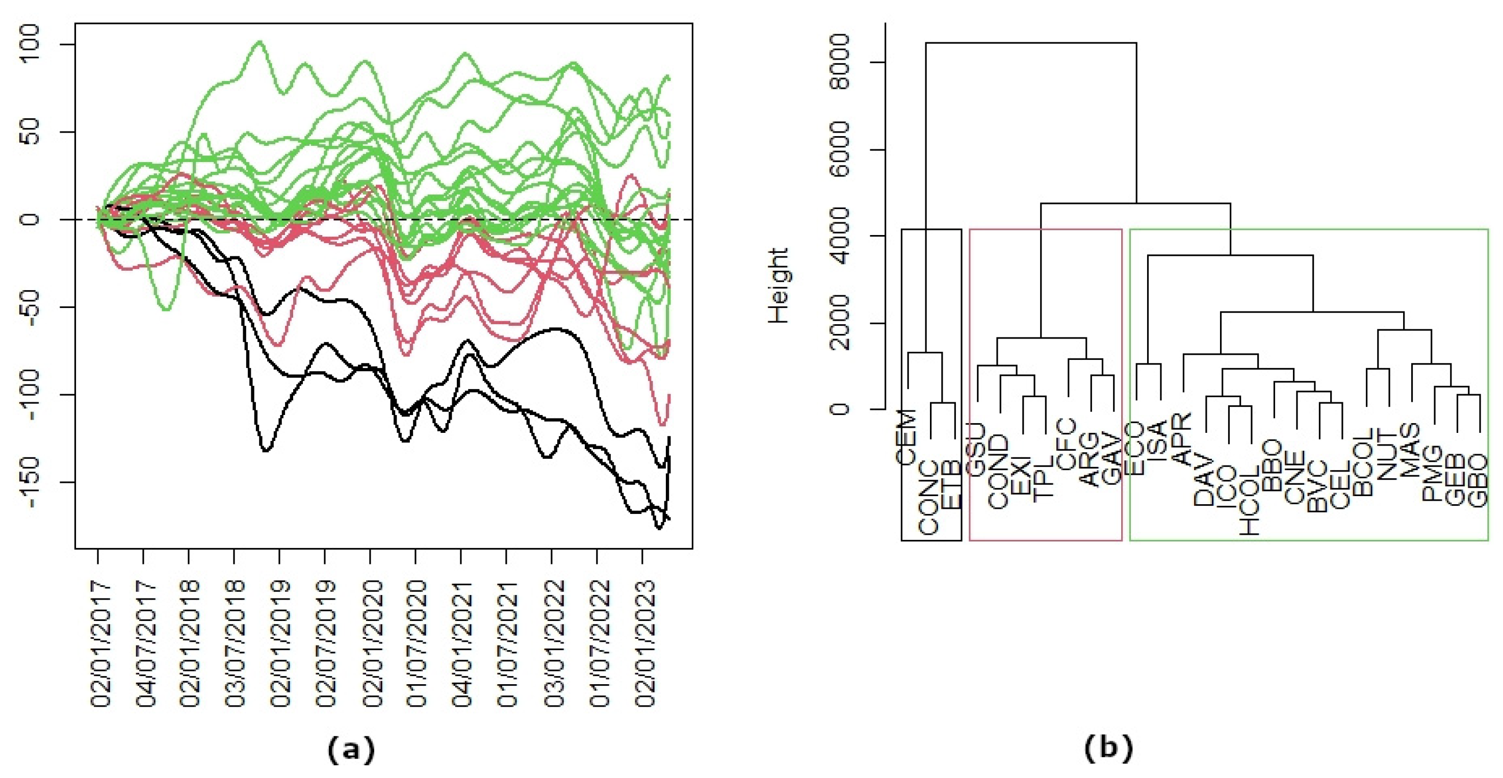
A hierarchical clustering method is applied to obtain a classification (Figure 8). The hierarchical clustering approach provided insights into three distinct groups of curves with similar trends, enhancing the understanding of market dynamics. The three companies, Argos Cements, Conconcreto (two of the three existing companies in the construction sector), and ETB (in the communications sector), belonging to the first group present extreme behavior and suffer the greatest devaluation. The second group, consisting of seven companies, is affected by fluctuations in oil prices. Two of these companies are in the energy sector, three are financial companies, another one is a construction company, and the last one belongs to retail sales. These companies present a consistent performance on the stock exchange and low volatility during the study period. Finally, the third group consists of sixteen companies whose stock market returns indicate a significant upward trend at the end of the time period. In this group, there are seven financial companies, five energy companies, two industrial companies, one communications company, and another company belonging to the food sector.

In Figure 9, we can see the mean curves of each group in Figure 8. The curve in the black color represents the companies with long-term losses, the curve in the red color is companies with middle gains, close to zero, and the curve in the green color is the group of companies with more gains.

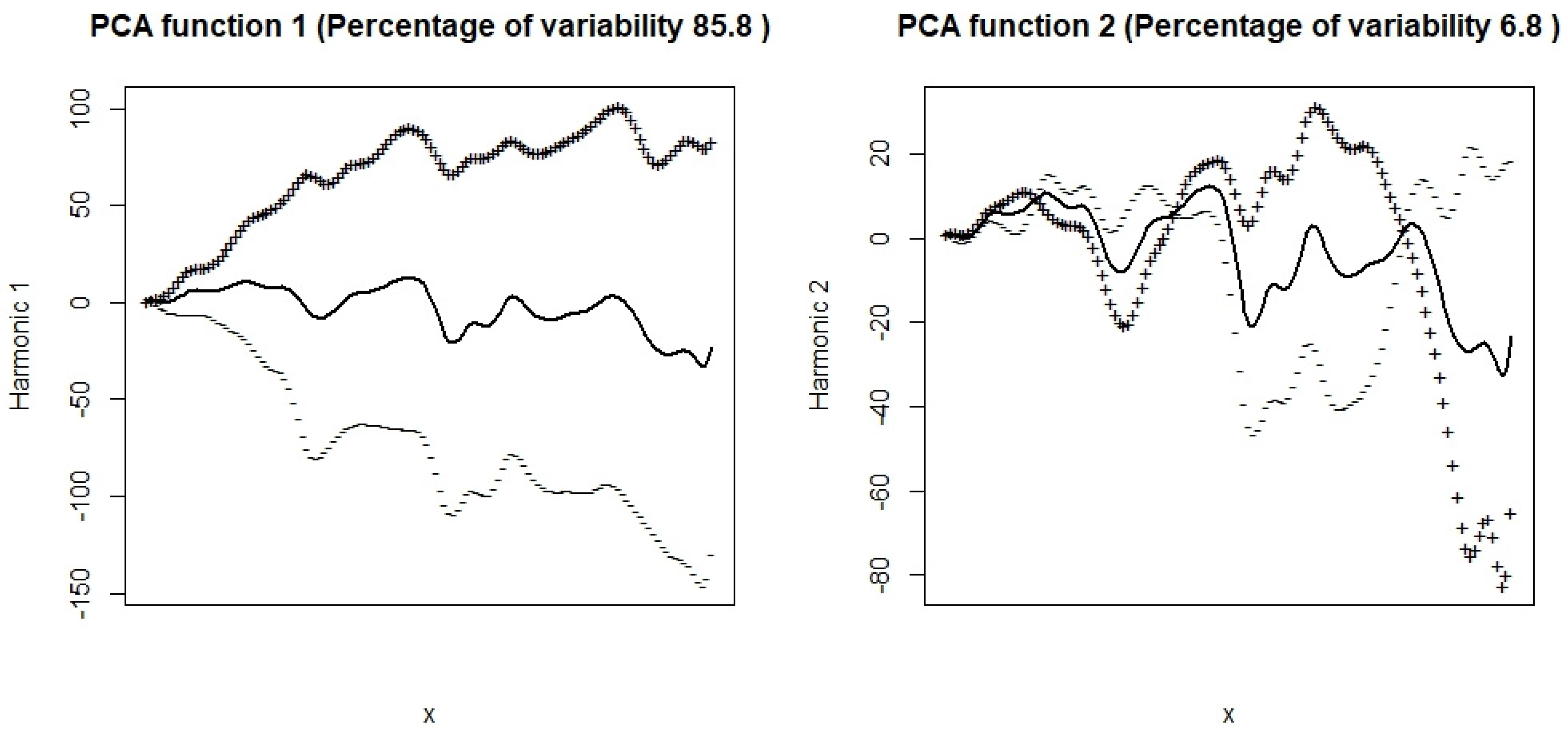
The two principal components are illustrated in Figure 10. These components are the perturbations of their mean function by adding and subtracting a multiple of each principal component. As in the vectorial case, the first principal component, which accounts for over 85.8% of the inertia, is a component of the size that shows the variation of the prices; thus, it explains the behavior in the long term of BVC. On the other hand, the second principal component, which accounts for over 6.8% of the variability, shows the market’s response to the crises of COVID-19 and the war in Ukraine because this component changes direction and makes the positive and negative disturbances permute. Therefore, the losses become the profits and vice versa. Ingrassia and Costanzo [12] interpret this component as a “shock” since the shares that had a good (resp. bad) performance before March 2022 have been going down (resp. rising) after that date.

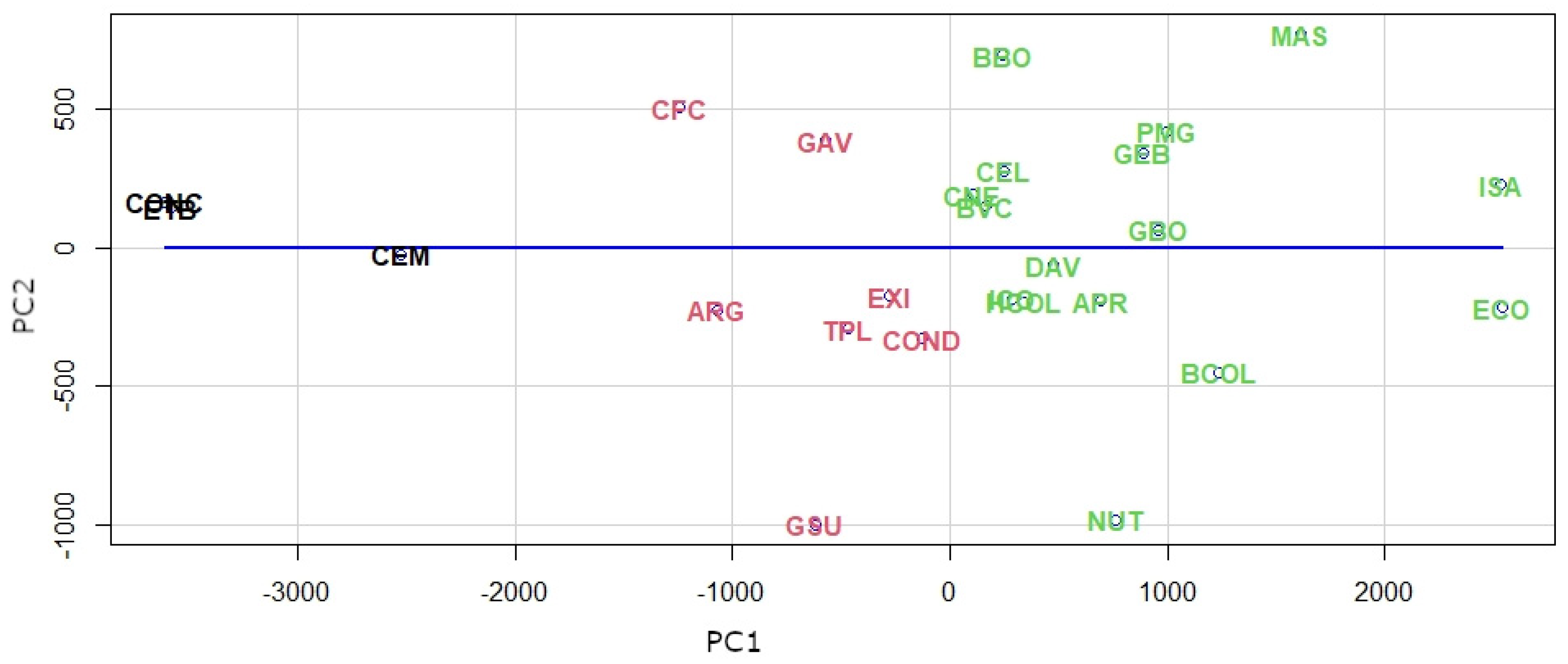
In Figure 11, we consider the projections of the four principal components of the two first ones, and it is possible to see the groups of companies represented in Figure 8. The first group, in the black color, represents the companies with low values in the first component, that is, the companies with long-term losses. The second group, in the red color, with middle values in the first component, are companies with gains close to zero. The third group, in the green color, are companies with high values in the first component, that is, the companies with more long-term gains.

5. Discussion

By using a basis of P-splines, we have transformed the time series of 26 relevant stock markets in BVC into curves with good metric and analytical properties. By applying functional statistical analysis techniques to the curves obtained, we have gone from working in a high-frequency discrete multivariate space to working in an infinite-dimensional functional Hilbert space with a metric induced by the L² norm. The FDA has provided us with the necessary tools. That is, the basic descriptive techniques, the correlation analysis between curves, the functional principal component analysis, and the functional cluster analysis. With these tools, we have been able to obtain the above results.

From the point of view of managing the information provided by the BVC sample, the conversion into functions is both a limitation and a strength. It is a limitation because smoothing involves a correction of the daily closing prices of the stock market, and it is a strength because these closing values are still indicators of the behavior of the stock market during a trading day. Furthermore, while the analysis of time series requires the condition of stationarity that forces transformations to be made in the data, the FDA does not require any previous condition.

The first derivative of the curves provides us with the instantaneous rates of change in stock prices over the entire period considered. The analysis of the velocities offers us a novel perspective on stock market volatility and has allowed us, through the EFV measure, to identify two of the most important crises suffered by humanity in recent years as periods of high volatility.

We propose in future research to validate whether this procedure is valid for other stock markets and during other crises. Moreover, given the importance of the concept of volatility in economics, it would be interesting to introduce, starting from the EFV measure, other measures of functional volatility and to study their theoretical properties.

The functional correlations have allowed us to analyze the relationship between the average values of the BVC, both through a global indicator and in windows of the total period considered. By using FPCA, we have transformed the total variability of the values analyzed into orthogonal components. These components explain specific aspects of market behavior and how periods of crisis affect it. Finally, through the cluster analysis carried out on the first components, which account for 99% of the total variability, we have classified the values into groups with a pre-established degree of homogeneity.

One of the limitations of the study is that the decision on the number of clusters is certainly subjective, given the descriptive nature of this multivariate technique. However, the reader can examine the dendrogram in Figure 8b together with the projection on the plane of the first two components in Figure 11 to make his or her own interpretation. For example, a cut at a distance of 2000 units in the dendrogram would leave the first two clusters the same but would divide the third into three, which, as a matter of note, would isolate the two best-performing stocks in the BVC, Ecopetrol, and Interconexión Electrica S.A.

6. Conclusions

The main objective of this work is to identify and quantify the consequences of COVID-19 and the war in Ukraine on the BVC. The graphical analysis of the information provided by the 26 most important stocks of the BVC has allowed us to identify a synchronization effect of the velocity curves in the crisis periods. This indicates that the stocks reacted in a similar way to the strategies of the operators, who acted in a scenario of great uncertainty. To confirm this assessment, we have verified that, for each company, the functional correlation mean to the other companies increases significantly in the two crisis periods, going from an average value of 0.43 in the entire period to 0.84 and 0.82 in the crisis periods, respectively.

We have found an extremely significant increase in the functional correlation between the mean curve of the stock market and the Brent oil price curve in the total period considered in the two crisis periods. Hence, this increase goes from functional incorrelation (r = −0.05) in the entire study period to levels above 0.9 in each of the crisis periods.

In this work, we have introduced the Estimated Functional Volatility (EFV) curve. This curve is defined as the average of the derivatives curves in the studied period. The EFV graph shows how, in the two crisis periods considered, the distance between this curve and the line that represents zero volatility is bigger than two typical deviations, maintaining high volatility levels.

FPCA is a useful tool to identify components that explain the behavior of the set of curves. In this case, the four first principal components account for over 98.9% of the total inertia. As in the vectorial case, the first principal component, which accounts for over 85.8% of the inertia, is a component of size that shows the variation of the prices and, thus, explains the behavior in the long term of BVC. On the other hand, the second principal component, which accounts for over 6.8% of the variability, shows the market’s response to the crises of COVID-19 and the war in Ukraine because this component changes direction and makes the positive and negative disturbances permute. Therefore, the losses become the profits and vice versa. Most likely, approximately 7% of the variability that explains the third and fourth components will be justified by regional or Colombian state causes.

The hierarchical clustering enables us to understand the market dynamics because it classifies the values of BVC into three distinct groups of curves with similar trends. The three companies in the first group suffer the greatest devaluation. This group consists of two companies in the construction sector and one company in the communication sector. The second group consists of seven companies: two in the financial sector, two in the energy sector, three in the financial sector, another one in the construction sector, and the last one belongs to retail sales. These companies present a consistent performance on the stock exchange and low volatility during the study period. Finally, the third group consists of sixteen companies whose stock market returns indicate a significant upward trend at the end of the time period. In this group, there are seven financial companies, five energy companies, two industrial companies, one communications company, and another company belonging to the food sector.

In conclusion, we think that this work shows the usefulness of the FDA as a complement to time series analysis in the study of stock markets.