On the Recursive Sequence $x_{n+1}=\frac{a{x}_{n-1}}{b+c{x}_n{x}_{n-1}}$

Abstract

In this paper, we investigate the dynamical behaviors of the rational difference equation $x_n=\left(a{x}_{n-1}\right)/\left(b+c{x}_n{x}_{n-1}\right)$ with arbitrary initial conditions, where a, b, and c are real numbers. A general solution is obtained. The asymptotic stability of the equilibrium points is investigated, using a nonlinear stability criterion combined with basin of attraction analysis and simulation to determine the stability regions of the equilibrium points. The existence of the periodic solutions is discussed. We investigate the codim-1 bifurcations of the equation. We show that the equation exhibits a Neimark–Sacker bifurcation. For this bifurcation, the topological normal form is computed. To confirm our theoretical results, we performed a numerical simulation as well as numerical bifurcation analysis by using the Matlab package MatContM.

1. Introduction

The study of difference equations has expanded significantly over the past decade. The reason for this is that these equations are used in modeling real-life problems in a wide range of fields of science. For example, in biology, these equations can be used in modeling some natural phenomena, such as the size of a population at time n, the blood cell production, and the propagation of annual plants, while in economics these equations have been used to study the pricing of a certain commodity and the national income of a country [1,2,3].

In this paper, we study the general solution and the dynamical behaviors of the rational difference equation

$$x_{n+1}={\displaystyle \frac{a{x}_{n-1}}{b+c{x}_n{x}_{n-1}}},n=0,1,\dots$$

(1)

where a, b, and c are real numbers with $bc>0$, and the initial conditions $x_{-1}$ and $x_0$ are real numbers. Also, we study the bifurcations that occur in this equation. Cinar [4] investigated the positive solutions of the rational difference equation

$$x_{n+1}={\displaystyle \frac{x_{n-1}}{1+x_n{x}_{n-1}}},n=0,1,\dots .$$

Cinar [5] investigated the solutions of the difference equation

$$x_{n+1}={\displaystyle \frac{x_{n-1}}{-1+a{x}_n{x}_{n-1}}},n=0,1,\dots ,$$

where $a>0$. Cinar [6] investigated the positive solutions of the difference equation

$$x_{n+1}={\displaystyle \frac{x_{n-1}}{1+a{x}_n{x}_{n-1}}},n=0,1,\dots ,$$

where $a>0$. Aloqeili [7] discussed the stability properties and semi-cycle behavior of the solution of the difference equation

$$x_{n+1}={\displaystyle \frac{x_{n-1}}{a-x_n{x}_{n-1}}},n=0,1,\dots ,$$

where $a>0$. Andruch-Sobi and Migda [8] investigated the asymptotic behavior of all solutions of the rational difference equation

$$x_{n+1}={\displaystyle \frac{a{x}_{n-1}}{b+c{x}_n{x}_{n-1}}},n=0,1,\dots$$

with a positive a and c, negative b, and non-negative initial conditions $x_{-1}$ and $x_0$. The same equation with a positive b was considered in [9]. Elsayed [10] obtained the solutions of the rational difference equation

$$x_{n+1}={\displaystyle \frac{x_{n-3}}{\pm 1\pm x_{n-1}{x}_{n-3}}},n=0,1,\dots .$$

Abo-Zeid [11] introduced the solutions of the rational difference equation

$$x_{n+1}={\displaystyle \frac{a{x}_{n-3}}{b+c{x}_{n-1}{x}_{n-3}}},n=0,1,\dots .$$

Ghazel et al. [12] obtained the solutions and the dynamical behaviors of the rational difference equation

$$x_{n+1}={\displaystyle \frac{C{x}_{n-5}}{A+B{x}_{n-2}{x}_{n-5}}},n=0,1,\dots .$$

Karatas et al. [13] investigated the positive solutions of the difference equation

$$x_{n+1}={\displaystyle \frac{x_{n-5}}{1+x_{n-2}{x}_{n-5}}},n=0,1,\dots .$$

Abo-Zeid [14] investigated the global behavior of all solutions of the rational difference equation

$$x_{n+1}={\displaystyle \frac{A{x}_{n-k}}{B+C{\displaystyle \prod _{i=0}^k}{x}_{n-i}}},n=0,1,\dots .$$

Karatas [15] obtained the solution of the rational difference equation

$$x_{n+1}={\displaystyle \frac{a{x}_{n-(2k+3)}}{-a\mp x_{n-(k+1)}{x}_{n-(2k+3)}}},n=0,1,\dots .$$

Karatas et al. [16] proved the global asymptotic stability of the equation

$${\displaystyle \frac{A{x}_{n-\left[2\right(k+j)+1]}}{B+C{x}_{n-(k+j)}{x}_{n-\left[2\right(k+j)+1]}}},n=0,1,\dots .$$

Moreover, they obtained the solutions of some special cases of this difference equation by applying the standard iteration method. The study of the dynamical behaviors of the solutions of rational difference equations, such as local and global stability, periodicity, and bifurcations, has been discussed by many authors—for examples, see [2,16,17,18,19,20,21] and the references therein.

The present paper is motivated by the incomplete analysis of Equation (1). We extend the work of [4,5,6,7,8,9] by studying its general form with a, b, and c as real numbers with $bc>0$, and the initial conditions being arbitrary real numbers. We perform a comprehensive stability analysis, considering not only the trivial equilibrium point and instability regions of other equilibrium points but also the stability regions of all equilibrium points of Equation (1). Furthermore, we investigate the existence of bifurcations in Equation (1). Importantly, previous studies have not addressed the bifurcation analysis of this equation. The setup of this paper is outlined as follows. In Section 2, we show that Equation (1) has only three equilibrium points. We discuss the stability of these points. We show that the equilibrium point ${\tilde{x}}_1$ is globally asymptotically stable (see also Section 3). On the other hand, we show that the equilibrium points ${\tilde{x}}_2$ and ${\tilde{x}}_3$ are never linearly stable. 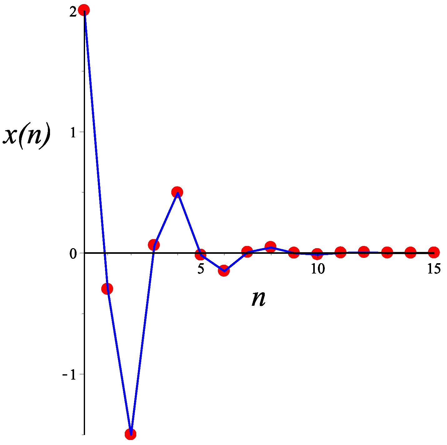In Section 3, we obtain the analytical solution of Equation (1). We prove that, if $(b/a)\in (-1,1)$, then every solution of Equation (1) converges to zero even if we choose negative initial conditions. Furthermore, we discuss the dynamic behaviors of the solution and the periodic solutions of Equation (1). In Section 4, a complete bifurcation analysis is presented. We show that Equation (1) exhibits a Neimark–Sacker bifurcation. For this bifurcation, we compute the topological normal form. In Section 5, we use a nonlinear stability criterion to better understand the stability of the equilibrium points ${\tilde{x}}_2$ and ${\tilde{x}}_3$ where the characteristic equation evaluated at these points always has one root less than one and the other is equal to −1. This criterion is based on stability analysis in the direction of the eigenvector corresponding to the eigenvalue equal to −1. We show that these points are stable and we always have small regions of stability in their domain. In Section 6, we perform a numerical simulation as well as a numerical bifurcation analysis to confirm our theoretical results.

2. Preliminaries

Here, we present some known results that will be useful in the study of Equation (1). Let $I\subseteq \mathbb{R}$ and let $f:I^{k+1}⟶I$ be a continuously differentiable function. Then, for any initial conditions $x_{-k},x_{-k+1},\dots ,x_0\in I$, the difference equation

$$x_{n+1}=f(x_n,x_{n-1},\dots ,x_{n-k}),n=0,1,\dots .$$

(2)

has a unique solution ${\left\{x_n\right\}}_{n=-k}^{\infty }$.

Definition 1.

A point $\tilde{x}$ is called an equilibrium point of Equation (2) if $f(\tilde{x},\tilde{x},\dots ,\tilde{x})=\tilde{x}$.

Definition 2.

A solution ${\left\{x_n\right\}}_{n=-k}^{\infty }$ is said to be periodic with period t if

$$x_{n+t}=x_n\mathit{for}\mathit{all}n\ge -k.$$

(3)

A solution ${\left\{x_n\right\}}_{n=-k}^{\infty }$ is called periodic with prime period t if t is the smallest positive integer for which Equation (3) holds.

Definition 3.

Let $\tilde{x}$ be an equilibrium point of Equation (2).

1. 

$\tilde{x}$ is called stable if for every $\epsilon >0$, there exists $\delta >0$ such that for all $x_{-k},x_{-k+1},\dots ,x_0\in I$ and ${\displaystyle \sum _{j=0}^k}\left|x_{-k+j}-\tilde{x}\right|<\delta$, we have $\left|x_n-\tilde{x}\right|<\epsilon$, for all $n\ge -k$.

2. 

$\tilde{x}$ is called locally asymptotically stable if $\tilde{x}$ is stable and there exists $\gamma >0$, such that for all $x_{-k},x_{-k+1},\dots ,x_0\in I$ and ${\displaystyle \sum _{j=0}^k}\left|x_{-k+j}-\tilde{x}\right|<\gamma$, we have $\underset{n\to \infty }{lim}{x}_n=\tilde{x}$.

3. 

$\tilde{x}$ is called a global attractor if for all $x_{-k},x_{-k+1},\dots ,x_0\in I$, we have $\underset{n\to \infty }{lim}{x}_n=\tilde{x}$.

4. 

$\tilde{x}$ is called globally asymptotically stable if $\tilde{x}$ is stable and is a global attractor.

5. 

$\tilde{x}$ is called unstable if $\tilde{x}$ is not stable.

Let

$$y_{n+1}=\sum _{j=0}^k{\displaystyle \frac{\mathrm{\partial }f(\tilde{x},\tilde{x},\dots ,\tilde{x})}{\mathrm{\partial }{x}_{n-j}}}{y}_{n-j},n=0,1,\dots$$

(4)

where the function f is given in Equation (2) and $\tilde{x}$ is an equilibrium point of Equation (2). Equation (4) is the linearized equation of Equation (2) about $\tilde{x}$. The characteristic equation of Equation (4) is

$${\lambda }^{k+1}-\sum _{j=0}^k{\displaystyle \frac{\mathrm{\partial }f(\tilde{x},\tilde{x},\dots ,\tilde{x})}{\mathrm{\partial }{x}_{n-j}}}{\lambda }^{k-j}=0.$$

(5)

Theorem 1.

Assume that f is a continuously differentiable function and let $\tilde{x}$ be an equilibrium point of Equation (2). Then, the following statements are true.

1. 

$\tilde{x}$ is locally asymptotically stable if all roots of Equation (5) (i.e., the eigenvalues) have absolute value less than 1.

2. 

$\tilde{x}$ is unstable if at least one root of Equation (5) has an absolute value greater than 1.

The change in variables $x_n\mapsto \sqrt{(b/c)}{x}_n$ (with $bc>0$) reduces the Equation (1) to the rational difference equation

$$x_{n+1}={\displaystyle \frac{\alpha x_{n-1}}{1+x_n{x}_{n-1}}},n=0,1,\dots$$

(6)

where $\alpha =a/b$.

Theorem 2.

Equation (6) has exactly three equilibrium points, which are given by

$${\tilde{x}}_1=0\mathit{when}\alpha \in \mathbb{R},{\tilde{x}}_2=\sqrt{\alpha -1}\mathit{when}\alpha >1,{\tilde{x}}_3=\sqrt{\alpha -1}\mathit{when}\alpha >1.$$

Proof. 

For the equilibrium points of Equation (6), we can write $\tilde{x}=\left(\alpha \tilde{x}\right)/(1+\tilde{x}\tilde{x})$. Then, we have $\tilde{x}\left[{\tilde{x}}^2-(\alpha -1)\right]=0$. Therefore, the equilibrium points of Equation (6) are ${\tilde{x}}_1=0$ when $\alpha \in \mathbb{R}$ and ${\tilde{x}}_{2,3}=\pm \sqrt{\alpha -1}$ when $\alpha >1$. □

The linearized equation associated with Equation (6) about the equilibrium point $\tilde{x}$ is given by the linear difference equation:

$$y_{n+1}={\displaystyle \frac{\mathrm{\partial }f}{\mathrm{\partial }{x}_{n-1}}}(\tilde{x},\tilde{x})y_{n-1}+{\displaystyle \frac{\mathrm{\partial }f}{\mathrm{\partial }{x}_n}}(\tilde{x},\tilde{x})y_n={\displaystyle \frac{\alpha }{{\left(1+{\tilde{x}}^2\right)}^2}}{y}_{n-1}-{\displaystyle \frac{\alpha {\tilde{x}}^2}{{\left(1+{\tilde{x}}^2\right)}^2}}{y}_n.$$

(7)

The characteristic equation corresponding to Equation (7) is

$${\lambda }^2+{\displaystyle \frac{\alpha {\tilde{x}}^2}{{\left(1+{\tilde{x}}^2\right)}^2}}\lambda -{\displaystyle \frac{\alpha }{{\left(1+{\tilde{x}}^2\right)}^2}}=0.$$

(8)

The following corollary directly follows from Theorem 1.

Corollary 1.

If $\alpha \in (-1,1)$, then the equilibrium point ${\tilde{x}}_1$ of Equation (6) is locally asymptotically stable.

Note that, for the equilibrium points ${\tilde{x}}_{2,3}$, the characteristic Equation (8) has two eigenvalues, namely ${\lambda }_1=-1$ and ${\lambda }_2={\displaystyle \frac{1}{\alpha }}<1$ for all $\alpha >1$. Since there is always one root equal to $|{\lambda }_1|=1$, then the equilibrium point is never locally asymptotically stable. The stability analysis of the equilibrium points ${\tilde{x}}_2$ and ${\tilde{x}}_3$ will be discussed in Section 5.

3. Analytical Expression of ${\left\{x_n\right\}}_{n=1}^{\infty }$

In the following, we obtain the analytical expression of the general solution ${\left\{x_n\right\}}_{n=1}^{\infty }$ of Equation (6) with arbitrary initial conditions $x_{-1}$ and $x_0$, where $\alpha$ is a real number.

Theorem 3.

Let $x_{-1}$ and $x_0$ be real numbers and ${\left\{x_n\right\}}_{n=1}^{\infty }$ be a solution of Equation (6). Then, for $n=1,2,\dots$, all solutions of Equation (6) are of the form

$$x_n=\left\{\begin{array}{ccc}{\displaystyle \frac{{\alpha }^{n/2}{x}_0{\displaystyle \prod _{j=0}^{(n/2)-1}}\left(1+x_0{x}_{-1}{\displaystyle \sum _{k=0}^{2j}}{\alpha }^k\right)}{{\displaystyle \prod _{j=0}^{(n/2)-1}}\left(1+x_0{x}_{-1}{\displaystyle \sum _{k=0}^{2j+1}}{\alpha }^k\right)}}\hfill & \mathit{if}\hfill & n\mathit{is}\mathit{even}\hfill \\ \hfill \\ {\displaystyle \frac{{\alpha }^{(n+1)/2}{x}_{-1}{\displaystyle \prod _{j=0}^{\left(\right(n+1)/2)-1}}\left(1+x_0{x}_{-1}{\displaystyle \sum _{k=0}^{2j-1}}{\alpha }^k\right)}{{\displaystyle \prod _{j=0}^{\left(\right(n+1)/2)-1}}\left(1+x_0{x}_{-1}{\displaystyle \sum _{k=0}^{2j}}{\alpha }^k\right)}}\hfill & \mathit{if}\hfill & n\mathit{is}\mathit{odd}\hfill \end{array}\right.$$

(9)

Proof. 

Assume that n is even. Therefore, $n-1$ and $n+1$ are odd. Substituting Equation (9) into the L.H.S of Equation (6) gives

$$x_{n+1}={\displaystyle \frac{{\alpha }^{n/2+1}{x}_{-1}{\displaystyle \prod _{j=0}^{n/2}}\left(1+x_0{x}_{-1}{\displaystyle \sum _{k=0}^{2j-1}}{\alpha }^k\right)}{{\displaystyle \prod _{j=0}^{n/2}}\left(1+x_0{x}_{-1}{\displaystyle \sum _{k=0}^{2j}}{\alpha }^k\right)}}.$$

(10)

On the other hand, substituting Equation (9) into the R.H.S of Equation (6) gives

$$\begin{array}{cc}{\displaystyle \frac{\alpha x_{n-1}}{1+x_n{x}_{-1}}}\hfill & ={\displaystyle \frac{{\displaystyle \frac{{\alpha }^{n/2+1}{x}_{-1}{\displaystyle \prod _{j=0}^{(n/2)-1}}\left(1+x_0{x}_{-1}{\displaystyle \sum _{k=0}^{2j-1}}{\alpha }^k\right)}{{\displaystyle \prod _{j=0}^{(n/2)-1}}\left(1+x_0{x}_{-1}{\displaystyle \sum _{k=0}^{2j}}{\alpha }^k\right)}}}{1+x_0{x}_{-1}{\alpha }^n{\displaystyle \frac{{\displaystyle \prod _{j=0}^{(n/2)-1}}\left(1+x_0{x}_{-1}{\displaystyle \sum _{k=0}^{2j}}{\alpha }^k\right)}{{\displaystyle \prod _{j=0}^{(n/2)-1}}\left(1+x_0{x}_{-1}{\displaystyle \sum _{k=0}^{2j+1}}{\alpha }^k\right)}}{\displaystyle \frac{{\displaystyle \prod _{j=0}^{(n/2)-1}}\left(1+x_0{x}_{-1}{\displaystyle \sum _{k=0}^{2j-1}}{\alpha }^k\right)}{{\displaystyle \prod _{j=0}^{(n/2)-1}}\left(1+x_0{x}_{-1}{\displaystyle \sum _{k=0}^{2j}}{\alpha }^k\right)}}}}\hfill \\ \hfill \\ & ={\displaystyle \frac{{\displaystyle \frac{{\alpha }^{n/2+1}{x}_{-1}{\displaystyle \prod _{j=0}^{(n/2)-1}}\left(1+x_0{x}_{-1}{\displaystyle \sum _{k=0}^{2j-1}}{\alpha }^k\right)}{{\displaystyle \prod _{j=0}^{(n/2)-1}}\left(1+x_0{x}_{-1}{\displaystyle \sum _{k=0}^{2j}}{\alpha }^k\right)}}}{1+x_0{x}_{-1}{\alpha }^n{\displaystyle \frac{{\displaystyle \prod _{j=0}^{(n/2)-1}}\left(1+x_0{x}_{-1}{\displaystyle \sum _{k=0}^{2j-1}}{\alpha }^k\right)}{{\displaystyle \prod _{j=0}^{(n/2)-1}}\left(1+x_0{x}_{-1}{\displaystyle \sum _{k=0}^{2j+1}}{\alpha }^k\right)}}}}={\displaystyle \frac{{\displaystyle \frac{{\alpha }^{n/2+1}{x}_{-1}{\displaystyle \prod _{j=0}^{(n/2)-1}}\left(1+x_0{x}_{-1}{\displaystyle \sum _{k=0}^{2j-1}}{\alpha }^k\right)}{{\displaystyle \prod _{j=0}^{(n/2)-1}}\left(1+x_0{x}_{-1}{\displaystyle \sum _{k=0}^{2j}}{\alpha }^k\right)}}}{1+x_0{x}_{-1}{\alpha }^n{\displaystyle \frac{1}{\left(1+x_0{x}_{-1}{\displaystyle \sum _{k=0}^{n-1}}{\alpha }^k\right)}}}}\hfill \\ \hfill \\ & ={\displaystyle \frac{{\displaystyle \frac{{\alpha }^{n/2+1}{x}_{-1}{\displaystyle \prod _{j=0}^{(n/2)-1}}\left(1+x_0{x}_{-1}{\displaystyle \sum _{k=0}^{2j-1}}{\alpha }^k\right)}{{\displaystyle \prod _{j=0}^{(n/2)-1}}\left(1+x_0{x}_{-1}{\displaystyle \sum _{k=0}^{2j}}{\alpha }^k\right)}}}{{\displaystyle \frac{1+x_0{x}_{-1}{\displaystyle \sum _{k=0}^{n-1}}{\alpha }^k+x_0{x}_{-1}{\alpha }^n}{\left(1+x_0{x}_{-1}{\displaystyle \sum _{k=0}^{n-1}}{\alpha }^k\right)}}}}={\displaystyle \frac{{\alpha }^{n/2+1}{x}_{-1}{\displaystyle \prod _{j=0}^{(n/2)-1}}\left(1+x_0{x}_{-1}{\displaystyle \sum _{k=0}^{2j-1}}{\alpha }^k\right)}{{\displaystyle \prod _{j=0}^{(n/2)-1}}\left(1+x_0{x}_{-1}{\displaystyle \sum _{k=0}^{2j}}{\alpha }^k\right)}}{\displaystyle \frac{\left(1+x_0{x}_{-1}{\displaystyle \sum _{k=0}^{n-1}}{\alpha }^k\right)}{\left(1+x_0{x}_{-1}{\displaystyle \sum _{k=0}^n}{\alpha }^k\right)}}\hfill \\ \hfill \\ & ={\displaystyle \frac{{\alpha }^{n/2+1}{x}_{-1}{\displaystyle \prod _{j=0}^{n/2}}\left(1+x_0{x}_{-1}{\displaystyle \sum _{k=0}^{2j-1}}{\alpha }^k\right)}{{\displaystyle \prod _{j=0}^{n/2}}\left(1+x_0{x}_{-1}{\displaystyle \sum _{k=0}^{2j}}{\alpha }^k\right)}}=x_{n+1}.\hfill \end{array}$$

Similarly, if we assume that n is odd, then $n-1$ and $n+1$ are even. If we substitute Equation (9) into the L.H.S of Equation (6), we obtain

$$x_{n+1}={\displaystyle \frac{{\alpha }^{(n+1)/2}{x}_0{\displaystyle \prod _{j=0}^{\left(\right(n+1)/2)-1}}\left(1+x_0{x}_{-1}{\displaystyle \sum _{k=0}^{2j}}{\alpha }^k\right)}{{\displaystyle \prod _{j=0}^{\left(\right(n+1)/2)-1}}\left(1+x_0{x}_{-1}{\displaystyle \sum _{k=0}^{2j+1}}{\alpha }^k\right)}}.$$

(11)

From the R.H.S of Equation (6), it follows that

$$\begin{array}{cc}{\displaystyle \frac{\alpha x_{n-1}}{1+x_n{x}_{-1}}}\hfill & ={\displaystyle \frac{{\displaystyle \frac{{\alpha }^{(n+1)/2}{x}_0{\displaystyle \prod _{j=0}^{\left(\right(n-1)/2)-1}}\left(1+x_0{x}_{-1}{\displaystyle \sum _{k=0}^{2j}}{\alpha }^k\right)}{{\displaystyle \prod _{j=0}^{\left(\right(n-1)/2)-1}}\left(1+x_0{x}_{-1}{\displaystyle \sum _{k=0}^{2j+1}}{\alpha }^k\right)}}}{1+x_0{x}_{-1}{\alpha }^n{\displaystyle \frac{{\displaystyle \prod _{j=0}^{\left(\right(n+1)/2)-1}}\left(1+x_0{x}_{-1}{\displaystyle \sum _{k=0}^{2j-1}}{\alpha }^k\right)}{{\displaystyle \prod _{j=0}^{\left(\right(n+1)/2)-1}}\left(1+x_0{x}_{-1}{\displaystyle \sum _{k=0}^{2j}}{\alpha }^k\right)}}{\displaystyle \frac{{\displaystyle \prod _{j=0}^{\left(\right(n-1)/2)-1}}\left(1+x_0{x}_{-1}{\displaystyle \sum _{k=0}^{2j}}{\alpha }^k\right)}{{\displaystyle \prod _{j=0}^{\left(\right(n-1)/2)-1}}\left(1+x_0{x}_{-1}{\displaystyle \sum _{k=0}^{2j+1}}{\alpha }^k\right)}}}}\hfill \\ \hfill \\ & ={\displaystyle \frac{{\displaystyle \frac{{\alpha }^{(n+1)/2}{x}_0{\displaystyle \prod _{j=0}^{\left(\right(n-1)/2)-1}}\left(1+x_0{x}_{-1}{\displaystyle \sum _{k=0}^{2j}}{\alpha }^k\right)}{{\displaystyle \prod _{j=0}^{\left(\right(n-1)/2)-1}}\left(1+x_0{x}_{-1}{\displaystyle \sum _{k=0}^{2j+1}}{\alpha }^k\right)}}}{1+x_0{x}_{-1}{\alpha }^n{\displaystyle \frac{{\displaystyle \prod _{j=0}^{\left(\right(n-1)/2)-1}}\left(1+x_0{x}_{-1}{\displaystyle \sum _{k=0}^{2j}}{\alpha }^k\right)}{{\displaystyle \prod _{j=0}^{\left(\right(n+1)/2)-1}}\left(1+x_0{x}_{-1}{\displaystyle \sum _{k=0}^{2j}}{\alpha }^k\right)}}}}={\displaystyle \frac{{\displaystyle \frac{{\alpha }^{(n+1)/2}{x}_0{\displaystyle \prod _{j=0}^{\left(\right(n-1)/2)-1}}\left(1+x_0{x}_{-1}{\displaystyle \sum _{k=0}^{2j}}{\alpha }^k\right)}{{\displaystyle \prod _{j=0}^{\left(\right(n-1)/2)-1}}\left(1+x_0{x}_{-1}{\displaystyle \sum _{k=0}^{2j+1}}{\alpha }^k\right)}}}{1+x_0{x}_{-1}{\alpha }^n{\displaystyle \frac{1}{\left(1+x_0{x}_{-1}{\displaystyle \sum _{k=0}^{n-1}}{\alpha }^k\right)}}}}\hfill \\ \hfill \\ & ={\displaystyle \frac{{\displaystyle \frac{{\alpha }^{(n+1)/2}{x}_0{\displaystyle \prod _{j=0}^{\left(\right(n-1)/2)-1}}\left(1+x_0{x}_{-1}{\displaystyle \sum _{k=0}^{2j}}{\alpha }^k\right)}{{\displaystyle \prod _{j=0}^{\left(\right(n-1)/2)-1}}\left(1+x_0{x}_{-1}{\displaystyle \sum _{k=0}^{2j+1}}{\alpha }^k\right)}}}{{\displaystyle \frac{1+x_0{x}_{-1}{\displaystyle \sum _{k=0}^{n-1}}{\alpha }^k+x_0{x}_{-1}{\alpha }^n}{\left(1+x_0{x}_{-1}{\displaystyle \sum _{k=0}^{n-1}}{\alpha }^k\right)}}}}={\displaystyle \frac{{\alpha }^{(n+1)/2}{x}_0{\displaystyle \prod _{j=0}^{\left(\right(n-1)/2)-1}}\left(1+x_0{x}_{-1}{\displaystyle \sum _{k=0}^{2j}}{\alpha }^k\right)}{{\displaystyle \prod _{j=0}^{\left(\right(n-1)/2)-1}}\left(1+x_0{x}_{-1}{\displaystyle \sum _{k=0}^{2j+1}}{\alpha }^k\right)}}{\displaystyle \frac{\left(1+x_0{x}_{-1}{\displaystyle \sum _{k=0}^{n-1}}{\alpha }^k\right)}{\left(1+x_0{x}_{-1}{\displaystyle \sum _{k=0}^n}{\alpha }^k\right)}}\hfill \\ \hfill \\ & ={\displaystyle \frac{{\alpha }^{(n+1)/2}{x}_0{\displaystyle \prod _{j=0}^{\left(\right(n+1)/2)-1}}\left(1+x_0{x}_{-1}{\displaystyle \sum _{k=0}^{2j}}{\alpha }^k\right)}{{\displaystyle \prod _{j=0}^{\left(\right(n+1)/2)-1}}\left(1+x_0{x}_{-1}{\displaystyle \sum _{k=0}^{2j+1}}{\alpha }^k\right)}}=x_{n+1}.\hfill \end{array}$$

This completes the proof. □

Theorem 4.

Let $\alpha \in (-1,1)$. Then, every solution $\left\{x_n\right\}$ of Equation (6) converges to zero.

Proof. 

Let $\left\{x_n\right\}$ be a solution of Equation (2) with the initial conditions $x_{-1}$ and $x_0$ being real numbers. If $x_{-1}=x_0=0$, then it is clear that $x_n=0$ for all $n\ge 1$. If $x_0=0$ and $x_{-1}\ne 0$, then we can easily obtain that

$$x_n=\left\{\begin{array}{ccc}0\hfill & \mathrm{if}\hfill & n\mathrm{is}\mathrm{even}\hfill \\ \hfill \\ x_{-1}{\alpha }^{(n+1)/2}\hfill & \mathrm{if}\hfill & n\mathrm{is}\mathrm{odd}\hfill \end{array}\right.$$

Since $\alpha \in (-1,1)$, it is clear that $\underset{n\to \infty }{lim}{x}_n=0$. Similarly, if $x_{-1}=0$ and $x_0\ne 0$, then we can easily obtain that

$$x_n=\left\{\begin{array}{ccc}{x}_0{\alpha }^{n/2}\hfill & \mathrm{if}\hfill & n\mathrm{is}\mathrm{even}\hfill \\ \hfill \\ 0\hfill & \mathrm{if}\hfill & n\mathrm{is}\mathrm{odd}\hfill \end{array}\right.$$

Hence, $\underset{n\to \infty }{lim}{x}_n=0$ for all $\alpha \in (-1,1)$. If $x_{-1}\ne 0$ and $x_0\ne 0$, then let $x_{-1}{x}_0\ne 0$. It is enough to show that the sub-sequences $\left\{x_{2n}\right\}$ and $\left\{x_{2n-1}\right\}$ converge to 0 as $n\to \infty$. From Equation (9), we obtain

$$\begin{array}{cc}|x_{2n}|\hfill & =\left|x_0{\alpha }^n{\displaystyle \frac{{\displaystyle \prod _{j=0}^{n-1}}\left(1+x_0{x}_{-1}{\displaystyle \sum _{k=0}^{2j}}{\alpha }^k\right)}{{\displaystyle \prod _{j=0}^{n-1}}\left(1+x_0{x}_{-1}{\displaystyle \sum _{k=0}^{2j+1}}{\alpha }^k\right)}}\right|=\left|x_0{\alpha }^n{\displaystyle \frac{{\displaystyle \prod _{j=0}^{n-1}}\left(1+x_0{x}_{-1}{\displaystyle \sum _{k=0}^{2j}}{\alpha }^k\right)}{{\displaystyle \prod _{j=0}^{n-1}}\left(1+x_0{x}_{-1}{\displaystyle \sum _{k=0}^{2j}}{\alpha }^k+x_0{x}_{-1}{\alpha }^{2j+1}\right)}}\right|\hfill \\ & =|x_0{\alpha }^n|\exp \left({\displaystyle \sum _{j=0}^{n-1}}ln\left({\displaystyle \frac{1+x_0{x}_{-1}{\displaystyle \sum _{k=0}^{2j}}{\alpha }^k}{1+x_0{x}_{-1}{\displaystyle \sum _{k=0}^{2j}}{\alpha }^k+x_0{x}_{-1}{\alpha }^{2j+1}}}\right)\right)\hfill \\ & =|x_0{\alpha }^n|\exp \left(ln\left({\displaystyle \frac{{\displaystyle \prod _{j=0}^{n-1}}\left(1+x_0{x}_{-1}{\displaystyle \sum _{k=0}^{2j}}{\alpha }^k\right)}{{\displaystyle \prod _{j=0}^{n-1}}\left(1+x_0{x}_{-1}{\displaystyle \sum _{k=0}^{2j}}{\alpha }^k+x_0{x}_{-1}{\alpha }^{2j+1}\right)}}\right)\right)\hfill \\ & =|x_0{\alpha }^n|\exp \left({\displaystyle \sum _{j=0}^{n-1}}ln\left({\displaystyle \frac{1}{{\displaystyle \frac{1+x_0{x}_{-1}{\displaystyle \sum _{k=0}^{2j}}{\alpha }^k+x_0{x}_{-1}{\alpha }^{2j+1}}{1+x_0{x}_{-1}{\displaystyle \sum _{k=0}^{2j}}{\alpha }^k}}}}\right)\right)\hfill \\ & =|x_0{\alpha }^n|\exp \left({\displaystyle \sum _{j=0}^{n-1}}ln\left({\displaystyle \frac{1}{1+r\left(j\right)}}\right)\right),\mathrm{where}r\left(j\right)={\displaystyle \frac{x_0{x}_{-1}{\alpha }^{2j+1}}{1+x_0{x}_{-1}{\displaystyle \sum _{k=0}^{2j}}{\alpha }^k}},\hfill \\ & =|x_0{\alpha }^n|\exp \left({\displaystyle \sum _{j=0}^{n-1}}ln\left(-\left(1+r\left(j\right)\right)\right)\right)=\left|x_0{\alpha }^n\right|\exp \left({\displaystyle \sum _{j=0}^{n-1}}ln\left(1-\left(2+r\left(j\right)\right)\right)\right)\hfill \\ & \le |x_0{\alpha }^n|\exp \left(-{\displaystyle \sum _{j=0}^{n-1}}\left(2+r\left(j\right)\right)\right)=|x_0{\alpha }^n|\exp \left(-2n-{\displaystyle \sum _{j=0}^{n-1}}r\left(j\right)\right)=\left|x_0{\alpha }^n\right|\exp (-2n)\exp \left(-{\displaystyle \sum _{j=0}^{n-1}}r\left(j\right)\right).\hfill \end{array}$$

For $\alpha \in (-1,1)$, $r\left(j\right)={\displaystyle \frac{x_0{x}_{-1}{\alpha }^{2j+1}}{1+x_0{x}_{-1}{\displaystyle \sum _{k=0}^{2j}}{\alpha }^k}}={\displaystyle \frac{x_0{x}_{-1}{\alpha }^{2j+1}(\alpha -1)}{x_0{x}_{-1}{\alpha }^{2j+1}-x_0{x}_{-1}+\alpha -1}}$, then $\underset{j\to \infty }{lim}\left|{\displaystyle \frac{r(j+1)}{r\left(j\right)}}\right|=\left|{\alpha }^2\right|<1$, and hence the series ${\displaystyle \sum _{j=0}}r\left(j\right)$ is convergent. Therefore,

$$|x_0{\alpha }^n|\exp (-2n)\exp \left(-{\displaystyle \sum _{j=0}^{n-1}}r\left(j\right)\right)\to 0\mathrm{as}n\to \infty ,$$

so $\left|x_{2n}\right|\to 0$ as $n\to \infty$ and hence $\left\{x_{2n}\right\}\to 0$ as $n\to \infty$.

Similarly, we obtain

$$\begin{array}{cc}|x_{2n-1}|\hfill & =\left|x_{-1}{\alpha }^n\right|{\displaystyle \frac{{\displaystyle \prod _{j=0}^{n-1}}\left(1+x_0{x}_{-1}{\displaystyle \sum _{k=0}^{2j-1}}{\alpha }^k\right)}{{\displaystyle \prod _{j=0}^{n-1}}\left(1+x_0{x}_{-1}{\displaystyle \sum _{k=0}^{2j}}{\alpha }^k\right)}}=\left|x_0{\alpha }^n\right|\exp \left({\displaystyle \sum _{j=0}^{n-1}}ln\left({\displaystyle \frac{1}{1+s\left(j\right)}}\right)\right),\mathrm{where}s\left(j\right)={\displaystyle \frac{x_0{x}_{-1}{\alpha }^{2j}}{1+x_0{x}_{-1}{\displaystyle \sum _{k=0}^{2j-1}}{\alpha }^k}}\hfill \\ & \le |x_0{\alpha }^n|\exp (-2n)\exp \left(-{\displaystyle \sum _{j=0}^{n-1}}s\left(j\right)\right).\hfill \end{array}$$

For $\alpha \in (-1,1)$, $s\left(j\right)={\displaystyle \frac{x_0{x}_{-1}{\alpha }^{2j}}{1+x_0{x}_{-1}{\displaystyle \sum _{k=0}^{2j-1}}{\alpha }^k}}={\displaystyle \frac{x_0{x}_{-1}{\alpha }^{2j}(\alpha -1)}{x_0{x}_{-1}{\alpha }^{2j}-x_0{x}_{-1}+\alpha -1}}$, then ${\displaystyle \underset{j\to \infty }{lim}}\left|{\displaystyle \frac{s(j+1)}{s\left(j\right)}}\right|=\left|{\alpha }^2\right|<1$, and hence the series ${\displaystyle \sum _{j=0}}s\left(j\right)$ is convergent. Therefore,

$$|x_0{\alpha }^n|\exp (-2n)\exp \left(-{\displaystyle \sum _{j=0}^{n-1}}s\left(j\right)\right)\to 0\mathrm{as}n\to \infty ,$$

so $\left\{x_{2n-1}\right\}\to 0$ as $n\to \infty$. This completes the proof. □

Theorem 5.

If $\alpha \in (-1,1)$, then the equilibrium point ${\tilde{x}}_1$ of Equation (6) is globally asymptotically stable.

Proof. 

It follows from Theorem 4 and Corollary 1. □

Theorem 6.

If $x_{-1}=x_0=\xi \in \mathbb{R}$ and $\alpha ={\xi }^2+1$, then the solution $\left\{x_n\right\}$ of Equation (6) is equal to ξ.

Proof. 

If $x_{-1}=x_0=\xi$ and $\alpha ={\xi }^2+1$, we want to show that $x_{2n}=x_{2n-1}=\xi$ for all $n\ge 1$. Using Equation (9),

$$\begin{array}{cc}\hfill x_{2n}& ={\displaystyle \frac{{\left({\xi }^2+1\right)}^n\xi {\displaystyle \prod _{j=0}^{n-1}}\left(1+{\xi }^2{\displaystyle \frac{{({\xi }^2+1)}^{2j+1}-1}{\left({\xi }^2+1\right)-1}}\right)}{{\displaystyle \prod _{j=0}^{n-1}}\left(1+{\xi }^2{\displaystyle \frac{{({\xi }^2+1)}^{2j+2}-1}{\left({\xi }^2+1\right)-1}}\right)}}={\displaystyle \frac{{\left({\xi }^2+1\right)}^n\xi {\displaystyle \prod _{j=0}^{n-1}}{\left({\xi }^2+1\right)}^{2j+1}}{{\displaystyle \prod _{j=0}^{n-1}}{\left({\xi }^2+1\right)}^{2j+2}}}\hfill \\ & ={\displaystyle \frac{{\left({\xi }^2+1\right)}^n\xi {\displaystyle \prod _{j=0}^{n-1}}{\left({\xi }^2+1\right)}^{2j+1}}{{\displaystyle \prod _{j=0}^{n-1}}\left({\xi }^2+1\right){\displaystyle \prod _{j=0}^{n-1}}{\left({\xi }^2+1\right)}^{2j+1}}}={\displaystyle \frac{{\left({\xi }^2+1\right)}^n\xi }{{\left({\xi }^2+1\right)}^n}}=\xi .\hfill \end{array}$$

Similarly,

$$\begin{array}{cc}\hfill x_{2n-1}& ={\displaystyle \frac{{\left({\xi }^2+1\right)}^n\xi {\displaystyle \prod _{j=0}^{n-1}}\left(1+{\xi }^2{\displaystyle \frac{{({\xi }^2+1)}^{2j}-1}{\left({\xi }^2+1\right)-1}}\right)}{{\displaystyle \prod _{j=0}^{n-1}}\left(1+{\xi }^2{\displaystyle \frac{{({\xi }^2+1)}^{2j+1}-1}{\left({\xi }^2+1\right)-1}}\right)}}={\displaystyle \frac{{\left({\xi }^2+1\right)}^n\xi {\displaystyle \prod _{j=0}^{n-1}}{\left({\xi }^2+1\right)}^{2j}}{{\displaystyle \prod _{j=0}^{n-1}}{\left({\xi }^2+1\right)}^{2j+1}}}\hfill \\ & ={\displaystyle \frac{{\left({\xi }^2+1\right)}^n\xi {\displaystyle \prod _{j=0}^{n-1}}{\left({\xi }^2+1\right)}^{2j}}{{\displaystyle \prod _{j=0}^{n-1}}\left({\xi }^2+1\right){\displaystyle \prod _{j=0}^{n-1}}{\left({\xi }^2+1\right)}^{2j}}}={\displaystyle \frac{{\left({\xi }^2+1\right)}^n\xi }{{\left({\xi }^2+1\right)}^n}}=\xi .\hfill \end{array}$$

This completes the proof. □

Theorem 7.

The nontrivial solutions $\left\{x_n\right\}$ of Equation (6) will be periodic with period 2 if the initial conditions are chosen such that $x_{-1}\ne 0$, $x_0={\displaystyle \frac{\alpha -1}{x_{-1}}}$ and $\alpha \ne 1$. Then, $\left\{x_n\right\}=\left\{x_{-1},{\displaystyle \frac{\alpha -1}{x_{-1}}},x_{-1},{\displaystyle \frac{\alpha -1}{x_{-1}}},x_{-1},{\displaystyle \frac{\alpha -1}{x_{-1}}},\dots \right\}$.

Proof. 

If $x_{-1}\ne 0$, $x_0={\displaystyle \frac{\alpha -1}{x_{-1}}}$ and $\alpha \ne 1$, we want to show that $x_{2n}=x_0$ and $x_{2n-1}=x_{-1}$ for all $n\ge 1$. Using Equation (9),

$$x_{2n}={\displaystyle \frac{{\alpha }^n{x}_0{\displaystyle \prod _{j=0}^{n-1}}\left(1+\left(\alpha -1\right){\displaystyle \frac{{\alpha }^{2j+1}-1}{\alpha -1}}\right)}{{\displaystyle \prod _{j=0}^{n-1}}\left(1+\left(\alpha -1\right){\displaystyle \frac{{\alpha }^{2j+2}-1}{\alpha -1}}\right)}}={\displaystyle \frac{{\alpha }^n{x}_0{\displaystyle \prod _{j=0}^{n-1}}{\alpha }^{2j+1}}{{\displaystyle \prod _{j=0}^{n-1}}{\alpha }^{2j+2}}}={\displaystyle \frac{{\alpha }^n{x}_0{\displaystyle \prod _{j=0}^{n-1}}{\alpha }^{2j+1}}{{\displaystyle \prod _{j=0}^{n-1}}\alpha {\displaystyle \prod _{j=0}^{n-1}}{\alpha }^{2j+1}}}=x_0.$$

Similarly,

$$x_{2n-1}={\displaystyle \frac{{\alpha }^n{x}_{-1}{\displaystyle \prod _{j=0}^{n-1}}\left(1+\left(\alpha -1\right){\displaystyle \frac{{\alpha }^{2j}-1}{\alpha -1}}\right)}{{\displaystyle \prod _{j=0}^{n-1}}\left(1+\left(\alpha -1\right){\displaystyle \frac{{\alpha }^{2j+1}-1}{\alpha -1}}\right)}}={\displaystyle \frac{{\alpha }^n{x}_{-1}{\displaystyle \prod _{j=0}^{n-1}}{\alpha }^{2j}}{{\displaystyle \prod _{j=0}^{n-1}}{\alpha }^{2j+1}}}={\displaystyle \frac{{\alpha }^n{x}_{-1}{\displaystyle \prod _{j=0}^{n-1}}{\alpha }^{2j}}{{\displaystyle \prod _{j=0}^{n-1}}\alpha {\displaystyle \prod _{j=0}^{n-1}}{\alpha }^{2j}}}=x_{-1}.$$

This completes the proof. □

Theorem 8.

The nontrivial solutions $\left\{x_n\right\}$ of Equation (6) will be periodic with period 2 if the initial conditions are chosen such that $x_{-1}={\displaystyle \frac{\alpha -1}{x_0}}$, $x_0\ne 0$ and $\alpha \ne 1$. Then, $\left\{x_n\right\}=\left\{{\displaystyle \frac{\alpha -1}{x_0}},x_0,{\displaystyle \frac{\alpha -1}{x_0}},x_0,{\displaystyle \frac{\alpha -1}{x_0}},x_0,\dots \right\}$.

Proof. 

The proof is similar to Theorem 7. □

Theorem 9.

The nontrivial solutions $\left\{x_n\right\}$ of Equation (6) will be periodic with period 2 if the initial conditions are chosen such that $x_{-1}\ne 0$, $x_0=0$ and $\alpha =1$. Then, $\left\{x_n\right\}=\left\{x_{-1},0,x_{-1},0,x_{-1},0,\dots \right\}$.

Proof. 

The proof is similar to Theorem 7. □

Theorem 10.

The nontrivial solutions $\left\{x_n\right\}$ of Equation (6) will be periodic with period 2 if the initial conditions are chosen such that $x_{-1}=0$. $x_0\ne 0$ and $\alpha =0$. Then, $\left\{x_n\right\}=\left\{0,x_0,0,x_0,0,x_0,\dots \right\}$.

Proof. 

The proof is similar to Theorem 7. □

Theorem 11.

The nontrivial solutions $\left\{x_n\right\}$ of Equation (6) will be periodic of period 4 if the initial conditions are chosen such that $x_{-1}=0$, $x_0\ne 0$ and $\alpha =-1$. Then $\left\{x_n\right\}=\left\{0,x_0,0,-x_0,0,x_0,0,-x_0,\dots \right\}$.

Proof. 

If $x_{-1}=0$, $x_0\ne 0$ and $\alpha =-1$, we want to show that $x_{2n}={(-1)}^n{x}_0$ and $x_{2n-1}=0$ for all $n\ge 1$. Using Equation (9),

$$x_{2n}={\displaystyle \frac{{(-1)}^n{x}_0{\displaystyle \prod _{j=0}^{n-1}}\left(1\right)}{{\displaystyle \prod _{j=0}^{n-1}}\left(1\right)}}={(-1)}^n{x}_0.$$

Similarly,

$$x_{2n-1}={\displaystyle \frac{{(-1)}^n\left(0\right){\displaystyle \prod _{j=0}^{n-1}}\left(1\right)}{{\displaystyle \prod _{j=0}^{n-1}}\left(1\right)}}=0.$$

This completes the proof. □

Theorem 12.

The nontrivial solutions $\left\{x_n\right\}$ of Equation (6) will be periodic of period 4 if the initial conditions are chosen such that $x_{-1}\ne 0$, $x_0=0$ and $\alpha =-1$. Then, $\left\{x_n\right\}=\left\{x_{-1},0,-x_{-1},0,x_{-1},0,-x_{-1},\dots \right\}$.

Proof. 

The proof is similar to Theorem 11. □

4. Bifurcation Analysis

While varying the parameter $\alpha$ of Equation (6), we generically encounter one codim-1 bifurcation related to stability changes of the equilibrium point ${\tilde{x}}_1$, namely Niemark–Sacker (NS) bifurcation, where the characteristic Equation (8) has a simple pair of complex roots $\lambda =\pm i$ with $\left|\lambda \right|=1$. This bifurcation occurs at ${\tilde{x}}_1$ when ${\alpha }_{NS}=-1$. A nongeneric situation occurs at a pitch-fork bifurcation (PF) when ${\alpha }_{PF}=1$ (note that the equilibrium point ${\tilde{x}}_1$ splits into two symmetric branches of equilibrium points ${\tilde{x}}_2$ and ${\tilde{x}}_3$ as the value of $\alpha$ crosses the critical parameter value ${\alpha }_{PF}$—see also Figure 2). We will use the normal form theory for discrete-time dynamical systems (see [22,23]) to study the NS bifurcation of Equation (6).

If we set $y_n=x_{n-1}$, Equation (6) can be rewritten as the following two-dimensional system of rational difference equations

$${\left(x_{n+1},y_{n+1}\right)}^{\mathrm{T}}={\left({\displaystyle \frac{\alpha y_n}{1+x_n{y}_n}},x_n\right)}^{\mathrm{T}},n=0,1,\dots ,$$

(12)

where $x_0$ and $y_0$ are real numbers with $x_n{y}_n\ne -1$ for all $n=0,1,\dots$. System (12) can be expressed in vector form as

$$\underline{x}\mapsto \underline{f}(\underline{x},\alpha ),\underline{f}:{\mathbb{R}}^2\times \mathbb{R}⟶\mathbb{R},$$

(13)

where $\underline{x}={(x,y)}^{\mathrm{T}}$ and $\underline{f}(\underline{x},\alpha ):={\left(f_1\left(\underline{x},\alpha \right),f_2\left(\underline{x},\alpha \right)\right)}^{\mathrm{T}}={\left({\displaystyle \frac{\alpha y}{1+xy}},x\right)}^{\mathrm{T}}$. Then, the equilibrium points of System (13) can be computed by solving the system $\underline{f}(\underline{\tilde{x}},\alpha )=\underline{\tilde{x}}$. Therefore, System (13) can have only three equilibrium points, namely ${\underline{\tilde{x}}}_1=(0,0)$, ${\underline{\tilde{x}}}_2=(\sqrt{\alpha -1},\sqrt{\alpha -1})$, and ${\underline{\tilde{x}}}_3=(-\sqrt{\alpha -1},-\sqrt{\alpha -1})$. Note that these equilibrium points are the same points as in Theorem 2. We calculate the Jacobian matrix at the equilibrium point $\underline{\tilde{x}}={\left(\tilde{x},\tilde{y}\right)}^{\mathrm{T}}$ of System (13):

$$A\left(\alpha \right)=\left(\begin{array}{cc}{\displaystyle \frac{-\alpha {\tilde{y}}^2}{{\left(1+\tilde{x}\tilde{y}\right)}^2}}& {\displaystyle \frac{\alpha }{{\left(1+\tilde{x}\tilde{y}\right)}^2}}\\ 1& 0\end{array}\right).$$

(14)

The characteristic equation of the Jacobian matrix A is

$${\lambda }^2+{\displaystyle \frac{\alpha {\tilde{y}}^2}{{\left(1+\tilde{x}\tilde{y}\right)}^2}}\lambda -{\displaystyle \frac{\alpha }{{\left(1+\tilde{x}\tilde{y}\right)}^2}}=0,$$

which is the same equation as in Equation (8). Assume that for some $\alpha ={\alpha }_{NS}$, System (13) has a NS bifurcation at $\underline{\tilde{x}}$. The Taylor expansion of $\underline{f}(\underline{x}+\underline{\tilde{x}},{\alpha }_{NS})$ about $\underline{\tilde{x}}$ can be written as

$$\underline{f}\left(\underline{x}+\underline{\tilde{x}},{\alpha }_{NS}\right):=\underline{\tilde{x}}+A\left({\alpha }_{NS}\right)\underline{x}+{\displaystyle \frac{1}{2}}B(\underline{x},\underline{x})+{\displaystyle \frac{1}{6}}C(\underline{x},\underline{x},\underline{x})+\cdots ,$$

where the dots denote higher-order terms in $\underline{x}$, $A\left({\alpha }_{NS}\right)$ denotes the Jacobian matrix evaluated at $\underline{\tilde{x}}$ given in Equation (14), and $B(\underline{x},\underline{x})$ and $C(\underline{x},\underline{x},\underline{x})$ are vectors with two components. These vectors are defined by

$$B(\underline{u},\underline{v}):=\left(\begin{array}{c}{\displaystyle \sum _{j,k=1}^2}{\displaystyle \frac{{\mathrm{\partial }}^2{f}_1\left(\underline{\tilde{x}},{\alpha }_{NS}\right)}{\mathrm{\partial }{\xi }_j\mathrm{\partial }{\xi }_k}}{u}_j{v}_k\\ \\ {\displaystyle \sum _{j,k=1}^2}{\displaystyle \frac{{\mathrm{\partial }}^2{f}_2\left(\underline{\tilde{x}},{\alpha }_{NS}\right)}{\mathrm{\partial }{\xi }_j\mathrm{\partial }{\xi }_k}}{u}_j{v}_k\end{array}\right)=\left(\begin{array}{c}{\displaystyle \frac{2{\alpha }_{NS}\left({\tilde{y}}^3{u}_1{v}_1-\tilde{x}{u}_2{v}_2-\tilde{y}{u}_1{v}_2-\tilde{y}{u}_2{v}_1\right)}{{(1+\tilde{x}\tilde{y})}^3}}\\ \\ 0\end{array}\right),$$

$$C(\underline{u},\underline{v},\underline{w}):=\left(\begin{array}{c}{\displaystyle \sum _{j,k,l=1}^2}{\displaystyle \frac{{\mathrm{\partial }}^3{f}_1\left(\underline{\tilde{x}},{\alpha }_{NS}\right)}{\mathrm{\partial }{\xi }_j\mathrm{\partial }{\xi }_k\mathrm{\partial }{\xi }_l}}{u}_j{v}_k{w}_l\\ \\ {\displaystyle \sum _{j,k,l=1}^2}{\displaystyle \frac{{\mathrm{\partial }}^3{f}_2\left(\underline{\tilde{x}},{\alpha }_{NS}\right)}{\mathrm{\partial }{\xi }_j\mathrm{\partial }{\xi }_k\mathrm{\partial }{\xi }_l}}{u}_j{v}_k{w}_l\end{array}\right)=\left(\begin{array}{c}{\displaystyle \frac{2g\left(\underline{u},\underline{v},\underline{w}\right){\alpha }_{NS}}{{\left(1+\tilde{x}\tilde{y}\right)}^4}}\\ \\ 0\end{array}\right),$$

where $\underline{u}={\left(u_1,u_2\right)}^{\mathrm{T}}$, $\underline{v}={\left(v_1,v_2\right)}^{\mathrm{T}}$, $\underline{w}={\left(w_1,w_2\right)}^{\mathrm{T}}$, and

$$\begin{array}{cc}\hfill g(\underline{u},\underline{v},\underline{w}):=& -3u_1{v}_1{w}_1{\tilde{y}}^4+3u_2{v}_2{w}_2{\tilde{x}}^2+(2u_1{v}_2{w}_2+2u_2{v}_1{w}_2+2u_2{v}_2{w}_1)\tilde{x}\tilde{y}\hfill \\ \hfill & +(3u_1{v}_1{w}_2+3u_1{v}_2{w}_1+3u_2{v}_1{w}_1){\tilde{y}}^2-u_1{v}_2{w}_2-u_2{v}_1{w}_2-u_2{v}_2{w}_1.\hfill \end{array}$$

When the parameter $\alpha$ crosses the critical value ${\alpha }_{\mathrm{NS}}=-1$ (i.e., the NS point), the Jacobian matrix evaluated at ${\underline{\tilde{x}}}_1$ has a simple pair of complex eigenvalues $\lambda ={\mathrm{e}}^{i{\theta }_{NS}}=i$ and $\overline{\lambda }={\mathrm{e}}^{-i{\theta }_{NS}}=-i$, and $\left|\lambda \right|=1$. Hence, ${\theta }_{NS}=\pi /2$. Assume that $q,p\in {\mathbb{C}}^2$ are two right eigenvectors of A and the transposed matrix $A^T$ corresponding to $\lambda$ and $\overline{\lambda }$, respectively, i.e., $Aq=\lambda q$ and $A^{\mathrm{T}}p=\overline{\lambda }p$. Then, for $\alpha ={\alpha }_{NS}$, we have

$$\begin{array}{cc}\hfill q& \sim {\left(i,1\right)}^{\mathrm{T}},\hfill \end{array}$$

(15)

$$\begin{array}{cc}\hfill p& \sim {\left(i,1\right)}^{\mathrm{T}}.\hfill \end{array}$$

(16)

We normalized these vectors such that $\langle q,q\rangle =\langle p,q\rangle =1$, where $\langle p,q\rangle$ is the standard complex inner product, i.e., $\langle p,q\rangle ={\overline{p}}^{\mathrm{T}}q$. Therefore, the vectors p and q become

$$\begin{array}{cc}\hfill q& ={\left(0.5i,0.5\right)}^{\mathrm{T}},\hfill \end{array}$$

(17)

$$\begin{array}{cc}\hfill p& ={\left(i,1\right)}^{\mathrm{T}}.\hfill \end{array}$$

(18)

Then,

$$\begin{array}{cc}\hfill c(q,q,\overline{q})& ={\left(0.25i,0\right)}^{\mathrm{T}},\hfill \end{array}$$

(19)

$$\begin{array}{cc}\hfill B\left(q,{\left(I_2-A\right)}^{-1}B(q,\overline{q})\right)& ={\left(0,0\right)}^{\mathrm{T}},\hfill \end{array}$$

(20)

and hence

$$B\left(\overline{q},{\left({\mathrm{e}}^{2i{\theta }_{\mathrm{NS}}}{I}_2-A\right)}^{-1}B(q,q)\right)={\left(\begin{array}{c}0,0\end{array}\right)}^{\mathrm{T}}.$$

(21)

Then, for parameter values $\alpha$ close to ${\alpha }_{\mathrm{NS}}$, the restriction of (6) to a parameter-dependent center manifold is locally smoothly equivalent to

$$w\to {\mathrm{e}}^{i\theta \left(\alpha \right)}\left(1+\beta \left(\alpha \right)\right)w+c_1\left(\beta \left(\alpha \right)\right)w{\left|w\right|}^2+\mathcal{O}\left({\left|w\right|}^4\right),$$

where w is a complex variable, $\beta \left({\alpha }_{\mathrm{NS}}\right)=0$, $\theta \left({\alpha }_{\mathrm{NS}}\right)={\theta }_{\mathrm{NS}}$, and

$$c_1\left(0\right)={\displaystyle \frac{1}{2}}〈p,c(q,q,\overline{q})+2B\left(q,{\left(I_2-A\right)}^{-1}B(q,\overline{q})\right)+B\left(\overline{q},{\left({\mathrm{e}}^{2i{\theta }_{\mathrm{NS}}}{I}_2-A\right)}^{-1}B(q,q)\right)〉=0.125.$$

(22)

The first Lyapunov coefficient for the NS bifurcation is

$$L_1=\mathrm{Re}\left({\mathrm{e}}^{-i{\theta }_{\mathrm{NS}}}·c_1^{\mathrm{NS}}\right)=0.$$

(23)

5. Stability Analysis

The equilibrium points ${\underline{\tilde{x}}}_2$ and ${\underline{\tilde{x}}}_3$ are never linearly asymptotically stable because the Jacobian matrix (14) always has an eigenvalue equal to −1, i.e., the root ${\lambda }_1=-1$ of the characteristic Equation (8). The stability of these points can be determined by a nonlinear stability analysis in the direction of the eigenvector corresponding to ${\lambda }_1=-1$.

Let $\underline{\tilde{x}}={(\tilde{x},\tilde{y})}^T$ be an equilibrium point of System (13). For $0<\epsilon \ll 1$, let $\epsilon e$ be a small perturbation of $\underline{\tilde{x}}$ where e is the right unit eigenvector corresponding to the eigenvalue ${\lambda }_1=-1$. Then, we can decompose the function $\underline{f}\left(\underline{\tilde{x}}+\epsilon e,\alpha \right)$ as

$$\underline{f}\left(\underline{\tilde{x}}+\epsilon e,\alpha \right)=\delta e+\zeta z+\underline{\tilde{x}},$$

(24)

where $\delta$ and $\zeta$ are scalars and z is an eigenvector corresponding to the eigenvalue ${\lambda }_2=1/\alpha$. Taking inner products of (24) with the left eigenvector $e^l$ corresponding to the eigenvalue ${\lambda }_1=-1$, we obtain

$${\delta }_{\epsilon }={\displaystyle \frac{{\left(e^l\right)}^T\left[\underline{f}\left(\underline{\tilde{x}}+\epsilon e,\alpha \right)-\underline{\tilde{x}}\right]}{{\left(e^l\right)}^{T}e}},$$

(25)

In the sense of the definition of stability associated with a specific eigenvector of the linearized system at an equilibrium point $\underline{\tilde{x}}$ (see for example ([24], Chapter 2)), we can say that the equilibrium point $\underline{\tilde{x}}$ is stable in the direction of the eigenvector e if $|{\delta }_{\epsilon }|<\epsilon$ for all sufficiently small $\epsilon$. Moreover, the equilibrium point $\underline{\tilde{x}}$ is unstable in the direction of the eigenvector e if $|{\delta }_{\epsilon }|>\epsilon$ for arbitrarily small values of $\epsilon$.

The vectors e and $e^l$ are given by

$$e={\left({\displaystyle \frac{-\sqrt{2}}{2}},{\displaystyle \frac{\sqrt{2}}{2}}\right)}^T\mathrm{and}{e}^l={\left({\displaystyle \frac{-\alpha }{\sqrt{{\alpha }^2+1}}},{\displaystyle \frac{1}{\sqrt{{\alpha }^2+1}}}\right)}^T.$$

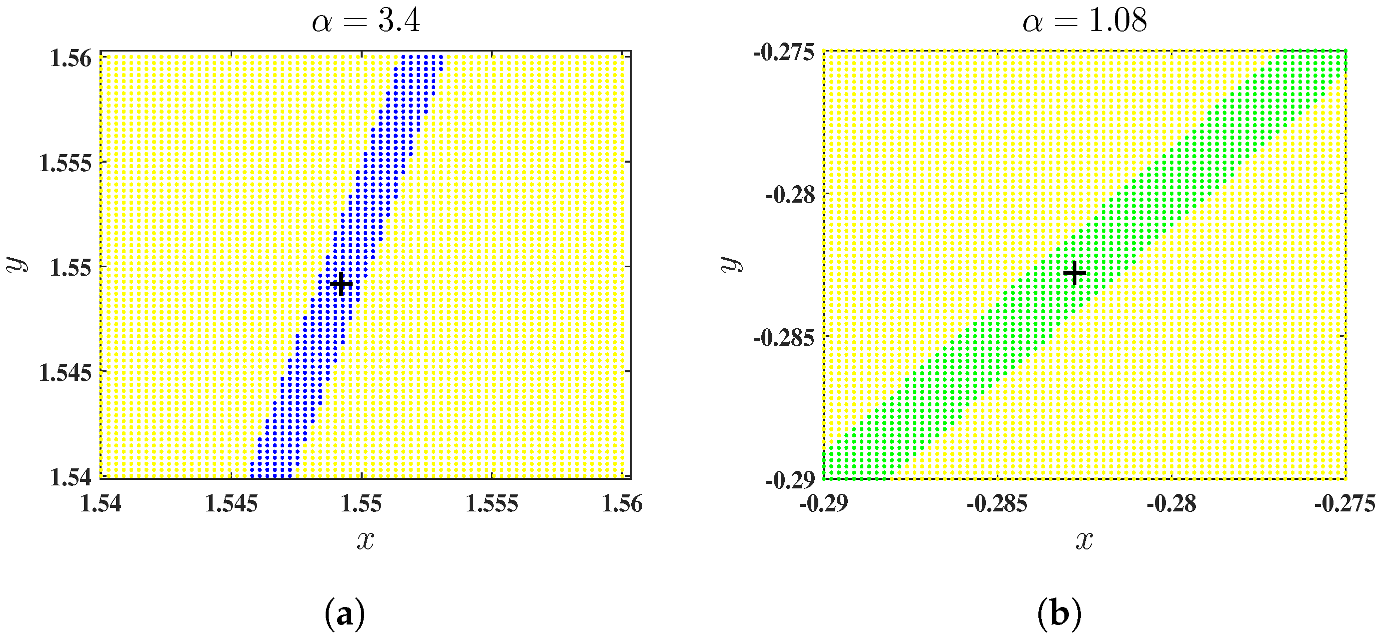
We numerically compute the value ${\delta }_{\epsilon }$ for a large number of values of $\alpha \in [1,5]$ for $\epsilon ={10}^{-8}$ and ${10}^{-6}.$ The results are presented in Figure 1. The equilibrium points where $|{\delta }_{\epsilon }|>\epsilon$ are plotted in blue; the equilibrium points where $|{\delta }_{\epsilon }|<\epsilon$ are plotted in green. In red, we label the points where $|{\delta }_{\epsilon }|-\epsilon$ change signs. It is remarkable that a small domain of attraction where the equilibrium points remain stable can always exist. As the value of $\epsilon$ increases, this domain shrinks, but it still exists around the equilibrium points. Therefore, the equilibrium points ${\underline{\tilde{x}}}_2$ and ${\underline{\tilde{x}}}_3$ are stable for $\alpha >1$.

Combining the results we have collected with the results in Section 4, we can draw the bifurcation diagram of System (13) (i.e., Equation (6)), as shown in Figure 2.

6. Numerical Results

6.1. General Solution

Example 1.

Let $x_{-1}=3$ and $x_0=-1$ be the initial conditions of Equation (6) where $\alpha =1.5$. Then, we use direct iteration of Equation (6) and we compare the results with the obtained explicit solution in Theorem 3. The results are shown in

Table 1. The values of $\left\{x_n\right\}$ for selected values of n for $\alpha =1.5$, $x_{-1}=3$, and $x_0=-1$.

n	Computed ${\mathit{x}}_{\mathit{n}}$ Using Equation (6)	Computed ${\mathit{x}}_{\mathit{n}}$ Using Formula (9)	Relative Error
1	$-2.250000000$	$-2.250000000$	0
2	$-0.461538461$	$-0.461538461$	0
3	$-1.655660378$	$-1.655660377$	$6.04\times {10}^{-10}$
4	$-0.392431098$	$-0.392431098$	$5.10\times {10}^{-10}$
5	$-1.505389744$	$-1.505389744$	0
6	$-0.370040735$	$-0.370040735$	$2.71\times {10}^{-10}$
7	$-1.450227418$	$-1.450227416$	$1.38\times {10}^{-9}$
8	$-0.361216641$	$-0.361216641$	$2.77\times {10}^{-10}$
9	$-1.427533184$	$-1.427533183$	$7.01\times {10}^{-10}$
10	$-0.357487158$	$-0.357487158$	$5.60\times {10}^{-10}$
350	$-0.354583236$	$-0.354583236$	$1.70\times {10}^{-9}$
477	$-1.410106147$	$-1.410106142$	$3.55\times {10}^{-9}$
500	$-0.354583236$	$-0.354583237$	$3.39\times {10}^{-9}$

. Table 1 sets forth the values of $\left\{x_n\right\}$ for selected values of n.

Example 2.

Let $x_{-1}=1.5$ and $x_0=2$ be the initial conditions of Equation (6) where $\alpha =0.25$. Then, Theorem 4 implies that the solution converges to zero.

Table 2. The values of $\left\{x_n\right\}$ for selected values of n for $\alpha =0.25$, $x_{-1}=1.5$, and $x_0=2$.

n	${\mathit{x}}_{\mathit{n}}$	n	${\mathit{x}}_{\mathit{n}}$
1	$9.375000000\times {10}^{-2}$	2	$4.210526316\times {10}^{-1}$
3	$2.254746836\times {10}^{-2}$	4	$1.042732222\times {10}^{-1}$
5	$5.623645354\times {10}^{-3}$	6	$2.605302816\times {10}^{-2}$
9	$3.514231287\times {10}^{-4}$	10	$1.628250901\times {10}^{-3}$
29	$3.351430075\times {10}^{-10}$	30	$1.552820828\times {10}^{-9}$

sets forth the values of $\left\{x_n\right\}$ for selected values of n. See also Figure 3.

Example 3.

Let $x_{-1}=-1$ and $x_0=2$ be the initial conditions of Equation (6) where $\alpha =-0.3$. Then, Theorem 4 implies that the solution converges to zero.

Table 3. The values of $\left\{x_n\right\}$ for selected values of n for $\alpha =-0.3$, $x_{-1}=-1$, and $x_0=2$.

n	${\mathit{x}}_{\mathit{n}}$	n	${\mathit{x}}_{\mathit{n}}$
1	$-0.3$	2	$-1.5$
3	$6.206896552\times {10}^{-2}$	4	$4.961977186\times {10}^{-1}$
5	$-1.806433560\times {10}^{-2}$	6	$-1.502056815\times {10}^{-1}$
9	$-1.620995677\times {10}^{-3}$	10	$-1.353048381\times {10}^{-2}$
29	$-9.571586670\times {10}^{-9}$	30	$-7.989673149\times {10}^{-8}$

sets forth the values of $\left\{x_n\right\}$ for selected small values of n. See also Figure 4.

6.2. Periodic Solutions

Example 4.

Using Theorem 7, we consider $\alpha =1.5$, $x_{-1}=0.75$, and $x_0=2/3$. Then, we obtain the periodic solution of period 2—see Figure 5.

Example 5.

Using Theorem 12, we consider $\alpha =-1$, $x_{-1}=0.5$, and $x_0=0$. Then, we obtain the periodic solution of period 4–see Figure 6.

6.3. Numerical Bifurcation Analysis

We perform a numerical bifurcation analysis for System (13). This analysis is based on a continuation method and uses the Matlab package MatContM—see [23,25,26]. Using $\underline{\tilde{x}}=(0,0),\alpha =0.1$, we continue the curve of the equilibrium point ${\underline{\tilde{x}}}_1$ with the free parameter $\alpha$. The NS bifurcation point is found along this curve. The computed NS point on this curve is given by ${\alpha }_{NS}=-1$. The normal form coefficient of the NS point computed by MatContM is 0. We obtained the same results in Section 4 (see Equation (23)). Further, we start again with a continuation with the free parameter $\alpha$ and using the initial data $\underline{\tilde{x}}=(2,2)$ and $\alpha =4$. We compute the curves of the equilibrium points ${\underline{\tilde{x}}}_2$ and ${\underline{\tilde{x}}}_3$. The branching point (BP), i.e., PF bifurcation, is computed along these curves and is given by ${\alpha }_{BP}=1$. The continuation leads to Figure 7.

It is remarkable that as we exceed the NS value ${\alpha }_{NS}$, a periodic solution of period 4 is born—see Figure 8. This is agreement with the results of Theorems 11 and 12.

6.4. The Basin of Attraction of the Equilibrium Points

To further corroborate the results in Section 5, we explore the basin of attraction of the equilibrium points ${\underline{\tilde{x}}}_2$ and ${\underline{\tilde{x}}}_3$ by performing ${10}^4$ map iterations for different initial points located in the ranges shown in Figure 9. We show the basins of attraction of the equilibrium points for five values of $\alpha$. In Figure 9, the points in the attraction domain of the equilibrium point ${\underline{\tilde{x}}}_1$ are colored red, the points in the attraction domain of the equilibrium point ${\underline{\tilde{x}}}_2$ are colored blue, and the points in the attraction domain of the equilibrium point ${\underline{\tilde{x}}}_3$ are colored green. The yellow points are these where no convergence was established after ${10}^4$ iterations. For $-1<\alpha <1$ (see Figure 9c,d), the basin of attraction of the equilibrium point ${\underline{\tilde{x}}}_1$ is connected, and then it shrinks and disappears as we leave this interval (see Figure 9e). It is clear that this is the case, since ${\underline{\tilde{x}}}_1$ is stable for $-1<\alpha <1$ and unstable otherwise. If $\alpha >1$, the basin of attraction of the equilibrium points ${\underline{\tilde{x}}}_2$ and ${\underline{\tilde{x}}}_3$ is very small and there are already points very close to the equilibrium points ${\underline{\tilde{x}}}_2$ and ${\underline{\tilde{x}}}_3$ that are not in its domain of attraction—see Figure 9a,b. However, numerical simulations show that the basin of attraction shrinks to the equilibrium points but never disappears at all. Therefore, these equilibrium points are, in fact, stable for $\alpha >1$.

7. Conclusions

We show that Equation (1) has exactly three equilibrium points. The trivial equilibrium point ${\tilde{x}}_1$ is globally asymptotically stable, while the equilibrium points ${\tilde{x}}_2$ and ${\tilde{x}}_3$ are never linearly stable. Using a nonlinear stability analysis criterion based on studying a small perturbation in the direction of the eigenvector corresponding to an eigenvalue equal to −1, we show that the equilibrium points ${\tilde{x}}_2$ and ${\tilde{x}}_3$ are stable (for $\alpha >1$) with a small domain of attraction. Additionally, we obtain an explicit formula for the general solution of Equation (1). 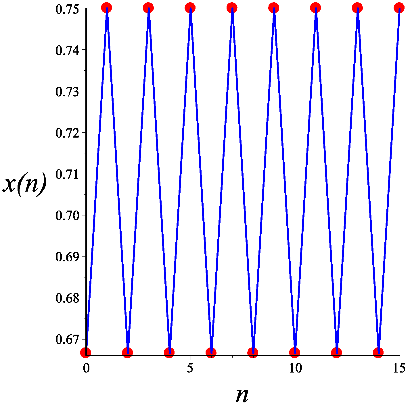We prove that if $(b/a)\in (-1,1)$, then every solution of Equation (1) converges to zero. We compute solutions of period 2 and 4 of Equation (1). Moreover, a complete bifurcation analysis is presented. We show that Equation (1) exhibits a Neimark–Sacker bifurcation. For the NS bifurcation, we compute the topological normal form. Finally, we perform a numerical simulation as well as a numerical bifurcation analysis using the Matlab package MatContM to confirm our theoretical results.