Abstract
Real-time pricing is an ideal pricing mechanism for regulating the balance of power supply and demand in smart grid. Considering the differences in electricity consumption risks among different types of users, a social welfare maximization model with user risk classification is proposed in this paper. Also, a smoothing Newton method is investigated for solving the proposed model. Firstly, the convexity of the model is discussed, which implies that the local optimum of the model is also the global optimum. Then, by transforming the proposed model into a smooth equation system based on the Karush–Kuhn–Tucker (KKT) conditions, we devise a smoothing Newton algorithm integrated with Powell–Wolfe line search criteria. The nonsingularity of the corresponding function’s Jacobian matrix is obtained to ensure the stability of the proposed algorithm. Finally, we give a comparison between the proposed model and the unclassified risk model and the proposed algorithm and the distributed algorithm for real-time pricing, time-of-use pricing, and fixed pricing, respectively. The numerical results demonstrate the effectiveness of the model and the algorithm.
Keywords:
smart grid; complementarity problems; KKT conditions; smoothing Newton algorithm; nonsingularity; classification of electricity risks; multiple prices MSC:
90C90
1. Introduction
With the rapid development of the social economy, the demand for electricity in various industries is increasing. However, the serious shortage of electric power energy and the low efficiency of complementary and coordinated dispatching in multi-energy power systems have already become major obstacles that restrict the economic development of countries around the world. Strengthening the construction of new power systems and improving the complementary and coordinated dispatching of multi-energy power systems are important and urgent.
In recent years, smart grids have emerged as a core focus of the global energy transition due to their high energy efficiency, enhanced grid stability, and improved reliability. Within this evolution, the large-scale integration of renewable energy and the innovative implementation of real-time pricing mechanisms, which are important means of demand-side management and aim to adjust the balance of electricity supply and demand [1,2,3,4], have become pivotal. As the proportion of intermittent renewable energy sources, such as wind and solar power, continues to rise, smart grids leverage advanced data sensing and predictive technologies to dynamically optimize energy dispatch strategies, effectively mitigating the impact of renewable energy fluctuations on grid stability. Simultaneously, real-time pricing mechanisms based on supply–demand dynamics not only incentivize users to shift consumption away from peak periods—enhancing load flexibility—but also drive intelligent responses from energy storage systems and distributed energy resources through price signals. This fosters a coordinated “source–grid–load–storage” energy ecosystem. The deep integration of these two innovative elements not only improves the absorption capacity for clean energy but also achieves spatiotemporal optimization of power resource allocation through market-driven approaches, delivering dual drivers for building a low-carbon, resilient, and highly efficient modern energy system.
Actually, renewable energy sources have received extensive attention in this decade [5,6,7,8,9], and have become an important part of the new power system due to their low development costs, and being clean and pollution-free. However, the output power of distributed power sources may be affected by various conditions, such as light intensity, temperature, fan radius, and the windward angle of the blades. The input of high-proportion renewable energy into the smart grid may lead to unstable power output, resulting in uncertainties in the power supply system of the smart grid and power supply risks. In the last decade, some researchers have considered some risks and uncertain factors in power grids [10,11,12,13,14,15,16,17,18]. Tarasak et al. proposed three cases of uncertain electricity consumption, namely boundary uncertainty, Gaussian distribution, and unknown distribution, and then concluded that uncertain electricity consumption would lead to an increase in electricity prices [10]. Wang et al. [11] adopted variance as a risk assessment measure and subtracted a risk term for electricity fluctuations from the objective function in the model proposed by Samadi. Tang and Yang et al. proposed a heuristic dynamic pricing algorithm to identify handle users and unstable power suppliers [12]. Zhu et al. considered the risks brought by the fluctuation in total electricity demand to power suppliers, and introduced risk factors into the model to improve the effectiveness and rationality of the real-time pricing strategy [13]. A new two-level real-time pricing model was proposed in Ref. [14], where different distributed energy sources, the uncertainty of renewable energy generation, carbon trading mechanisms, and grid fluctuations are considered. These studies have played important role in the progress of constructing the new power grid. However, this existing research is mostly based on the electricity risk for single users, seen in Refs. [11,14], uncertain models based on the classification of electrical appliances, seen in Ref. [12], or unstable power suppliers, seen in [13,15]; a model based on user risk classification is rarely mentioned, which may lead to the fluctuations in overall social electricity consumption, resulting in the transition between the peak and the valley.
Real-time pricing is becoming an important direction in the smart grid pricing mechanism. Considering that the dynamic changes in the total electricity demand of users may bring risks to the smart grid even when the power generation is stable, such as causing unnecessary waste when the total electricity demand of users is lower than the generated electricity, resulting in power outages and requiring emergency measures when the total demand for electricity exceeds the generated capacity, it is necessary to consider the fluctuation risk of total electricity demand of users in the real-time pricing mechanism. Inspired by Ref. [13], a model based on user risk classification for real-time pricing is proposed in this paper. Also, a smoothing Newton method with global convergence and local quadratic convergence is investigated for solving the proposed method. Compared with the existing literature, the contributions of this paper are as follows: (1) A nonlinear optimization model is proposed to maximize social welfare based on user risk classification; namely, the electricity consumption risks of residential users and commercial users are considered separately. (2) A smoothing Newton method with Powell–Wolfe line search criteria is investigated based on (KKT) conditions, which could overcome the small step size in the Armijo search method. (3) We prove the nonsingularity of the Jacobian matrix, and then the global convergence and local quadratic convergence of the smoothing Newton algorithm are obtained. (4) We give a comparison between the proposed model and the unclassified risk model and the proposed algorithm and the distribute algorithm for real-time pricing, time-of-use pricing, and fixed pricing, respectively. The numerical results show that the price obtained is lower, and the total welfare is higher, which implies the effectiveness of the model and algorithm. Furthermore, we consider the electricity consumption rise for different users, and the results could help the electricity supply optimize resource allocation according to user types. And by guiding users to consume electricity rationally, the government could guide users use electricity rationally, such as reduce power consumption during peak electricity load periods and increase power consumption during low load periods, so as to achieve the effect of peak shaving and valley filling.
The outline of this paper is organized as follows. In Section 2, some related models for the real-time pricing problem in smart grids are introduced. In Section 3, model user risk classification is established and its equivalent equation is obtained. In Section 4, a smoothing Newton algorithm is proposed, and its convergence is obtained by proving the nonsingularity of the Jacobian matrix. In Section 5, simulation experiments are given to illustrate the reasonableness of the proposed model and the effectiveness of the proposed algorithm.
2. System Model
In this section, we give the model based on user electricity consumption classification.
In a smart grid system that includes a power provider and multiple users, each user is equipped with an electrical consumption controller, ECC for short, which is used to control the electricity consumption of users and exchange real-time information with each other.
Since each user is an independent individual in the smart grid, the demand can be characterized by different parameters, such as different times of day, climate conditions, electricity prices, and other factors. And it also depends on the type of the users. For residential and commercial users with the same electricity price, there will be different reactions, which can be characterized by the utility functions in microeconomics. These functions represent the relationship between consumption utility and quantity of goods. Denote as the utility functions. They are usually increasing concave functions and satisfy the following properties.
(1) An increasing function: ,
(2) Marginal decline function: .
Consider a smart grid system that includes a power supplier and multiple users. Divide the whole cycle into K periods and let N be the set of users requiring electricity, be the power consumption demand at the slot of the i-th users, and be the total generation capacity at the slot k. Samadi et al. [19,20] proposed a model called the social welfare maximization model (SWMM) to maximize the aggregated welfare for the users and power supplies as follows.
where the constraint conditions mean that the electricity consumption of all users does not exceed the total generating capacity, and is the cost function of the power supply.
Considering the impact of the uncertainty of user electricity demand on real-time electricity prices when the power generation remains relatively stable, the mean variance term of electricity load is added in the SWMM model and an online real-time electricity price risk model is proposed in Ref. [11]. It is such that
where , and . However, the fluctuations in individual user electricity consumption may not cause fluctuations in the total social electricity consumption in the real power system; the online real-time electricity price risk model may exaggerate the risk of electricity consumption fluctuations to some extent, and it may make the social welfare function smaller. Then, Zhu proposed a real-time electricity pricing model based on the overall electricity risk of users in Ref. [13], where the variance is modified into a form such that
here represents the total user power consumption at time k, and
Actually, different types of users have distinct electricity consumption behaviors, demands, and risk tolerance capabilities. The electricity consumption of residential users mainly focuses on daily life scenarios, such as lighting, cooking, and the use of household appliances. In contrast, commercial users, especially large industrial enterprises, have a large electricity consumption scale and heavy load, and they have extremely high requirements for the stability of electricity supply during the production process. Establishing and solving a model based on users’ electricity consumption differences and risks can effectively balance the interests of all parties and achieve the optimal allocation of electricity resources.
Suppose a power system consists of a single energy supplier, residential load users, and commercial users. and represent the power consumption requirements of residential users and commercial users in time slot k, respectively. Inspired by Ref. [13], and combining the difference in electricity consumption for different users, we adopt different risk factors to reconstruct the single-user online real-time risk model into an online real-time risk model for classified users, and proposed a real-time pricing model based on user risk classification in this paper. It is such that
where , , , , and
In this model, users are divided into two types. The electricity consumption risk of each user is related to the electricity consumption risk coefficient and the electricity consumption amount at the previous moment. Table 1 summarizes the differences between the existing literature and the proposed models.

Table 1.
Existing research comparison.
Remark 1.
Model (1) is a convex optimization problem. Set where and By straight calculation, one obtains Therefore, and are convex functions. The utility function , which is concave, is combined, and the cost function is always adopted as a quadratic function such that
so model (1) is actually a convex problem.
3. Model Transformation
In optimization theory, the Karush–Kuhn–Tucker (KKT) condition is a necessary condition for the optimal solution of nonlinear programming. In this section, the model transformation is given based on the KKT condition.
The KKT condition was independently published by Karush in 1939 and by Kuhn and in 1951; it is both a necessary condition and a sufficient condition for convex programming. Consider an inequality-constrained optimization problem such that
If is its extreme point, and exist and the KKT conditions is as follows.
Consider the time slot k of model (1); it is a optimization problem such that
and we next give its transformation based on the KKT condition.
Denote
and
where , .
If is its extreme point, then exists and KKT can be established under the conditions that
Furthermore, since
is a complementarity problem, the equivalent nonsmooth system of model (2) is as follows.
where is an “NCP” function, such as the minimum function , the Fischer–Burmeister function , and so on [21,22,23]. The system of Equation (3) is nonsmooth. Since it is difficult or time-consuming to obtain the generalized differential for a Lipschitzian function, we consider the smoothing algorithm and adopt the function
based on which, the equivalent smooth equation system model of (3) is obtained as follows.
where and
Actually, the system of Equation (4) is equivalent to model (3), since it is obvious that
4. Algorithm and Convergence
In this section, we use a smoothing Newton algorithm to solve Equation (4) and give its convergence by proving the nonsingularity of the relate function’s Jacobian matrix.
First, let . We introduce the smoothing Newton algorithm as follows (Algorithm 1).
| Algorithm 1: Smoothing Newton algorithm |
|
Remark 2.
Step 3 in Algorithm 1 is the Powell–Wolfe search method, which could overcome the small step size in the Armijo search method. Actually, the step size will not be too large or too small, and is bounded.
Remark 3.
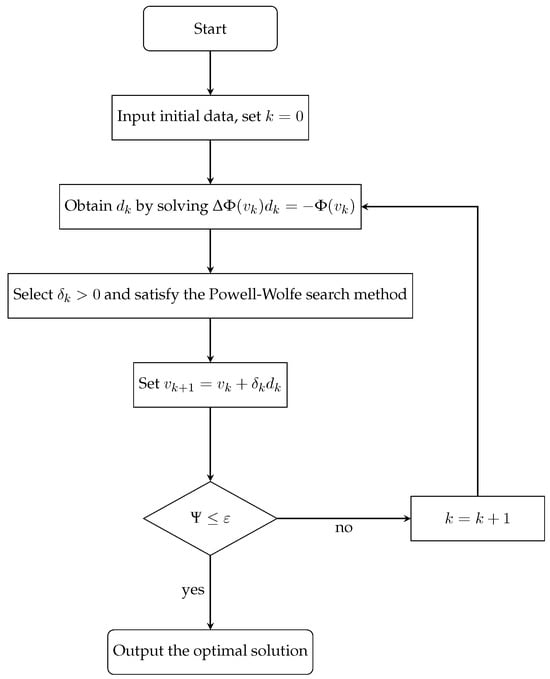
During the operation of Algorithm 1, it is necessary to calculate the gradient of the smoothing function at each time, which usually takes time. In terms of space complexity, the algorithm needs to store the gradient, intermediate variables in the iterative process, and so on; the space complexity is (Figure 1).
Figure 1.
Comparison The flow chart of Algorithm 1.
Remark 4.
The smoothing Newton algorithm is an effective one for solving nonsmooth systems of equations. The nonsingularity of the Jacobian matrix is crucial in the algorithm. If the matrix is singular, it will lead to difficulties in solving the linear equation system, making it impossible to obtain an accurate search direction. Consequently, the convergence of the algorithm will be disrupted, and in severe cases, divergence may occur, significantly affecting the stability and effectiveness of the algorithm. Only when the Jacobian matrix is nonsingular can the algorithm update iteratively based on reliable information, approach the optimal solution, and effectively handle nonsmooth problems. We next discuss the nonsingularity of .
Actually, by straight calculation, the expression of the Jacobian matrix of is such that
where
and
Set
and there is
Obviously, is nonsingular if and only if is nonsingular. Actually, by elementary transformation, the matrix J can be transformed into the ladder matrix such that
where .
When , , . For , the recurrence formula can be expressed as follows: , . The final result can be expressed as follows: , .
We next investigate the determinant of and conclude Theorem 1 as follows.
Theorem 1.
The Jacobian matrix of is nonsingular.
Proof of Theorem 1.
Consider the determinant of . Since , , , and the risk factors , , it is obvious that if , , , one obtains ; namely, J is nonsingular.
Since , , , and , and are the i-th and j-th users’ optimal consumption quantity, and and are the optimal power generation. In fact, the optimal power generation is the sum of users’ electricity consumption; for k large enough, one has and . Thus, the recurrence formulas of and are all calculations of addition, multiplication, and division between positive numbers, and, obviously, and .
For q, one has
Furthermore, since , one obtains
For q, similar to the proof of p, one has
Then, combining it with , the conclusion holds. □
Actually, the algorithm has global convergence. We give the global and local convergent result as follows.
Lemma 1.
Suppose is generated by Algorithm 1; is monotonically decreasing and bounded.
Proof of Lemma 1.
which implies is monotonically decreasing, namely, , and it is bounded. □
The conclusion is obvious. Firstly, since , by virtue of step 3 in Algorithm 1, one obtains
Remark 5.
By virtue of Theorem 1 and Lemma 1, Algorithm 1 is well posed. Actually, Equation (5) has a unique solution, which means that step 2 is well posed. Then, from Theorem 2.2.2 in reference [24], it is found that if has a lower bound with respect to , then there exists a that satisfies the Powell–Wolfe step length criterion.
Theorem 2.
(Global convergence) Suppose is generated by Algorithm 1, and is an accumulation point of the sequence generated by Algorithm 1; then, .
Proof of Theorem 2.
By virtue of Lemma 1, one obtains
Since , one has
Then,
Furthermore, considering that
one has
Then, one obtains
which contradicts , and the conclusion holds. □
We divide the proof into two parts.
(i) Firstly, we prove that the sequence has at least one accumulation point. Obviously, is smooth here, since is convergent, and there must exist such that , which implies that the sequence has least one accumulation point. Without loss of generality, denote as the subsequence of such that .
(ii) We next prove by contradiction. Suppose ; then, for a sufficiently large t, there exists no , satisfying the conditions that
namely, there exists such that
Similar to the proof of Theorem 1 in Ref. [25], the quadratic convergence of Algorithm 1 is obvious since is Lipschitz-continuous; we give the conclusion, namely Theorem 3 as follows, and omit its proof.
Theorem 3.
(Local convergence) Suppose is generated by Algorithm 1, is Lipschitz-continuous, and is an accumulation point of the sequence ; then, .
5. Numerical Experiments
In this section, we present some numerical simulations to illustrate the performance of the model and the proposed algorithm. Firstly, we give a comparison of the real-time pricing and the welfare between the classified risk model and the unclassified risk model based on different user scales. Then, the proposed algorithm is compared with the distributed algorithm and one-step Levenberg–Marquardt method based on the risk-classified model, respectively. Also, we investigate the effectiveness of the proposed algorithm for different electricity pricing mechanisms, such as real-time pricing, time-of-use pricing, and fixed electricity pricing. The Dell computer, manufactured by Dell Inc. in Round Rock, TX, USA, is equipped with an 11th Gen Intel(R) Core(TM) i5-11320H, and we coded the algorithm in Matlab R2018A.
Considering the smart grid system in a small area, we present numerical simulation results within a 24 h time pattern as an evaluation of daily operations. The electricity demand of residential users was randomly selected from , with . The electricity demand of commercial users was randomly selected from , with . In the utility function, and , using and in the cost function, and the initial price and . Meanwhile, the initial power supply and ; we adopted , , , , , and .
5.1. Risk-Classified Real-Time Pricing Model and Risk-Unclassified Real-Time Pricing Model Based on the Smoothing Newton Algorithm
In the risk-classified real-time pricing model (i.e., (2)), users are divided into residential groups and commercial groups, and each group is assigned a different risk factor. In the risk-unclassified real-time pricing model (i.e., (1)), all users form a separate group and are supplied with electricity based on a single risk factor. Here, we use the proposed algorithm to solve the risk-classified model and the risk-unclassified model, respectively. In addition, we choose different numbers of resident users and commercial users. We set , , and . The comparison of the price and the social welfare results are shown in Figure 2 and Figure 3.
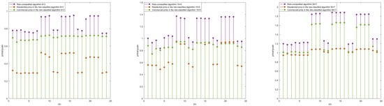
Figure 2.
Comparison of price between the risk-classified model and unclassified model under different scales of users based on the smoothing Newton algorithm.
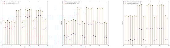
Figure 3.
Comparison of the social welfare between risk-classified model and unclassified model under different scales of users based on the smoothing Newton algorithm.
As shown in Figure 2, the price in the risk-classified algorithm is lower than that in the risk-unclassified algorithm. As shown in Figure 3, the social welfare in the risk-classified algorithm is higher than that in the risk-unclassified algorithm, which indicates that the classification model algorithm is more effective in calculating the electricity prices and the welfare, even for different numbers of resident users and commercial users. In the case of the non-classification model, it fails to take into account the diversified consumption characteristics and needs of different residential users, resulting in overestimated electricity prices. In contrast, the classification model algorithm, by categorizing users based on various factors such as consumption patterns and load characteristics, can better allocate costs and provide more reasonable real-time electricity prices. This distinction not only has implications for users in terms of cost savings but also plays a crucial role in promoting the efficient operation and management of the power grid system.
In addition, the risk-classified algorithm takes into account the conditions and characteristics of different user types, making it more reasonable than the risk-unclassified algorithm. The risk-classified model has a greater total social welfare than the risk-unclassified model, which further illustrates that the conditions and characteristics of different user types are more reasonable than a single risk factor, and also indirectly illustrates the effectiveness of model (2).
5.2. Comparison of the Smoothing Newton Algorithm and Distributed Algorithm
In this section, we compare the proposed algorithm with the distributed algorithm in Ref. [26] to solve the residential electricity price, the commercial electricity price, and the total social welfare of the risk-classified model, and the results are shown in Figure 4.
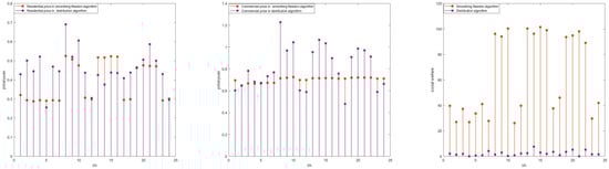
Figure 4.
Comparison of price and the social welfare between the smoothing Newton algorithm and the distributed algorithm.
As shown in Figure 4, the electricity prices for residential and commercial users under the smoothing Newton algorithm are generally lower than those under the distributed algorithm. As is evident from the figures, the electricity prices obtained through the smoothing algorithm are generally lower than those derived from the distributed algorithm. This price disparity has a direct and significant impact on social welfare. The lower electricity prices generated by the smoothing algorithm mean that consumers, whether they are households or enterprises, can enjoy reduced electricity costs, which could free up more financial resources for them to allocate to other aspects of consumption or production, thereby stimulating economic activities and promoting overall social development.
Actually, we also compare the proposed algorithm with the one-step Levenberg–Marquardt method [27], which is proposed for nonlinear equations. However, it always takes much more time to obtain the result. We omit the result here.
5.3. Comparison of the Real-Time Pricing (RTP) with Time-Of-Use Pricing (TOU) and Fixed Pricing (FP)
In this section, we analyze the performance of the proposed algorithm under three different pricing mechanisms: RTP, TOU and FP.
Time-of-use pricing divides a day into multiple periods, such as peak and off-peak periods, and sets different electricity prices for each period to guide users in adjusting their electricity consumption behavior. Fixed pricing, on the other hand, maintains a constant price per unit of electricity regardless of when the user consumes it. We calculate the electricity prices for residential and commercial users under these three pricing mechanisms, as well as the corresponding social welfare. Inspired by Ref. [28], the electricity demand characteristics of different user groups are fully considered, and different price equations are selected. For residential users, we have the following: , , and , which are the FP, peak price, and trough price of TOU, respectively. In the same way, for commercial users, we know that , , and , which are the FP, peak price, and trough price of TOU, respectively. Here, we set and as the largest satisfactory parameters for resident users and commercial users, respectively. , , and are the maximum power consumption, minimum power consumption, and average power consumption of during the period k, respectively, and . The other constant parameters are set as follows: and .
Based on the price formulas above and the corresponding parameters, the results of the RTP, TOU, and FP strategies are shown in Figure 5.
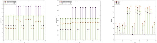
Figure 5.
Comparison of price and the social welfare between the RTP, TOU, and FP strategies.
From Figure 5, the electricity prices under the real-time pricing mechanism fluctuate most frequently, responding promptly to changes in supply and demand in the power grid. During peak electricity consumption periods, prices rise significantly, effectively curbing excessive demand, while during off-peak periods, prices decrease accordingly, encouraging users to increase consumption. The time-of-use pricing mechanism also shows distinct period-based price differences, with higher prices during peak periods and lower prices during off-peak periods; however, the price adjustment is singular compared with real-time prices. Under the fixed pricing mechanism, electricity prices remain stable and do not change with time or supply and demand variations. In addition, it is obvious that the social welfare of the RTP method is higher than that of the TOU and FP mechanisms, which shows that the RTP method has better performance than the TOU and FP mechanisms in improving social welfare.
6. Conclusions
In this paper, we proposed a real-time pricing model for smart grids based on user risk classification, and correspondingly constructed a smoothed Newton algorithm. By proving the nonsingularity of the Jacobian matrix, the implementation of the algorithm is guaranteed, and the results of numerical experiments showed the effectiveness of the model and the proposed algorithm. The proposed model is more in line with reality. Numerical results show that the electricity price is lower, and the social welfare is higher. During peak electricity consumption periods, the algorithm outputs relatively higher electricity prices, and the government could encourage users to reduce their electricity demand from an economic perspective, thereby achieving peak shaving. Conversely, during off-peak periods, the government could provide lower electricity prices to incentivise users to increasing their electricity usage. Therefore, further application of this model can be considered in practical problems. However, the Newton algorithm has certain limitations. It is necessary to calculate the Jacobian matrix in each iteration. And the calculation scale in this paper is also relatively small, so it is necessary to find an approximate form, which could replace the calculation of the Jacobian matrix for larger-scale power grid systems. In addition, the choice of the parameters is similar to the related reference. During the operation of the algorithm, conducting an analysis of the sensitivity in the proposed model would be a very meaningful and important task, which is our next topic.
Author Contributions
Conceptualization, L.S.; methodology, L.S.; software, G.S.; validation, L.S. and G.S.; formal analysis, G.S.; resources, L.S.; data curation, G.S.; writing—original draft preparation, G.S.; writing—review and editing, L.S.; supervision, L.S.; project administration, L.S.; funding acquisition, L.S. All authors have read and agreed to the published version of the manuscript.
Funding
This work was supported by the National Science Foundation of China (no.12101198) and Henan Province science and technology research project (no.242102210057).
Data Availability Statement
The data are contained within the article.
Conflicts of Interest
The authors declare no conflicts of interest.
Abbreviations
The following abbreviations are used in this manuscript:
| KKT | Karush-Kuhn-Tucker |
| SWMM | Social welfare maximization model |
| NCP | Nonlinear complementarity problem |
| RTP | Real-Time Pricing |
| TOU | Time-of-Use Pricing |
| FP | Fixed Pricing |
References
- Ghole, M.S.; Paliwal, P.; Thakur, T. Sensitivity analysis of priority-based demand response metrics with continuous real-time pricing scheme using swap-based butterfly particle swarm optimization. Arab. J. Sci. Eng. 2024, 49, 6923–6940. [Google Scholar] [CrossRef]
- Tang, D.G.; Guerrero, J.M.; Zio, E. Securing demand-response in smart grids against false pricing attacks. Energy Rep. 2024, 12, 892–905. [Google Scholar] [CrossRef]
- Ma, K.; Kang, C.; Liu, P.; Yuan, Y.; Yang, J.; Li, H. Demand-Side Relay Spectrum Allocation in Smart Grid Based on Bilateral Auction. IEEE Trans. Ind. Inform. 2024, 20, 12717–12725. [Google Scholar] [CrossRef]
- Tepe, I.F.; Irmak, E. Optimizing real-time demand response in smart homes through fuzzy-based energy management and control system. Electr. Eng. 2024, 107, 2121–2145. [Google Scholar] [CrossRef]
- Yang, M.; Li, X.; Fn, F.; Wang, B.; Su, X.; Ma, C. Two-stage day-ahead multi-step prediction of wind power considering time-series information interaction. Energy 2024, 312, 133580. [Google Scholar] [CrossRef]
- Yang, M.; Che, R.; Yu, X.; Su, X. Dual NWP wind speed correction based on trend fusion and fluctuation clustering and its application in short-term wind power prediction. Energy 2024, 302, 131802. [Google Scholar] [CrossRef]
- Li, N.; Dong, J.; Liu, L.; Li, H.; Yan, J. A novel EMD and causal convolutional network integrated with Transformer for ultra short-term wind power forecasting. Int. J. Electr. Power Energy Syst. 2023, 154, 109470. [Google Scholar] [CrossRef]
- Deng, X.T.; Zhang, Y.; Jiang, Y.; Qi, H. A novel operation method for renewable building by combining distributed DC energy system and deep reinforcement learning. Appl. Energy 2024, 353, 122188. [Google Scholar] [CrossRef]
- Li, P.; Hu, J.; Qiu, L.; Zhao, Y.; Ghosh, B.K. A distributed economic dispatch strategy for Power–Water networks. IEEE Trans. Control Netw. Syst. 2022, 9, 356–366. [Google Scholar] [CrossRef]
- Tarasak, P. Optimal real-time pricing under load uncertainty based on utility maximization for smart grid. In Proceedings of the 2011 IEEE International Conference on Smart Grid Communications, Brussels, Belgium, 17–20 October 2011; pp. 321–326. [Google Scholar]
- Wang, Y.; Mao, S.W.; Nelms, R.M. Distributed online algorithm for optimal real-time energy distribution in the smart grid. IEEE Internet Things J. 2014, 1, 70–80. [Google Scholar] [CrossRef]
- Tang, Q.; Yang, K.; Zhou, D.; Luo, Y.; Yu, F. A real-time dynamic pricing algorithm for smart grid with unstable energy providers and malicious users. IEEE Internet Things J. 2016, 3, 554–562. [Google Scholar] [CrossRef]
- Zhu, H.B.; Gao, Y.; Dai, Y.M. Real-time pricing strategy considering the risk of smart grid. J. Syst. Simul. 2019, 30, 1376–1383. [Google Scholar]
- Wang, J.Q.; Gao, Y.; Li, R.J. Reinforcement learning based bilevel real-time pricing strategy for a smart grid with distributed energy resources. Appl. Soft Comput. 2024, 155, 111474. [Google Scholar] [CrossRef]
- Cao, W.L.; Zhou, L. Resilient microgrid modeling in Digital Twin considering demand response and landscape design of renewable energy. Sustain. Energy Technol. Assess. 2024, 64, 103628. [Google Scholar] [CrossRef]
- Yuan, G.X.; Gao, Y.; Ye, B.; Huang, R. Real-time pricing for smart grid with multi-energy microgrids and uncertain loads: A bilevel programming method. Int. J. Electr. Power Energy Syst. 2020, 123, 106206. [Google Scholar] [CrossRef]
- Cui, G.; Jia, Q.S.; Guan, X. Energy management of networked microgrids with real-time pricing by reinforcement learning. IEEE Trans. Smart Grid 2024, 15, 570. [Google Scholar] [CrossRef]
- Tao, L.; Gao, Y.; Liu, Y.; Zhu, H. A rolling penalty function algorithm of real-time pricing for smart microgrids based on bilevel programming. Eng. Optim. 2020, 52, 1295–1312. [Google Scholar] [CrossRef]
- Samadi, P.; Mohsenian-Rad, A.H.; Schober, R.; Wong, V.W.; Jatskevich, J. Optimal real-time pricing algorithm based on utility maximization for smart grid. In Proceedings of the 2010 First IEEE International Conference on Smart Grid Communications, Gaithersburg, MD, USA, 4 October 2010; pp. 415–420. [Google Scholar]
- Asadi, G.; Gitizadeh, M.; Roosta, A. Welfare maximization under real-time pricing in smart grid using PSO algorithm. In Proceedings of the 2013 21st Iranian Conference on Electrical Engineering (ICEE), Mashhad, Iran, 14–16 May 2013; pp. 1–7. [Google Scholar]
- Cottle, R.W.; Pang, J.; Stone, R. The Linear Complementarity Problem; Academic Press: Boston, MA, USA, 1992. [Google Scholar]
- Fischer, A. A special Newton-type optimization method. Optimization 1992, 24, 269–284. [Google Scholar] [CrossRef]
- Chen, J.S.; Huang, Z.H.; She, C.Y. A new class of penalized NCP-functions and its properties. Comput. Optim. Appl. 2011, 50, 49–73. [Google Scholar] [CrossRef]
- Wang, Y.J.; Xiu, N.H. Nonlinear Optimization Theory and Methods, 3rd ed.; Science Press: Beijing, China, 2019. [Google Scholar]
- Ma, C.F.; Wang, T. The smoothing Newton method fro NCP with P0-mapping based on a new smoothing function. Math. Appl. 2023, 36, 589–601. [Google Scholar]
- Xu, Z.H.; Guo, L.Y.; Gao, Y. Real-time pricing of smart grid based on piece-wise linear functions. J. Syst. Sci. Inf. 2019, 7, 295–316. [Google Scholar] [CrossRef]
- Yu, H.D.; Pu, D.G. Smoothing Levenberg-Marquardt method for general nonlinear complementarity problems under local error bound. Appl. Math. Model. 2011, 35, 1337–1348. [Google Scholar] [CrossRef]
- Li, Y.Y.; Li, J.X.; Yu, Z.S.; Dong, J.; Zhou, T. A cosh-based smoothing Newton algorithm for the real-time pricing problem in smart grid. Electr. Power Energy Syst. 2022, 135, 107296. [Google Scholar] [CrossRef]
Disclaimer/Publisher’s Note: The statements, opinions and data contained in all publications are solely those of the individual author(s) and contributor(s) and not of MDPI and/or the editor(s). MDPI and/or the editor(s) disclaim responsibility for any injury to people or property resulting from any ideas, methods, instructions or products referred to in the content. |
© 2025 by the authors. Licensee MDPI, Basel, Switzerland. This article is an open access article distributed under the terms and conditions of the Creative Commons Attribution (CC BY) license (https://creativecommons.org/licenses/by/4.0/).