Coverage Optimization with Balanced Capacitated Fragmentation

Abstract

This paper investigates a specialized variant of the set covering problem, addressing the optimal allocation of service centers to ensure that all customers (or larger entities, such as urban areas) have access to specialized services within a predefined acceptable distance, referred to as the threshold. In addition to minimizing the number of service centers required or their total cost, this study emphasizes the critical importance of balancing capacity fragmentation—defined as the uneven distribution of service demand across facilities—to enhance accessibility and ensure equitable service delivery for customers. We propose an innovative mathematical model with additional practical constraints related to service deployment and designed to optimize both coverage and capacity fragmentation within a defined region. The model is validated through simulations implemented in GAMS, which document that this software tool is capable of solving even large problem instances in a reasonable amount of time. The results demonstrate the model’s effectiveness in addressing real-world challenges associated with equitable and efficient service allocation.

1. Introduction

The optimization of the placement and operation of public facilities, such as hospitals and schools, has been an area of significant focus in recent years [1,2,3]. These facilities provide essential services, including healthcare and education, to the population, and their efficient allocation is crucial to ensuring both accessibility and cost effectiveness. The primary objective is to design a network in which each inhabitant or urban district has access to at least one service center within a reasonable distance, while minimizing operational costs.

A key issue in this optimization process is determining what constitutes an “affordable” or “reasonable” distance for accessing these facilities. This determination is often subjective and can vary based on local contexts, geographical constraints, and political priorities. Governments and political parties often set these thresholds to align with social equity goals or regional development strategies. However, for the purpose of this study, we set aside the political and sociological dimensions of the problem and focus exclusively on its mathematical and computational aspects.

In mathematical terms, such problems are frequently addressed using optimization techniques that aim to ensure the full coverage of a population while adhering to specific constraints, such as distance limits. A widely studied model in this context is the set covering problem. This problem seeks to identify the smallest subset of facilities necessary to cover all demand points as specified by a binary reachability matrix. Notably, the traditional set covering problem does not account for specific thresholds for availability or accessibility but, instead, relies on a predefined binary matrix to indicate whether a demand point is within reach of a given facility.

The set covering problem is classified as NP-hard [4,5], meaning that as the problem size increases, the computational complexity grows exponentially, rendering exact solutions impractical for large-scale instances. Consequently, heuristic methods are often employed to generate approximate solutions within a reasonable timeframe. These methods aim to strike a balance between computational efficiency and solution quality, making them suitable for real-world applications where time and resources are limited.

The problem we address in this paper is closely related to the general set covering problem. By introducing a threshold for acceptable distances between facilities and demand points, we transform the distance matrix into a binary reachability matrix, where entries indicate whether a facility can serve a particular demand point within the threshold distance. This conversion allows us to formulate and solve the problem as a set covering problem, utilizing well-established mathematical models and solution techniques to address the underlying optimization challenge. However, as highlighted in the literature review (Related Work section),  the existing models, while primarily focusing on coverage and capacity constraints, often neglect the challenge of capacity fragmentation—the imbalance in demand distribution across facilities—which can lead to inequitable and inefficient service allocation. Traditional models such as CLSCP-CA, CLSCP-EA, and CLSCP-SO have made notable advancements in capacity-based location problems, but they fall short in addressing the simultaneous optimization of both coverage and balanced capacity fragmentation. This research addresses this gap by proposing a novel model that explicitly incorporates capacity fragmentation considerations into the set covering framework, advancing the field beyond the existing approaches.

1.1. Main Contribution

In this paper, we introduce an innovative mathematical model designed to address the unique challenges of location covering problems with balanced fragmented capacity allocation. The model focuses on the efficient distribution of service capacities and the fragmentation of demand across multiple service centers, ensuring that no facility is overburdened while fully meeting the customer demand. This approach is particularly valuable for scenarios such as the deployment of new service centers in underserved regions, optimizing the use of existing facilities, or consolidating infrastructure between different providers. Our main contribution consists in the development of a model that incorporates both direct and optional capacity assignments, while adhering to the critical constraints of overlapping service areas and ensuring that only selected centers fulfill the demand. We validate the model’s effectiveness through simulations using the General Algebraic Modeling System (GAMS) tool, which allows for easy rewriting of the model into source code and, thanks to built-in heuristics, also for finding the optimal solution in a reasonable time even for large instances of problems with exponential complexity, in the studied case with complexity $\mathcal{O}\left(2^n\right)$. The simulation results highlight the model’s ability to handle complex demands and optimize resource distribution in practical settings.

1.2. Paper Organization

This paper is organized into six sections. Section 1 provides an overview of the problem and the context in which it arises. Section 2 presents the formal problem formulations underlying the study, including the key optimization challenges. Furthermore, this section covers the literature review and its gaps. Section 3 introduces the newly developed mathematical model for area coverage capacity problems, explaining its key components and contributions to the field. Section 4 discusses the complexity of the problem and the methods used for its implementation aspects. Section 5 presents simulation results that validate the model’s effectiveness in real-world scenarios, followed by an analysis of the outcomes. Finally, Section 6 concludes the paper, summarizing the main findings and conclusions.

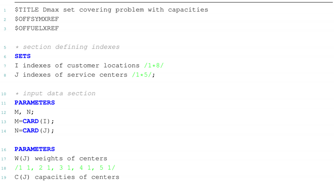
2. Problem Formulations

Assume a transport network consisting of m vertices to be served and n vertices that can potentially function as operating service centers. For each pair of vertices, $v_i$ (regarded as a customer location or serviced vertex) and $v_j$ (service center), their distance $d_{ij}$ is given, with $D_{max}$ representing the maximum allowable distance between the serviced vertices and service centers.

Let I and J denote two finite sets as follows:

• I is the set of customer locations, indexed by $1,2,\cdots ,m$;
• J is the set of service centers, indexed by $1,2,\cdots ,n$.

The objective is to determine which vertices should be used as service centers, ensuring that every vertex is covered by at least one center while minimizing the total number of operating service centers.

Remark 1.

1 

A necessary condition for solving this problem is that all customer locations must be reachable from at least one operating service center.

2 

A customer location (serviced vertex) $v_i$ is reachable from a service center $v_j$ if $d_{ij}\le D_{max}$. If this condition is not satisfied, $v_i$ is considered unreachable from $v_j$.

In this context, $a_{ij}=1$ indicates that service center $v_j$ can cover customer location $v_i$ within the acceptable distance $D_{max}$, while $a_{ij}=0$ indicates that $v_i$ is not within the acceptable distance from $v_j$. The weight of service center j is represented by $w_j$ (since this is a minimization problem, higher weights correspond to smaller coefficients). Similarly, $x_j=1$ means that service center j is selected, while $x_j=0$ means that it is not selected. The set covering problem can then be described by the following mathematical model [6,7,8,9,10,11,12]:

Minimize

$$z=\sum _{j\in J}{w}_j{x}_j$$

(1)

subject to

$$\forall i\in I:\sum _{j\in J}{a}_{ij}{x}_j\ge 1$$

(2)

$$\forall j\in J:x_j\in 0,1$$

(3)

The objective function (1) represents the number of operating centers; constraint (2) ensures that each customer location is assigned to at least one operating service center. The parameter $D_{max}$ represents a threshold of service reachability.

If we want some centers (e.g., the second and fifth) to appear in the result with certainty, we just add $x_2=1$ and $x_5=1$ to the constraints.

In [6], we implement one possible solution based on this model using an enhanced genetic algorithm. This approach is applied to minimize the number of schools in a selected region in Central Europe.

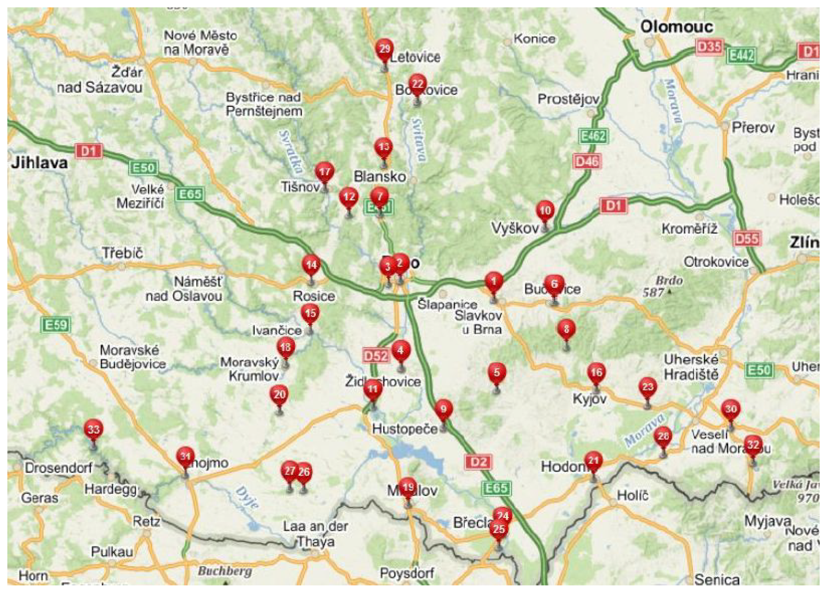
Another example we address involves the reduction in employment offices in the South Moravian Region of the Czech Republic. Due to a significant drop in unemployment, it is necessary to ensure that all villages are within 20 km of the nearest employment office, while maintaining offices in larger towns. The original distribution and the result after the calculated reduction are shown in Figure 1 and Figure 2.

A notable limitation of this work is the absence of capacity considerations for both service centers and customer locations. In practical applications, such as healthcare, logistics, and administrative services, service centers often have limited capacity, and customer demands need to be distributed evenly to prevent overburdening certain centers while underutilizing others. This gap highlights the need to develop a new mathematical model that incorporates capacity management as presented in [13]. However, this updated model primarily focuses on assigning a single customer location to a single service center and does not address the balanced fragmentation of capacities. Balancing constraints ensure that workloads are fairly distributed across centers, while capacity fragmentation allows for splitting customer demands among multiple centers when necessary. These extensions address practical concerns observed in field applications, ensuring both efficiency and service quality. To meet the requirements of scenarios dealing with balanced fragmented capacities, we develop the new model presented in this paper.

Related Work

For more than half a century, covering problems have been a topic of extensive research demonstrating their versatility and importance across a wide range of applications [14,15,16,17,18,19,20,21,22]. These problems have gained significant attention due to their foundational role in addressing real-world challenges, particularly in fields such as logistics and infrastructure planning. According to an analysis of the Scopus database, as of 6 January 2025, a total of 7359 scholarly works on the set covering problem have been published in computer science, mathematics, and engineering, although the lack of support for multi-word queries such as “set covering problem” in Scopus means that the results may include false positives.

The significance of covering problems lies in their ability to support critical decision-making in various domains. For example, they are instrumental in determining optimal locations for essential facilities such as gas stations, schools, factories, landfills, police stations, and even sensor networks. These decisions often impact the efficiency and effectiveness of supply chain operations, showcasing the practical utility of such models. Over the years, researchers have proposed various types of covering problems to address different scenarios. Prominent examples include edge covering [23], vertex covering [24], and capacitated vertex covering [25], among others. Each of these models offers unique methods and perspectives to tackle specific challenges within the overarching framework of covering problems.

This paper narrows its focus to problems that aim to optimize the placement of facilities within designated areas. By examining this subset, the research seeks to contribute to a deeper understanding of how these models can be applied to improve planning and location management, considering balanced fragmented capacity assignments.

For the objectives outlined in the present paper concerning the optimization of static network infrastructure, the foundational model considered is the Location Set Covering Problem (LSCP) along with its various extensions. These extensions are derived from the original set covering problem (SCP) model and consequently inherit similar characteristics, including a focus on achieving minimal computational complexity. Such a property makes these models particularly appealing for large-scale applications where computational efficiency is critical.

Three notable extensions of the capacity-based LSCP framework deal with this context: (i) the CLSCP-CA model, (ii) the CLSCP-EA model, and (iii) the CLSCP-SO model. The CLSCP-CA model pertains to scenarios where the closest service center is designated to handle all requirements at a given customer location, ensuring that demands are met by the most proximate facility. In contrast, the CLSCP-EA model focuses on an equitable distribution of capacities among accessible service centers, aiming to balance the load across the network and prevent the overburdening of any single facility. Lastly, the CLSCP-SO model addresses the assignment of fragmented capacities to customer locations, allowing demands to be fulfilled by distributing resources across multiple facilities when necessary.

An overview of the core mathematical models related to covering problems is provided in

Table 1. An overview of the core mathematical models for covering problems.

Authors	Model	Description	Published
Berge [35]	SCP	The base covering model for all other models. Finding the minimal number of services to cover all demands.	1957
Toregas [14]	LSCP	Extension of SCP considering service and demand locations.	1970
Church et al. [36]	MCLP	Describes the situation of a restricted number of services with the best coverage sought.	1974
Plane and Hendrick [37]	ESS-LSCP	Extension of LSCP addressing the need to consider existing services.	1977
Schilling [38]	LSCP-FT	Extension of LSCP addressing the need for specific demand to be covered by specific services.	1979
Margules [39]	SQ-MCLP	Takes into account the quality of the service provided for each demand.	1986
Current and Storbeck [26]	CLSCP	The first article proposing capacities in LSCP. This model assumes that the demand is split among facilities.	1988
Revelle and Hogan [40]	MALP	Maximizes the availability provided by $\alpha$-reliable coverage.	1989
Gerrard and Church [41]	CLSCP-CA	Models considering services and capacities to satisfy demands using the closest service.	1996
Berman and Krass [42]	GMCLP	Generalized variant of MCLP distinguishing the value of benefits received over a series of coverage ranges.	2002
Dembski and Marks [43]	CLSCP-EA	Models considering services and capacities to equally satisfy demands.	2009
Hong and Kuby [44]	LSCP and MCLP with Threshold	Considers a threshold meaning that each service needs some portion of demand to be viable.	2016
Seda et al. [13]	CLSCP-DA	Consider services and capacities to satisfy demands so that each capacity is assigned to directly and exactly one service.	2020
Hamacher et al. [45]	Extension of LSCP	Addresses the challenge of balancing facility workloads by optimizing co-location strategies within covering problems to improve service efficiency.	2022
Xu et al. [46]	Extension of MCLP	Investigates equity considerations in service allocation within location coverage problems, introducing new metrics and modeling approaches to address disparities.	2023

, which summarizes the key developments in this field. For more detailed explanations of these models, readers are referred to [12,26,27,28,29,30,31,32,33,34].

While previous models have successfully integrated capacities into location-based SCP formulations, they are not fully suited to the specific needs of our problem. To the best of our knowledge, the primary limitations of these existing models arise from assumptions that do not align with the unique constraints posed by modern dynamic systems. Traditional approaches often assume static or one-to-one coverage between demand and service centers, which overlooks the complexities of fragmented demand and the need for strict facility selection in real-world scenarios.

In the light of these gaps, the present paper introduces a new model that better addresses situations where the service capacity must be distributed across overlapping demand regions while respecting realistic operational constraints. Unlike traditional models, which often rely on static or straightforward demand coverage, our model focuses on the challenges related to the fragmented demand allocation and dynamic capacity management in overlapping service areas.

The existing capacity-based LSCP frameworks, such as the CLSCP-CA, CLSCP-EA, and CLSCP-SO models, provide valuable foundations for specific challenges, but they do not fully meet the requirements of the present use case. For example, the CLSCP-CA model’s proximity-based approach assigns all demands from a given location to the closest service center, which can cause overloading when multiple centers need to be used. The CLSCP-EA model, while aiming to balance the load distribution, distributes demand equally among the service centers, which does not necessarily optimize capacity utilization. The CLSCP-SO model, and similar models, to the best of our knowledge, allow for demand to be distributed across centers, but they fail to restrict demand allocation to unselected service centers, which is essential in practical applications. In contrast, the proposed model explicitly ensures that only selected service centers handle the customer demands, preventing unselected centers from being used, and thus, better reflecting real-world constraints.

Another key difference lies in how the demand at each customer location is addressed. While the CLSCP-SO model focuses on satisfying the overall demand through service centers, without enforcing specific allocation for each location, our model ensures that the exact demand from each customer location is fully met by the selected service centers. Additionally, while both models take capacity into account, our model places more emphasis on managing how demand is allocated across overlapping service areas, preventing the overburdening of any single facility. This makes the proposed model particularly well suited for applications that require precise demand fragmentation and capacity balancing.

3. Newly Developed Mathematical Model for Area Coverage Capacity Problems

The original mathematical model for the set covering problem is not directly applicable to the scenarios we are addressing. In our use cases, the optimization of area coverage must account for capacity constraints, which is a crucial aspect in many real-world problems. Specifically, we face the challenge of an unlimited number of customer locations being not able to be assigned to a single service center. For example, in situations where the number of users or devices is constantly increasing—such as in rapidly growing urban areas or in applications such as the Internet of Things (IoT)—this constraint becomes essential. Ignoring this would result in impractical solutions that would not be feasible in real-world settings.

To address this issue, we propose two mathematical models that reflect the following scenarios:

• Each customer location is assigned to exactly one service center.
• Some customer locations may be assigned to multiple service centers simultaneously.

The first model is the basis for our innovative enhancement towards balanced fragmented capacities.

Let us define the following variables, which are used in both mathematical models:

• $c_j,j\in J$: the capacity of service center j;
• $b_i,i\in I$: the number of customers at location i;
• $y_{ij}\in 0,1$: indicates whether customer location i is assigned (1) or not assigned (0) to service center j.

3.1. Each Customer Location Is Assigned Directly to One Service Center

Assume that each customer location is assigned directly to a single service center in the available distance. It is provided by (4).

For a better idea, Figure 3 shows this scenario; here, $S_j$ represents the service center and the circle around his coverage. $L_i$ represents the customer location, where the color indicates to which service center that customer location is assigned.

Based on the above assumptions, we now formulate the model equations:

$$\forall i\in I:\sum _{j\in J}{a}_{ij}{y}_{ij}=1$$

(4)

By (5), each selected service center must have its capacity be sufficient for all the devices from the customer locations that are within the available distance and are assigned to that service center. If a service center is not selected, no customer location can be assigned to it, which is controlled by (6):

$$\forall j\in J:c_j{x}_j\ge \sum _{i\in I}{a}_{ij}{y}_{ij}{b}_i$$

(5)

$$(\forall i\in I)(\forall j\in J):y_{ij}\le x_j$$

(6)

The number of equations in (6) could be reduced. Since

$$\begin{gathered} \forall j\in J:y_{1j}\le x_j \\ \forall j\in J:y_{2j}\le x_j \\ \dots \\ \forall j\in J:y_{mj}\le x_j \end{gathered}$$

summarizing the previous equations, we obtain (7):

$$\forall j\in J:\sum _{i\in I}{y}_{ij}\le m{x}_j$$

(7)

All selected service centers must have a sufficient sum of their capacities to cover all devices (or facilities) from all customer locations. It is expressed by the following Equation (8):

$$\sum _{j\in J}{c}_j{x}_j\ge \sum _{i\in I}{b}_i$$

(8)

However, Equation (8) can be omitted because it follows from Equation (5).

Now, we can summarize all the previous considerations in the following model.

Minimize

$$z=\sum _{j\in J}{w}_j{x}_j$$

(9)

subject to

$$\forall i\in I:\sum _{j\in J}{a}_{ij}{x}_j\ge 1$$

(10)

$$\forall i\in I:\sum _{j\in J}{a}_{ij}{y}_{ij}=1$$

(11)

$$\forall j\in J:c_j{x}_j\ge \sum _{i\in I}{a}_{ij}{y}_{ij}{b}_i$$

(12)

$$\forall j\in J:\sum _{i\in I}{y}_{ij}\le m{x}_j$$

(13)

$$\forall j\in J:x_j\in \{0,1\}$$

(14)

$$(\forall i\in I)(\forall j\in J):y_{ij}\in \{0,1\}$$

(15)

The real-world use case of this model is particularly prevalent in telecommunication networks where the cells of base transceiver stations (BTS) are strictly limited and all devices in the cell are connected directly to a particular BTS. However, interference must be taken into account in this application.

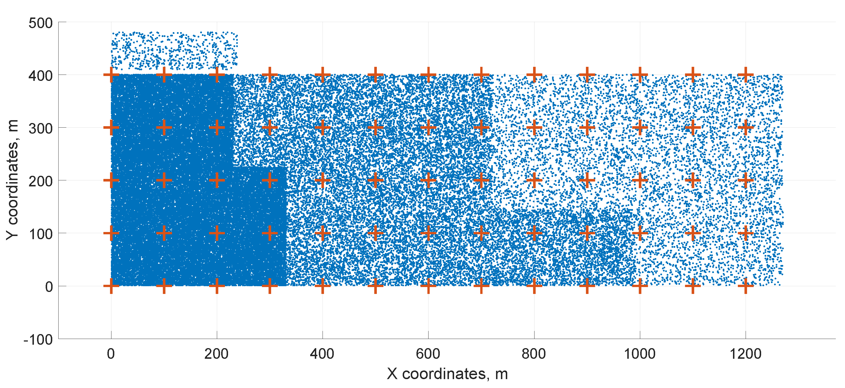
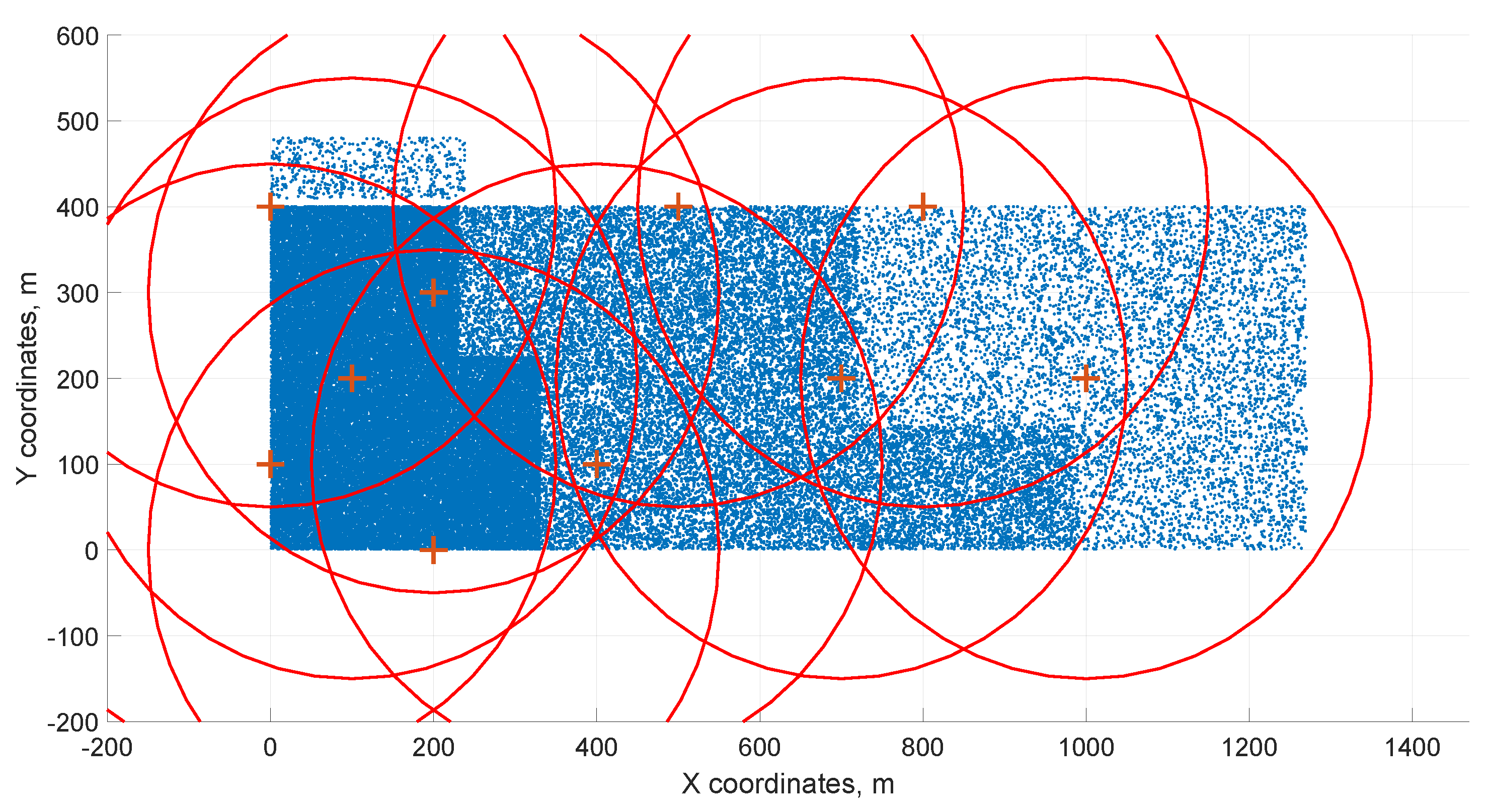
In the specific case of 65 service centers and thousands of customer locations, we examined this situation in the previous article [47], where the model did not take into account the simplification by (13), the meaning of the indices was swapped, and, on the contrary, constraints were added to avoid interference. The initialization distribution of the service centers and the final solution after reduction are shown in Figure 4 and Figure 5. Here, red plus symbols represent service centers, blue points represent customer locations, and red circles represent the service center coverage radii. The optimization reduces the number of service centers from 65 to 10.

Another real-world use case could aim at a different area if we wished to optimize the number of office centers, e.g., financial offices, labor offices, and schools. Here, customer locations (consider city districts or roads) are assigned to a particular office center. For other use cases of the customer location capacities having to be fragmented in the balanced way across selected service centers, we develop a new model presented in Section 3.2.

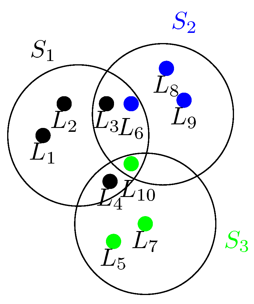
3.2. Each Customer Location Is Assigned to One or More Service Centers

In many real-world applications (e.g., emergency services, healthcare facilities, retail and distribution networks, public transportation systems, energy distribution, education systems, and security systems) one customer location is assigned to more than one service center. For that use case, we create the following mathematical model.

Assume that customers (e.g., persons or devices) from a given location are divided into groups, which are assigned to different centers. The number of customers from location i that will use service center j is denoted by $p_{ij}$. It is clear that $p_{ij}$ have to be non-negative integers and upper bounded by the total number of customers $b_i$ at location i. Therefore, (15) changes to (16):

$$(\forall i\in I)(\forall j\in J):p_{ij}\in {\mathbb{Z}}_{+}$$

(16)

Equation (11) from the previous model is removed, (12) is replaced by (17).

$$\forall j\in J:c_j{x}_j\ge \sum _{i\in I}{a}_{ij}{p}_{ij}$$

(17)

However, it is necessary to satisfy the required numbers of persons from customer locations. This is expressed by (18)

$$\forall i\in I:b_i=\sum _{j\in J}{a}_{ij}{p}_{ij}$$

(18)

The last thing we have to do in the model is to ensure that people cannot be covered from unselected centers. It is necessary to modify Equation (13). The following system of equations ensures this constraint, and at the same time, the fragment values of $p_{ij}$ are upper bounded by $b_i$:

$$(\forall i\in I)(\forall j\in J):p_{ij}\le b_i{x}_j$$

(19)

The upper bound $b_i$ for $p_{ij}$ also follows from Equations (16) and (18). Hence, we see that the system of inequalities (19) can be replaced by the following inequality (20):

$$\forall j\in J:\sum _{i\in I}{p}_{ij}\le \left(\sum _{i\in I}{b}_i\right)x_j$$

(20)

As in the previous model, we do not need Equation (8), as it follows from Equations (17) and (18).

Now, we can summarize the entire modified model with the fragmented coverage of persons from customer locations.

Minimize

$$z=\sum _{j\in I}{w}_j{x}_j$$

(21)

subject to

$$\forall i\in I:\sum _{j\in J}{a}_{ij}{x}_j\ge 1$$

(22)

$$\forall j\in J:c_j{x}_j\ge \sum _{i\in I}{a}_{ij}{p}_{ij}$$

(23)

$$\forall i\in I:b_i=\sum _{j\in J}{a}_{ij}{p}_{ij}$$

(24)

$$\forall j\in J:\sum _{i\in I}{p}_{ij}\le \left(\sum _{i\in I}{b}_i\right)x_j$$

(25)

$$\forall j\in J:x_j\in \{0,1\}$$

(26)

$$(\forall i\in I)(\forall j\in J):p_{ij}\in {\mathbb{Z}}_{+}$$

(27)

The problem is visualized in Figure 6. The customer locations $L_3,L_4,L_6$, and $L_{10}$ are covered by more than one service; thus, it has to be distributed to service centers.

The question now is how to distribute capacities between service centers effectively for the capacities of service centers not be overreached. The implementation perspective and its possible solution are described in Section 4.

3.3. Each Customer Location Is Assigned to One or More Service Centers with Limited Number of Fragments

Above, we discussed the possibility of covering the requirement of customer locations from multiple centers. Such a situation is sometimes directly forced, for example, when the demand of a certain customer location is higher than all the capacities of the centers and, therefore, it is necessary to cover it from multiple centers. This leads to fragmentation.

To adjust the model so that it defines the number of fragments in the capacitated set covering problem, we introduce a new variable to count the fragments, or partial coverage, of customers from different service centers.

The updated model now contains the variables $f_{ij}$ that we will use to calculate the number of fragments to cover the customer locations, $f_{ij}=1$ if $p_{ij}>0$, and 0 otherwise.

Most of the equations remain the same as in model (21)–(27), with just the following constraints (28) and (29) added:

$$(\forall i\in I)(\forall j\in J):f_{ij}=\left\{\begin{array}{cc}1,\hfill & \mathrm{if}{p}_{ij}>0\hfill \\ 0,\hfill & \mathrm{otherwise}\hfill \end{array}\right.$$

(28)

$$(\forall i\in I)(\forall j\in J):f_{ij}\in \{0,1\}$$

(29)

However, Equation (29) can be omitted because the binary values of $f_{ij}$ follow from Equation (28).

We can use the fragment information in two ways.

The first is to modify the objective function by including minimization of the total number of fragments, that is, to minimize

$$z=\sum _{j\in J}{w}_j{x}_j+\sum _{i\in I}\sum _{j\in J}{f}_{ij}$$

(30)

However, when minimizing the total number of fragments, it may happen that some customer locations are covered from a single center and others from a large number of centers.

This can be avoided by limiting the number of fragments to a certain threshold, denoted by $F_{max}$, by omitting the double sum in the objective function, and by adding the following constraint:

$$\forall i\in I:\sum _{j\in J}{f}_{ij}\le F_{max}$$

(31)

4. Complexity and Implementation

The time complexity of the proposed models is essential for the choice of implementation. It will determine whether it is possible to use software for solving tasks with a mixed integer programming model and the assumed maximum size of data structures, or whether it is necessary to use a heuristic method.

4.1. Time Complexity of the First Model

Theorem 1.

The model (9)–(15) runs in $\mathcal{O}\left(2^n\right)$ time.

Proof. 

Since the combination numbers

$$\left({\displaystyle \genfrac{}{}{0pt}{}{n}{k}}\right),k=0,1,\dots ,n$$

indicate how many ways k 1’s can be placed in a binary vector of n elements, by the binomial theorem, the number of all assignments of ones to $x_j\in \{0,1\},j=0,1,\dots ,n$ in Equation (14) is given by

$$\sum _{k=0}^n\left({\displaystyle \genfrac{}{}{0pt}{}{n}{k}}\right)={(1+1)}^n=2^n$$

(32)

For each assignment of $x_j$, the model must verify all constraints:

• Equation (10) requires evaluating ${\sum }_{j\in J}{a}_{ij}{x}_j\ge 1$ for all $i\in I$, which involves $\left|I\right|$ enumeration operations.
• Equations (11)–(13) similarly involve iterating over I and J.
• The worst-case cost of verifying all constraints for one assignment of $x_j$ is proportional to $\left|I\right|\left|J\right|$, where $\left|I\right|=m$ and $\left|J\right|=n$.

Combining the above, the total number of operations is

$$\mathrm{Total}\mathrm{Operations}=2^n\left(\right|I\left|\right|J\left|\right)=2^n\left(mn\right)$$

(33)

Since $mn$ is a polynomial term, which does not affect the exponential growth, the overall time complexity of the model is dominated by $2^n$. Therefore, the time complexity is

$$\mathcal{O}\left(2^n\right)$$

(34)

   □

4.2. Time Complexity of the Second Model

Theorem 2.

The model (21)–(27) runs in $\mathcal{O}\left(2^n\right)$ time.

Proof. 

Similarly to Theorem 1, the number of all assignments of ones to $x_j\in \{0,1\},j=0,1,\dots ,n$ in Equation (26) is given by $2^n$.

For each assignment of $x_j$, the model must verify all constraints:

• Equation (23) requires evaluating $c_j{x}_j\ge {\sum }_{i\in I}{a}_{ij}{p}_{ij}$ for all $j\in J$, which involves $\left|J\right|\left|I\right|$ operations.
• Equation (24) requires evaluating $b_i={\sum }_{j\in J}{a}_{ij}{p}_{ij}$ for all $i\in I$, which involves $\left|I\right|\left|J\right|$ operations.
• Equation (25) requires $\left|I\right|\left|J\right|$ operations.
• Additionally, for each $p_{ij}$, we have to add the constraint $p_{ij}\in {\mathbb{Z}}_{+}$, which imposes integer constraints but does not affect the asymptotic complexity since it is verified in constant time.

The worst-case cost of verifying all constraints for one assignment of $x_j$ is proportional to $\left|I\right|\left|J\right|$, where $\left|I\right|=m$ and $\left|J\right|=n$.

Thus, the total number of operations for all assignments is

$$\mathrm{Total}\mathrm{Operations}=2^n\left(\right|I\left|\right|J\left|\right)=2^n\left(mn\right)$$

(35)

Since $mn$ is a polynomial term and does not affect the exponential growth, the overall time complexity of the model is dominated by $2^n$. Therefore, the time complexity is

$$\mathcal{O}\left(2^n\right)$$

(36)

   □

Obviously, the modification of the second model, indicated in Section 3.3, again has time complexity $\mathcal{O}\left(2^n\right)$.

The set covering problem is NP-hard and, for larger instances, it cannot be exactly solved in an enumerative way and reasonable time as can be seen in

Table 2. Estimated computation time for evaluating $2^n$ operations on an Intel Core i9-13900K processor. This processor has a base frequency of 3.0 GHz and can boost up to 5.8 GHz, assuming an average performance of 10 billion operations per second (10 GFLOPS) to account for overhead and non-ideal conditions.

n	$2^{\mathit{n}}$	Estimated Computation Time
10	$1.024\times {10}^3$	≈ 0.1 μs
20	$1.048\times {10}^6$	≈ 0.1 ms
30	$1.074\times {10}^9$	≈ 0.1 s
40	$1.100\times {10}^{12}$	≈ 110 s
50	$1.126\times {10}^{15}$	≈ 11.6 days
60	$1.153\times {10}^{18}$	≈ 36.5 years
70	$1.181\times {10}^{21}$	≈ 3.75 million years
80	$1.209\times {10}^{24}$	≈ 1208.9 million years
90	$1.238\times {10}^{27}$	$\approx 39.3\mathrm{billion}\mathrm{years}$
100	$1.268\times {10}^{30}$	$\approx 1.27\mathrm{trillion}\mathrm{years}$
200	$1.61\times {10}^{60}$	$\approx 5.1\times {10}^{42}\mathrm{years}$
500	$3.27\times {10}^{150}$	$\approx 1.04\times {10}^{133}\mathrm{years}$
1000	$1.07\times {10}^{301}$	$\approx 3.4\times {10}^{284}\mathrm{years}$

where, for simplicity, we assume that one selection of centers can be generated during one machine instruction. For $n\ge 90$, the computation times exceed the estimated age of the universe, which is approximately 13.8 billion years. This estimation is based on data from the Planck spacecraft, which determined the universe’s age to be about 13.8 billion years [48]. This comparison underscores the impracticality of brute-force solutions for problems with exponential time complexity as n increases. For $n=500$ and $n=1000$, the projected computation times reach astronomical scales far beyond any feasible computational effort. This exponential growth in computational requirements highlights the necessity for more efficient algorithms or heuristic approaches when dealing with such complex problems. Theoretical computer science explores these challenges, particularly through the study of computational complexity and intractability [49].

For this reason, numerous heuristics have been developed [8,10,50,51,52,53,54].

Although the complexity of all models is exponential, our previous implementations for the Steiner tree problem in graphs, graph coloring, maximum clique problem, and the traveling salesman problem show that even for large instances, these problems can be solved in a reasonable amount of time using the GAMS software tool, version 30.2.0 [55]. This tool has built-in deterministic heuristics [55].

To the best of our knowledge, no widely recognized benchmarks exist for capacitated covering problems involving a distance matrix. Therefore, we present computational times in GAMS for the basic set covering problem described by Equations (1)–(3), for which benchmarks are available in the OR-Library [56], with results reported in [50,57]. This is not at the expense of generality, as all the models presented here share the same asymptotic complexity.

Table 3. GAMS computational results.

Benchmark	m	n	Optimal or Best Known Value	Time [s]	Computed Value
scpe1	50	500	5	0.55	5
scpe2	50	500	5	1.09	5
scpe3	50	500	5	1.53	5
scpe4	50	500	5	1.39	5
scpe5	50	500	5	1.52	5
scp41	200	1000	429	0.13	429
scpclr10	511	210	25	3.41	25
scpclr11	1023	330	23	2.83	23
scpclr12	2047	495	26	26.42	23
scpclr13	4095	715	26	208.63	24

summarizes the GAMS results and computation times for 10 benchmark instances selected from these sources.

The first six benchmarks are taken from [50], while the last four are sourced from [57]. The relatively low costs observed in the first five benchmarks result from the highly variable weights (costs) assigned to the centers, which significantly influence the optimal solution. However, [50] does not specify the number or identity of the centers in the optimal solutions.

For instance, in the scp41 benchmark, a minimum total cost of 429 is achieved using 66 centers. If the weights (costs) are disregarded (i.e., all set to 1), 39 centers are selected, with a total cost of 1831. This solution is obtained in 577 s; however, it is already found after 5.92 s and remains unchanged for the remainder of the computation.

In the last four benchmarks, all weights are equal to 1, and thus the result is determined by the number of selected centers. Due to the large values of n, the optimal solutions are unknown; only the best-known solutions are reported.

In the final two cases, GAMS identifies better solutions than those previously reported in [57]. Therefore, we also provide the specific indices of the selected centers for these improved solutions:

• scpclr12: 1, 22, 31, 45, 47, 113, 131, 145, 167, 233, 251, 265, 323, 324, 328, 357, 363, 364, 379, 383, 384, 414, 419.
• scpclr13: 25, 30, 37, 45, 70, 75, 82, 90, 235, 240, 247, 255, 506, 580, 597, 607, 611, 619, 638, 648, 659, 678, 695, 701.

In all cases, the best solution is found quickly, only the last benchmark with complexity $2^{715}$ requiring a little more than 3 min. This, therefore, documents that GAMS is a very good tool for the problems under investigation.

The source code for model (21)–(27) follows. For the first model and the modified second model in this code, only simple modifications are needed, particularly in the declaration sections, the EQUATIONS section, and the DISPLAY statement.

In the calculations, it is first necessary to convert the benchmark data into the GAMS format and for large instances, it is advisable to load them in a form converted from external files using the $INCLUDE externalfilename statement with the full path, e.g.,

$INCLUDE C:\Txt\ARTICLES\2025_Maths\benchmarks\data_SCP1.txt

5. Simulations

In this section, we present the results of the simulations by the previously derived models (9)–(15) and (21)–(27), reflecting real-world constraints and their efficient expression. We first use simple motivation examples to solve the coverage of each demand (i) from a single center, (ii) from multiple centers when the previous approach has no solution, and finally we identify situations of uneven fragmentation, for which we then propose the adapted mathematical model of optimized capacitated coverage with balanced fragmentation. This model is then used on larger instances, and the degree of fragmentation, e.g., the number of fragments generated, is analyzed and the improvements and advantages of our approach in terms of balancing capacity utilization and coverage are highlighted.

5.1. Simulations Based on Created Test Datasets

Let us assume the following distance matrix in

Table 4. Distance matrix.

	1	2	3	4	5
1	28	91	24	36	11
2	47	22	58	47	98
3	124	21	5	168	46
4	8	36	41	34	103
5	17	26	139	46	144
6	74	28	76	36	24
7	23	32	44	82	21
8	128	24	78	5	7

. In all the tables below, the rows represent customer locations, while columns represent service centers.

If $D_{max}=35$, then we obtain the following reachability matrix in

Table 5. Reachability matrix $\left(a_{ij}\right)$.

	1	2	3	4	5
1	1	0	1	0	1
2	0	1	0	0	0
3	0	1	1	0	0
4	1	0	0	1	0
5	1	1	0	0	0
6	0	1	0	0	1
7	1	1	0	0	0
8	0	1	0	1	1

.

For $\mathbf{B}=(18,24,28,29,17,5,13,87)$, $\mathbf{C}=(53,58,22,151,101)$, where all weights are equal to one, the model (9)–(15), where each customer location is assigned to exactly one service center, gives results for $y_{ij}$ as follows in

Table 6. Matrix $\left(y_{ij}\right)$ for model (9)–(15).

	1	2	3	4	5
1	1	0	0	0	0
2	0	1	0	0	0
3	0	1	0	0	0
4	0	0	0	1	0
5	1	0	0	0	0
6	0	1	0	0	0
7	1	0	0	0	0
8	0	0	0	1	0

:

We can see that service centers 1, 2, and 4 are selected (the corresponding columns have a blue background).

In terms of capacities, these assignments correspond to the results as follows in

Table 7. Distribution of sources from service centers to customer locations.

	1	2	3	4	5
1	18	0	0	0	0
2	0	24	0	0	0
3	0	28	0	0	0
4	0	0	0	29	0
5	17	0	0	0	0
6	0	5	0	0	0
7	13	0	0	0	0
8	0	0	0	87	0

.

5.2. Balanced Fragmentation

For comparison, let us assume the same input data and the model (21)–(27), where some customer locations may be assigned to more than one service center simultaneously. It gives the following results.

In

Table 8. Fragmented cover for model (21)–(27).

	1	2	3	4	5
1	18	0	0	0	0
2	0	24	0	0	0
3	0	28	0	0	0
4	0	0	0	29	0
5	16	1	0	0	0
6	0	5	0	0	0
7	13	0	0	0	0
8	0	0	0	87	0

, we can see that three centers are selected (1, 2, and 4), but the customers from the fifth location are divided between two centers disproportionately. To reduce this effect, a constraint has to be added. If r is an “improving” coefficient and n is the number of centers, then we can write the constraint in this way:

$$(\forall i\in I)(\forall j\in J):p_{ij}\ge r{b}_i{x}_j{a}_{ij}/n$$

(37)

The objective function and the constraints of the model (21)–(27) are taken over into the new model without change.

The following tables (see

Table 9. Result for $r=0.1$.

	1	2	3	4	5
1	17				1
2		24
3		28
4	1			28
5	16	1
6		1			4
7	10	2			1
8		2		83	2

,

Table 10. Result for $r=0.5$.

	1	2	3	4	5
1	16		2
2		24
3		8	20
4	3			26
5	7	10
6		5
7	11	2
8		9		78

and

Table 11. Result for $r=0.8$.

	1	2	3	4	5
1	15		3
2		24
3		9	19
4	5			24
5	14	3
6		5
7	10	3
8		14		73

) show the results for $r=0.1$, $r=0.5$, and $r=0.8$, and, for simplicity, only non-zero assignments are included here.

With growing r, the distribution among centers is improved; however, it can be increased only to a specific extent because for each customer, the fragment with the minimum size cannot be larger than his requirement. Therefore, for “too high” r, the problem will have no solution. With regard to constraints (37), the final number of the necessary centers is increased to four. It is evident that, for $r=0$, we obtain the previous model (21)–(27).

Table 12. Results for model (21)–(27), $n_c$ = number of selected centers.

m	n	${\mathit{n}}_{\mathit{c}}$	Maximal Number of Fragments	Fragmented Covers
20	10	5	2	36 + 30, 27 + 37
40	15	7	3	10 + 19, 1 + 12, 17 + 47 + 2, 18 + 46, 5 + 56, 32 + 28, 6 + 9, 4 + 44
60	20	7	2	100 + 4, 100 + 2, 7 + 100, 100 + 5, 92 + 13, 43 + 48, 9 + 100, 100 + 3, 60 + 46, 100 + 6
100	30	8	2	55 + 29, 1 1+ 38, 11 + 52, 100 + 9, 100 + 4, 10 + 64, 4 + 100

summarizes the results by model (21)–(27) for larger instances of the data generated randomly. It can be seen that the number of fragments is low, except for a single case, and it is not greater than two.

In

Table 13. Results for model (21)–(27) and $m=60$, $n=20$.

		${\mathit{c}}_{\mathit{j}}$	560	667	383	874	452	718	792	881	971	573	611	308	632	652	374	720	241	151	846	424
sum	${\mathbf{b}}_{\mathbf{i}}$		1	2	3	4	5	6	7	8	9	10	11	12	13	14	15	16	17	18	19	20
34	34	1													34
12	12	2								12
27	27	3	27
78	78	4						78
77	77	5								77
104	104	6						100							4
102	102	7						100				2
16	16	8													16
91	91	9													91
71	71	10								71
46	46	11										46
95	95	12										95
51	51	13					51
40	40	14										40
35	35	15					35
61	61	16										61
19	19	17								19
107	107	18						7							100
33	33	19													33
105	105	20								100	5
105	105	21					92	13
91	91	22	43				48
98	98	23	98
36	36	24					36
62	62	25					62
57	57	26					57
109	109	27	9									100
31	31	28							31
68	68	29								68
103	103	30									100		3
12	12	31					12
76	76	32													76
93	93	33										93
41	41	34							41
85	85	35	85
17	17	36													17
13	13	37	13
106	106	38									60				46
27	27	39								27
42	42	40								42
37	37	41								37
59	59	42					59
47	47	43								47
94	94	44										94
68	68	45										68
95	95	46	95
106	106	47						100			6
12	12	48	12
63	63	49										63
65	65	50	65
58	58	51						58
25	25	52													25
97	97	53	97
33	33	54						33
75	75	55													75
69	69	56						69
88	88	57						88
16	16	58								16
10	10	59	10
65	65	60								65
		$c_j$	560	667	383	874	452	718	792	881	971	573	611	308	632	652	374	720	241	151	846	424
		sum	554				452	718		876	71	470			517

, for test problem $60\times 20$, for the customer requirements and center capacities given, these results can be seen in more detail. For comparison, the same problem is solved with threshold $r=3.9$ and the results are shown in

Table 14. Results for modified model (21)–(27), (37) and $m=60$, $n=20$, $r=3.9$.

		${\mathit{c}}_{\mathit{j}}$	560	667	383	874	452	718	792	881	971	573	611	308	632	652	374	720	241	151	846	424
sum	${\mathbf{b}}_{\mathbf{i}}$		1	2	3	4	5	6	7	8	9	10	11	12	13	14	15	16	17	18	19	20
34	34	1							7						27
12	12	2	9							3
27	27	3	27
78	78	4						16	62
77	77	5	16				45			16
104	104	6			21			41		21					21
102	102	7			20		42	40
16	16	8													16
91	91	9			18				18						55
71	71	10	14						14	29					14
46	46	11							46
95	95	12	19						38	19					19
51	51	13	10		10		11	10	10
40	40	14	8					32
35	35	15					7		21						7
61	61	16					61
19	19	17						11	4	4
107	107	18						21	21						65
33	33	19		19	7										7
105	105	20							84	21
105	105	21					84	21
91	91	22	18	55			18
98	98	23	20		20			38							20
36	36	24					8		28
62	62	25			13		49
57	57	26			12		12		21						12
109	109	27	47		22					40
31	31	28			7		7	10							7
68	68	29	14							40					14
103	103	30		61			21			21
12	12	31					3	6	3
76	76	32		46			15								15
93	93	33		93
41	41	34						33	8
85	85	35	17				17								51
17	17	36								13					4
13	13	37	10		3
106	106	38			56										50
27	27	39		15	6					6
42	42	40		33						9
37	37	41								37
59	59	42		23	12		12		12
47	47	43	10							37
94	94	44	19		19				56
68	68	45	14	26				14							14
95	95	46	19	19				19	19						19
106	106	47			85			21
12	12	48	3		3		3								3
63	63	49	63
65	65	50	65
58	58	51	12					34	12
25	25	52					5								20
97	97	53	97
33	33	54	7					26
75	75	55		15			15								45
69	69	56	14		14		14								27
88	88	57			18			70
16	16	58					4		4	4					4
10	10	59	8		2
65	65	60					13			52
		$c_i$	560	667	383	874	452	718	792	881	971	573	611	308	632	652	374	720	241	151	846	424
		sum	560	390	383		452	477	488	372					536

. It is clear that the introduction of this threshold reduces the variance of the values of the fragments covering customer needs, but almost all of the coverage of customer needs is composed of fragments. In addition, the number of sources selected is increased by one.

The modification of the second model, outlined in Section 3.3, does not introduce a new quality. The modification of the objective function according to Equation (30) makes the problem a two-criteria one, where the total number of fragments may exceed the number of selected centers and the weights of the subcriteria would still need to be solved.

In simulations with the threshold $F_{max}$, it turns out that this number of fragments is almost always used in the results, which leads to a large fragmentation at larger values of this threshold and, for a low value, we obtain a solution obtained by model (21)–(27), and for $F_{max}=1$, we obtain a solution according to model (9)–(15).

6. Conclusions

In this paper, we present newly developed mathematical models for area coverage capacity problems, designed to address challenges in optimizing service center placements and capacity allocation. These models consider critical factors such as required capacities for specific areas and the need to manage multiple service centers serving the same location, ensuring efficient and balanced coverage. The proposed approach offers flexibility in handling various real-world scenarios where customer demand may be fragmented across multiple service centers while adhering to operational constraints.

The models have been validated through a series of simulations, and the results demonstrate their applicability and effectiveness in optimizing resource allocation. The simulations have confirmed that the models are robust and well suited for practical implementation, providing valuable insights into capacity management and demand distribution in various use cases. Additionally, the data representation provided in the paper ensures that these models can be easily integrated into the existing planning and optimization software, and, as it has been shown, even large instances of covering problems can be solved in GAMS.

However, it is important to acknowledge some limitations of the proposed models. They currently assume static demands, which may not reflect the dynamic nature of customer needs in certain contexts. Future research could address these limitations by incorporating dynamic demand models and exploring decomposition techniques to improve scalability.

Beyond these limitations, the broader societal and economic implications of this research are significant. By improving the efficiency of capacity allocation and ensuring that service centers are optimally placed, the proposed models could contribute to more equitable access to essential services, such as healthcare and education. Specifically, the ability to balance service fragmentation across multiple centers could help reduce operational costs and increase the overall efficiency of critical infrastructure. In public health, for example, optimizing the location and capacity of healthcare facilities could reduce patient waiting times, improve emergency response times, and enhance healthcare accessibility in underserved regions. This research has the potential to contribute to more sustainable and cost-effective public infrastructure planning, ultimately leading to improved societal outcomes.

Looking ahead, future research will focus on extending the models to handle even more complex scenarios. Specifically, we plan to integrate stochastic demand models to account for uncertainties in demand, which would improve the models’ adaptability to real-world situations where customer needs can fluctuate. Another important direction for future work involves exploring additional objectives to allow, for instance, for the balance between minimizing operational costs while maximizing service quality. Additionally, we will investigate the use of decomposition techniques to address scalability issues, allowing the models to efficiently handle larger and more complex instances. By incorporating these advancements, we aim to further improve the practical applicability of the models and extend their utility in diverse service allocation contexts.