Modified Kibria–Lukman Estimator for the Conway–Maxwell–Poisson Regression Model: Simulation and Application

Abstract

This study presents a novel estimator that combines the Kibria–Lukman and ridge estimators to address the challenges of multicollinearity in Conway–Maxwell–Poisson (COMP) regression models. The Conventional COMP Maximum Likelihood Estimator (CMLE) is notably susceptible to the adverse effects of multicollinearity, underscoring the necessity for alternative estimation strategies. We comprehensively compare the proposed COMP Modified Kibria–Lukman estimator (CMKLE) against existing methodologies to mitigate multicollinearity effects. Through rigorous Monte Carlo simulations and real-world applications, our results demonstrate that the CMKLE exhibits superior resilience to multicollinearity while consistently achieving lower mean squared error (MSE) values. Additionally, our findings underscore the critical role of larger sample sizes in enhancing estimator performance, particularly in the presence of high multicollinearity and over-dispersion. Importantly, the CMKLE outperforms traditional estimators, including the CMLE, in predictive accuracy, reinforcing the imperative for judicious selection of estimation techniques in statistical modeling.

1. Introduction

Generalized linear models (GLMs) are powerful tools for modeling relationships between explanatory variables (predictors) and response variables, extending traditional linear regression to accommodate various data types, including those following distributions within the exponential family [1]. A key application of GLMs is modeling count data, which arises in social sciences, healthcare, economics, auto insurance claims, and medical research. Unlike continuous data, count data are discrete and often exhibit patterns of dispersion that complicate standard modeling approaches [2,3]. Several specialized GLMs have been developed, including Poisson and negative binomial regression models, to model count data [4,5].

Each model has strengths and limitations, depending on the specific data characteristics. The Poisson regression model, for instance, is commonly used for discrete data but assumes that the mean and variance are equal (equi-dispersion). This assumption is rarely held in practice, as count data often exhibit greater variability (over-dispersion), necessitating alternatives like the negative binomial model [2]. The negative binomial regression model addresses over-dispersion by introducing a dispersion parameter that allows for a variance greater than the mean, making it more suitable for real-world applications. However, the negative binomial model is limited to over-dispersed data and cannot accommodate under-dispersion, where the variance is less than the mean. In contrast, the COM–Poisson regression model offers greater flexibility by handling over-dispersion and under-dispersion [6,7]. This versatility allows it to be applied across a broader range of count data scenarios. The COM–Poisson distribution, introduced by Conway and Maxwell [7], generalizes the Poisson distribution and includes the geometric, Poisson, and Bernoulli distributions as special cases, making it increasingly popular for count data analysis.

In recent studies, the Conway–Maxwell–Poisson (COM–Poisson or COMP) regression model has gained considerable attention due to its ability to accommodate data with varying levels of dispersion [8,9]. This flexibility makes it a robust alternative to traditional models such as the Poisson and negative binomial regression models, which are limited to handling equi-dispersion and over-dispersion. The COMP model is useful when dealing with count data that exhibit complex dispersion patterns, as it can model over-dispersion (variance greater than the mean) and under-dispersion (variance less than the mean). This versatility has led to its growing adoption and has attracted increasing attention in recent research. The parameters of the COM–Poisson model are typically estimated using the COM–Poisson Maximum Likelihood Estimator (CMLE). However, the CMLE has a notable limitation: it becomes inefficient and produces unstable estimates in multicollinearity, a common issue where the explanatory variables are highly correlated [10,11]. Multicollinearity can inflate the variance of parameter estimates, leading to unreliable inference and predictions.

To address this issue, researchers have developed alternative estimators, which can mitigate the impact of multicollinearity by introducing a bias that stabilizes the estimates. Among these alternatives are the COM–Poisson Ridge estimator (CRE) [11], COM–Poisson Liu estimator (CLE) [12], COM–Poisson Liu-type estimator (CLTE) [9], and the COM–Poisson Kibria–Lukman estimator (CKLE) [8], among others. These shrinkage estimators combine the robustness of the COM–Poisson model with strategies to handle multicollinearity, thereby providing more stable and efficient parameter estimates. Each of these estimators has its strengths depending on the severity of multicollinearity and the specific structure of the data. For instance, the CRE introduces a penalty proportional to the size of the coefficients, effectively shrinking them towards zero to reduce variance. The CLE and CLTE, on the other hand, adjust the bias–variance trade-off more finely, making them particularly useful when the multicollinearity is moderate.

Recent advancements in alternative estimation techniques have helped mitigate the effects of multicollinearity in the COMP regression model, leading to more stable parameter estimates. As research in this field continues to evolve, the COMP model combined with shrinkage estimators shows great potential for applications involving count data, particularly in scenarios where multicollinearity exists among explanatory variables. Aladeitan et al. [13] introduced the Modified Kibria–Lukman (MKL) estimator to address multicollinearity in Poisson regression, showing that the MKL outperforms the Poisson Maximum Likelihood Estimator (PMLE), Poisson Ridge Regression Estimator (PRE), Poisson Liu Estimator (PLE), and Poisson Kibria–Lukman (PKL) estimator.

This paper aims to extend these methodologies by proposing a new COMP Modified Kibria–Lukman Estimator (COMP-MKL) as an alternative for handling multicollinearity in the COMP regression model. We will compare the performance of the proposed COMP-MKL estimator with existing estimators such as the CRE, CLE, CKLE, and CLTE using the scalar mean squared error (SMSE) criterion. Theoretical findings will be substantiated through simulation studies and real data analysis to demonstrate the superior performance of the proposed estimator over its competitors.

The paper is structured as follows: Section 2 outlines the fundamentals of the COMP regression model, reviews existing estimators, and introduces the new COMP-MKL estimator. Section 3 presents a theoretical comparison of the proposed estimator with its competitors. Section 4 reports the results of an extensive Monte Carlo simulation study, assessing the performance of the proposed and competing estimators based on the MSE criteria. Section 5 showcases a real-world data example that further validates the superiority of the proposed estimator. Section 6 provides concluding remarks, summarizing the key findings and implications for future research.

2. COMP Regression Model and Estimation

The Conway–Maxwell–Poisson (COMP) distribution, introduced by Conway and Maxwell [7], is a versatile distribution designed to handle both over-dispersed and under-dispersed count data, addressing the limitations of the traditional Poisson distribution. Its probability mass function (pmf) is given as follows:

$$P\left(Y=y|\lambda ,\nu \right)={\displaystyle \frac{{\lambda }^y}{{(y!)}^{\nu }Z\left(\lambda ,\nu \right)}}, y=\mathrm{0,1},2,\dots$$

(1)

where $\lambda$ is the rate parameter, $\nu$ is the dispersion parameter, and $Z\left(\lambda ,\nu \right)$ is the normalizing constant. The flexibility of the COMP distribution stems from the dispersion parameter, allowing it to model a range of distributions, from Poisson (when $\nu =1$) to Bernoulli-like (as $\nu \to \infty$) to geometric (when $\nu =0$).

The COM–Poisson regression model, introduced by Sellers and Shmueli [14], incorporates this distribution to model count data with varying levels of dispersion. The expected value of the COMP distribution can be approximated as follows:

$$E\left(Y\right)\approx {\lambda }^{{\displaystyle \frac{1}{\nu }}}+{\displaystyle \frac{1}{2\upsilon }}-0.5$$

(2)

while the variance is similarly expressed as follows:

$$V\left(Y\right)\approx {\displaystyle \frac{1}{\upsilon }}{\lambda }^{{\displaystyle \frac{1}{\nu }}}$$

(3)

The COMP regression model is a generalized linear model with a mean link function, typically the log link function:

$$log\left({\mu }_i\right)=x_i^T\beta , i=\mathrm{1,2},\dots ,n$$

(4)

where ${\mu }_i$ is the expected count, $x_i$ is a vector of covariates, and $\beta$ is the corresponding vector of regression coefficients. The dispersion parameter can be either fixed or modeled as a function of covariates. Given the nonlinear nature of the likelihood function in COMP regression, maximum likelihood estimation (MLE) requires iterative optimization methods. The log-likelihood function for the COMP regression model is expressed as follows:

$$\mathcal{l}\left(\beta \right)={\sum }_{i=1}^n\left(y_{i}log\left({\lambda }_i\right)-\upsilon log\left(y_i!\right)\right)-{\sum }_{i=1}^{n}logZ\left({\lambda }_i,\upsilon \right)$$

(5)

where ${\lambda }_i=\mathrm{e}\mathrm{x}\mathrm{p}\left(x_i^T\beta \right)$ is the rate parameter. Since the likelihood is nonlinear in $\beta$, iterative algorithms like iteratively reweighted least squares (IRLSs) or Newton–Raphson methods are employed to find the CMLE of $\beta$. The CMLE ${\widehat{\beta }}_{CMLE}$ is obtained by solving the following:

$${\widehat{\beta }}_{CMLE}={\left(X^T\widehat{W}X\right)}^{-1}{X}^T\widehat{W}\widehat{z}$$

(6)

where the weight matrix $\widehat{W}$ is based on the second derivative of the log-likelihood and $\widehat{z}$ is the adjusted response variable. For a more comprehensive treatment of the derivation and implementation of the CMLE, refer to [8,9]. The MLE is consistent and asymptotically efficient but possesses high variance and instability when multicollinearity is present in the model. Consequently, biased estimation methods such as CRE, CLE, and CKLE are often preferred over the CMLE.

The mean squared error (SMSE) of the CMLE is given as follows:

$${MSE(\widehat{\beta }}_{CMLE})={\widehat{\upsilon }\left(X^T\widehat{W}X\right)}^{-1}$$

(7)

When multicollinearity is present, the weighted cross-product matrix of the design matrix ($X^T\widehat{W}X$) becomes poorly conditioned, leading to instability in the coefficient estimates obtained from the conventional CMLE. To address this issue, shrinkage estimators provide a robust alternative by introducing regularization, stabilizing the regression estimates, and reducing the effects of multicollinearity. The following section will review several existing shrinkage methods specifically developed for the COMP regression model and discuss their theoretical properties and practical applications.

2.1. Shrinkage Estimators

To tackle the issue of multicollinearity in linear regression, several shrinkage estimators have been introduced, including the ridge regression estimator by Hoerl and Kennard [15], as well as the Liu and Liu-type estimators [16,17], the Kibria–Lukman estimator [18], and two-parameter estimators [19,20]. These methods have been adapted to address multicollinearity in generalized linear models, extending their application to models such as Poisson regression [4,21], negative binomial regression (NBR) [5,22], and the Conway–Maxwell–Poisson (COMP) regression model [5,6,23]. These extensions have proven effective in maintaining estimator stability in the presence of highly collinear predictors.

Sami et al. [11] developed the COMP ridge estimator (CRE) and defined it as follows:

$${\widehat{\beta }}_{CRE}=D^{-1}{X}^{\prime }\widehat{W}X{\widehat{\beta }}_{CMLE}, \mathrm{k}>0,$$

(8)

where ${D=X}^{\prime }\widehat{W}X+kI,$ and k is the ridge parameter, defined in this study as $k=\sqrt{{\displaystyle \frac{p}{\mathrm{sum}\left({\widehat{\beta }}_{CMLE}^2\right)}}}$. The matrix mean squared error (MMSE) is expressed as follows:

$$\mathrm{M}\mathrm{M}\mathrm{S}\mathrm{E}\left({\widehat{\beta }}_{CRE}\right)={\widehat{\upsilon }\mathrm{D}}^{-1}{X}^{\prime }\widehat{W}X{D}^{-1}+k^2{\left(D\right)}^{-1}{\beta {\beta }^T\left(D\right)}^{-1}.$$

(9)

Akram et al. [12] expanded the application of the Liu estimator (LE) to the COMP regression model in the following way:

$${\widehat{\beta }}_{CLE}=C_d{\widehat{\beta }}_{CMLE}, 0<\mathrm{d}<1,$$

(10)

where $C_d={\left(X^{\prime }\widehat{W}X+I\right)}^{-1}\left(X^{\prime }\widehat{W}X+\mathrm{d}I\right)$. The Liu parameter d in this study is defined as $d={\displaystyle \frac{1}{\mathrm{m}\mathrm{i}\mathrm{n}\left({\widehat{\beta }}_{CMLE}^2\right)}}$. The MMSE is expressed as follows:

$$\mathrm{M}\mathrm{M}\mathrm{S}\mathrm{E}\left({\widehat{\beta }}_{CLE}\right)=\widehat{\upsilon }{C}_d{{\left(X^{\prime }\widehat{W}X\right)}^{-1}C}_d+{(1-d)}^2{\left(X^{\prime }\widehat{W}X+I\right)}^{-1}\beta {\beta }^T{\left(X^{\prime }\widehat{W}X+I\right)}^{-1}.$$

(11)

Kibria and Lukman [18] introduced a ridge-type estimator as an effective solution to the problem of multicollinearity in linear regression. Recognizing the need for similar strategies in more complex models, Abonazel et al. [8] extended this approach to the COMP regression model, resulting in what is now referred to as the COMP Kibria–Lukman estimator (CKLE). This estimator is designed to address multicollinearity by balancing bias and variance through regularization, thereby improving the stability of estimates in the COMP model. The CKLE is defined as follows:

$${\widehat{\beta }}_{CKLE}=C_k{\widehat{\beta }}_{CMLE}, 0<\mathrm{k}<1,$$

(12)

where $C_k={\left(X^{\prime }\widehat{W}X+kI\right)}^{-1}\left(X^{\prime }\widehat{W}X-\mathrm{k}I\right)$. The MMSE is expressed as follows:

$$\mathrm{M}\mathrm{M}\mathrm{S}\mathrm{E}\left({\widehat{\beta }}_{CKLE}\right)=\widehat{\upsilon }{C}_k{{\left(X^{\prime }\widehat{W}X\right)}^{-1}C}_k+{4k}^2{\left(X^{\prime }\widehat{W}X+kI\right)}^{-1}\beta {\beta }^T{\left(X^{\prime }\widehat{W}X+kI\right)}^{-1}.$$

(13)

Liu [16] introduced the Liu-type estimator to address multicollinearity in linear regression, merging the strengths of both the ridge and Liu estimators. This hybrid approach leverages the benefits of reduced variance and controlled bias. Building on this concept, Tanış and Asar [9] extended the Liu-type estimator to the Conway–Maxwell–Poisson (COMP) regression model, referred to as the COMP Liu-type estimator (CLTE). The formulation of this estimator is as follows:

$${\widehat{\beta }}_{CLTE}=C_{kd}{\widehat{\beta }}_{CMLE}, \mathrm{k}>0,0<\mathrm{d}<1,$$

(14)

where $C_{kd}={\left(X^{\prime }\widehat{W}X+kI\right)}^{-1}\left(X^{\prime }\widehat{W}X-\mathrm{d}I\right)$. The MMSE is expressed as follows:

$$\mathrm{M}\mathrm{M}\mathrm{S}\mathrm{E}\left({\widehat{\beta }}_{CLTE}\right)=\widehat{\upsilon }{C}_{kd}{{\left(X^{\prime }\widehat{W}X\right)}^{-1}C}_{kd}+{(k+d)}^2{\left(X^{\prime }\widehat{W}X+kI\right)}^{-1}\beta {\beta }^T{\left(X^{\prime }\widehat{W}X+kI\right)}^{-1}.$$

(15)

Sami et al. [23] introduced a two-parameter estimator for the Conway–Maxwell–Poisson (COMP) regression model, building upon the work of Asar and Genc [21]. This estimator, known as the two-parameter estimator (CTPE), was designed to provide greater flexibility in handling multicollinearity by incorporating two tuning parameters. The CTPE estimator is defined as follows:

$${\widehat{\beta }}_{CTPE}=H_{kd}{\widehat{\beta }}_{CMLE}, \mathrm{k}>0,0<\mathrm{d}<1,$$

(16)

where $H_{kd}={\left(X^{\prime }\widehat{W}X+kI\right)}^{-1}\left(X^{\prime }\widehat{W}X+\mathrm{k}\mathrm{d}I\right)$. The MMSE is expressed as follows:

$$\mathrm{M}\mathrm{M}\mathrm{S}\mathrm{E}\left({\widehat{\beta }}_{CTPE}\right)=\widehat{\upsilon }{H}_{kd}{{\left(X^{\prime }\widehat{W}X\right)}^{-1}H}_{kd}+k^2{(d-1)}^2{\left(X^{\prime }\widehat{W}X+kI\right)}^{-1}\beta {\beta }^T{\left(X^{\prime }\widehat{W}X+kI\right)}^{-1}$$

(17)

Additionally, Sami et al. [23] developed a two-parameter estimator for the Conway–Maxwell–Poisson (COMP) regression model, drawing from the work of Huang and Yang [22] on negative binomial regression (NBRM). This new estimator, the COMP Huang and Yang estimator (CHYE), was designed to extend the flexibility of biased estimation methods to the COMP framework. The CHYE is defined as follows:

$${\widehat{\beta }}_{CHYE}=M_{kd}{X}^{\prime }\widehat{W}X{\widehat{\beta }}_{CMLE}, \mathrm{k}>0,0<\mathrm{d}<1,$$

(18)

where $M_{kd}={\left(X^{\prime }\widehat{W}X+I\right)}^{-1}\left(X^{\prime }\widehat{W}X+\mathrm{d}I\right){\left(X^{\prime }\widehat{W}X+kI\right)}^{-1}$. The MMSE is expressed as follows:

$$\mathrm{M}\mathrm{M}\mathrm{S}\mathrm{E}\left({\widehat{\beta }}_{CHYE}\right)=\widehat{\upsilon }{M}_{kd}{X^{\prime }\widehat{W}XM}_{kd}+G{N}_{kd}\beta {\beta }^{T}G{N}_{kd},$$

(19)

where $N_{kd}={\left(X^{\prime }\widehat{W}X+I\right)}^{-1}{\left(X^{\prime }\widehat{W}X+kI\right)}^{-1}$ and $G=\left(k-d+1\right)X^{\prime }\widehat{W}X+kI$.

2.2. Proposed Estimator

In this study, we introduce a new estimator that builds upon the work of Aladeitan et al. [13], who proposed the Modified Kibria–Lukman estimator specifically for the Poisson regression model. The estimator inherits the advantage of the Kibria–Lukman estimator with the ridge estimator. While many of the estimators discussed earlier can be classified as either single-parameter or two-parameter methods, the Modified Kibria–Lukman estimator, despite having a single biasing parameter, demonstrates superior performance compared to some two-parameter estimators. Recognizing the potential of this approach, we extended it to the Conway–Maxwell–Poisson (COMP) regression model, developing what we call the COMP Modified Kibria–Lukman estimator (CMKLE). The CMKLE offers improved estimator stability and accuracy in scenarios where traditional estimators may struggle due to high collinearity among predictor variables. The CMKLE is defined as follows:

$${\widehat{\beta }}_{CMKLE}=C_k{\widehat{\beta }}_{CRE}, 0<\mathrm{k}<1.$$

(20)

where $C_k={\left(X^{\prime }\widehat{W}X+kI\right)}^{-1}\left(X^{\prime }\widehat{W}X-\mathrm{k}I\right)$. The bias of the estimator is expressed as follows:

$$\mathrm{B}\mathrm{i}\mathrm{a}\mathrm{s}\left({\widehat{\beta }}_{CKLE}\right)=-k{D}^{-1}F{D}^{-1}\beta$$

(21)

where $F=\left({3X}^{\prime }\widehat{W}X+kI\right).$ The covariance matrix is defined as follows:

$$\mathrm{C}\mathrm{o}\mathrm{v}\left({\widehat{\beta }}_{CMKLE}\right)=\widehat{\upsilon }{C}_k{D^{-1}{X}^{\prime }\widehat{W}X{D}^{-1}C}_k$$

(22)

Hence, the MMSE is expressed as follows:

$$\mathrm{C}\mathrm{o}\mathrm{v}\left({\widehat{\beta }}_{CMKLE}\right)=\widehat{\upsilon }{C}_k{D^{-1}{X}^{\prime }\widehat{W}X{D}^{-1}C}_k+k^2{D}^{-2}F\beta {\beta }^{T}F{D}^{-2}$$

(23)

Let $Q^{\ast T}\left(X^{\prime }\widehat{W}X\right)Q^{\ast }=\mathrm{E}=diag\left\{e_j\right\}$, $\mathrm{j}=\mathrm{1,2},\dots ,p$, where $e_1\ge e_2\ge \dots \ge e_{p^{\mathrm{*}}}$ are the ordered eigenvalues of $X^{\prime }\widehat{W}X$ and $Q^{\ast }$ is $p \times p$ matrix whose columns of the normalized eigenvectors of $X^{\prime }\widehat{W}X$. Thus, we can express $\beta$ in terms of $\theta$, then ${\widehat{\theta }}_{CMLE}=Q^{\ast T}{\widehat{\beta }}_{CMLE}$, leading to the canonical form of the CMLE. Consequently, we expressed other equations in this study in canonical form:

$${\widehat{\theta }}_{CRE}={\left(\mathrm{E}+kI\right)}^{-1}\mathrm{E}{\widehat{\theta }}_{CMLE}.$$

(24)

$${\widehat{\theta }}_{CLE}={\left(\mathrm{E}+I\right)}^{-1}\left(\mathrm{E}+\mathrm{d}I\right){\widehat{\theta }}_{CMLE.}$$

(25)

$${\widehat{\theta }}_{CKLE}={\left(\mathrm{E}+\mathrm{k}I\right)}^{-1}\left(\mathrm{E}-\mathrm{k}I\right){\widehat{\theta }}_{CMLE}.$$

(26)

$${\widehat{\theta }}_{CLTE}={\left(\mathrm{E}+\mathrm{k}I\right)}^{-1}\left(\mathrm{E}-\mathrm{d}I\right){\widehat{\theta }}_{CMLE}.$$

(27)

$${\widehat{\theta }}_{CTPE}={\left(\mathrm{E}+\mathrm{k}I\right)}^{-1}\left(\mathrm{E}+\mathrm{k}\mathrm{d}I\right){\widehat{\theta }}_{CMLE}.$$

(28)

$${\widehat{\theta }}_{CHYE}={\left(\mathrm{E}+I\right)}^{-1}\left(\mathrm{E}+dI\right){\left(\mathrm{E}+\mathrm{k}I\right)}^{-1}\mathrm{E}{\widehat{\theta }}_{CMLE}.$$

(29)

$${\widehat{\theta }}_{CMKLE}={\left(\mathrm{E}+\mathrm{k}I\right)}^{-1}\left(\mathrm{E}-\mathrm{k}I\right){\left(\mathrm{E}+\mathrm{k}I\right)}^{-1}\mathrm{E}{\widehat{\theta }}_{CMLE}.$$

(30)

Furthermore, for ease of computation, we applied the same shrinkage parameters across all estimators in this study. This approach ensured an impartial and uniform comparison without favoring any estimator. Specifically, the ridge parameters k and d are defined as $k=\sqrt{{\displaystyle \frac{p}{\mathrm{sum}\left({\widehat{\beta }}_{CMLE}^2\right)}}}$ and $={\displaystyle \frac{1}{\mathrm{m}\mathrm{i}\mathrm{n}\left({\widehat{\beta }}_{CMLE}^2\right)}},$ respectively.

We can also evaluate the performance of the estimators using the scalar mean squared error (SMSE) instead of the MMSE. The SMSE is defined as follows:

$$\mathrm{S}\mathrm{M}\mathrm{S}\mathrm{E}\left(\vartheta \right)=tr\left[Cov\left(\tilde{\vartheta }\right)\right]+\mathrm{t}\mathrm{r}\left[bias\left(\tilde{\vartheta }\right)bias{\left(\vartheta \right)}^{\prime }\right]$$

(31)

where $Cov\left(\tilde{\vartheta }\right)$ is the covariance matrix of $\tilde{\vartheta }$ and $bias\left(\tilde{\vartheta }\right)=E\left(\tilde{\vartheta }\right)-\tilde{\vartheta }$. This formulation allows us to express the matrix mean squared error in a scalar form by summing the trace of the covariance and the trace of the squared bias, making it easier to compare the performances of different estimators. Consequently, we reformulate the MMSE of all the estimators in terms of the SMSE for a more concise comparison. The SMSEs of the mentioned estimators above are obtained as follows:

$$\mathrm{S}\mathrm{M}\mathrm{S}\mathrm{E}\left({\widehat{\theta }}_{CMLE}\right)=\widehat{\upsilon }{\sum }_{j=1}^p{\displaystyle \frac{1}{e_j}}.$$

(32)

$$\mathrm{S}\mathrm{M}\mathrm{S}\mathrm{E}\left({\widehat{\theta }}_{CRE}\right)=\widehat{\upsilon }{\sum }_{j=1}^p{\displaystyle \frac{e_j}{{\left(e_j+k\right)}^2}}+{\sum }_{j=1}^p{\displaystyle \frac{{\theta }_j^2{k}^2}{{\left(e_j+k\right)}^2}}.$$

(33)

$$\mathrm{S}\mathrm{M}\mathrm{S}\mathrm{E}\left({\widehat{\theta }}_{CLE}\right)=\widehat{\upsilon }{\sum }_{j=1}^p{\displaystyle \frac{{(e_j+d)}^2}{{\left(e_j+1\right)}^2{e}_j}}+{(d-1)}^2{\sum }_{j=1}^p{\displaystyle \frac{{\theta }_j^2}{{\left(e_j+1\right)}^2}}.$$

(34)

$$\mathrm{S}\mathrm{M}\mathrm{S}\mathrm{E}\left({\widehat{\theta }}_{CKLE}\right)=\widehat{\upsilon }{\sum }_{j=1}^p{\displaystyle \frac{{(e_j-k)}^2}{{\left(e_j+k\right)}^2{e}_j}}+4k^2{\sum }_{j=1}^p{\displaystyle \frac{{\theta }_j^2}{{\left(e_j+k\right)}^2}}.$$

(35)

$$\mathrm{S}\mathrm{M}\mathrm{S}\mathrm{E}\left({\widehat{\theta }}_{CLTE}\right)=\widehat{\upsilon }{\sum }_{j=1}^p{\displaystyle \frac{{(e_j-d)}^2}{{\left(e_j+k\right)}^2{e}_j}}+{(d+k)}^2{\sum }_{j=1}^p{\displaystyle \frac{{\theta }_j^2}{{\left(e_j+k\right)}^2}}.$$

(36)

$$\mathrm{S}\mathrm{M}\mathrm{S}\mathrm{E}\left({\widehat{\theta }}_{CTPE}\right)=\widehat{\upsilon }{\sum }_{j=1}^p{\displaystyle \frac{{(e_j+kd)}^2}{{\left(e_j+k\right)}^2{e}_j}}+k^2{(d-1)}^2{\sum }_{j=1}^p{\displaystyle \frac{{\theta }_j^2}{{\left(e_j+k\right)}^2}}.$$

(37)

$$\mathrm{S}\mathrm{M}\mathrm{S}\mathrm{E}\left({\widehat{\theta }}_{CHYE}\right)=\widehat{\upsilon }{\sum }_{j=1}^p{\displaystyle \frac{{e_j(e_j+d)}^2}{{\left(e_j+1\right)}^2{\left(e_j+k\right)}^2}}+{\sum }_{j=1}^p{\displaystyle \frac{{\left({(1+k-d)e}_j+k\right)}^2{\theta }_j^2}{{\left(e_j+k\right)}^2{\left(e_j+1\right)}^2}}.$$

(38)

$$\mathrm{S}\mathrm{M}\mathrm{S}\mathrm{E}\left({\widehat{\theta }}_{CMKLE}\right)=\widehat{\upsilon }{\sum }_{j=1}^p{\displaystyle \frac{{e_j(e_j-k)}^2}{{\left(e_j+k\right)}^4}}+k^2{\sum }_{j=1}^p{\displaystyle \frac{{\left({3e}_j+k\right)}^2{\theta }_j^2}{{\left(e_j+k\right)}^4}}.$$

(39)

3. Theoretical Comparisons

3.1. CMKLE and CMLE

The estimator ${\widehat{\theta }}_{CMKLE}$ is superior to the estimator ${\widehat{\theta }}_{CMLE}$ in the sense of the SMSE criterion, i.e., SMSE$\left({\widehat{\theta }}_{CMKLE}\right)-SMSE\left({\widehat{\theta }}_{CMLE}\right)<0$ for $\widehat{\upsilon }$> 0 and $k>0$ if ${e_j^2(e_j-k)}^2+\widehat{\upsilon }{k}^2{\left({3e}_j+k\right)}^2{\theta }_j^2{e}_j<{\left(e_j+k\right)}^4.$

Proof. 

The difference between $SMSE\left({\widehat{\theta }}_{CMKLE}\right) \mathrm{a}\mathrm{n}\mathrm{d} SMSE\left({\widehat{\theta }}_{CMLE}\right)$ is obtained as follows:

$$\begin{gathered} {∆}_1=SMSE\left({\widehat{\theta }}_{CMKLE}\right)-SMSE\left({\widehat{\theta }}_{CMLE}\right) \\ {∆}_1=\widehat{\upsilon }{\sum }_{j=1}^p{\displaystyle \frac{{e_j(e_j-k)}^2}{{\left(e_j+k\right)}^4}}+k^2{\sum }_{j=1}^p{\displaystyle \frac{{\left({3e}_j+k\right)}^2{\theta }_j^2}{{\left(e_j+k\right)}^4}}-\widehat{\upsilon }{\sum }_{j=1}^p{\displaystyle \frac{1}{e_j}} \\ {∆}_1=\widehat{\upsilon }{\sum }_{j=1}^p{\displaystyle \frac{{e_j^2(e_j-k)}^2+\widehat{\upsilon }{k}^2{\left({3e}_j+k\right)}^2{\theta }_j^2{e}_j-{\left(e_j+k\right)}^4}{e_j{\left(e_j+k\right)}^4}} \end{gathered}$$

(40)

The difference ${∆}_1$ < 0 if ${e_j^2(e_j-k)}^2+\widehat{\upsilon }{k}^2{\left({3e}_j+k\right)}^2{\theta }_j^2{e}_j<{\left(e_j+k\right)}^4$ for $\widehat{\upsilon }$> 0 and $k>0$. □

3.2. CMKLE and CRE

The estimator ${\widehat{\theta }}_{CMKLE}$ is superior to the estimator ${\widehat{\theta }}_{CRE}$ in the sense of the SMSE criterion, i.e., SMSE$\left({\widehat{\theta }}_{CMKLE}\right)-SMSE\left({\widehat{\theta }}_{CRE}\right)<0$ for $\widehat{\upsilon }$> 0 and $k>0$ if ${e_j(e_j-k)}^2+\widehat{\upsilon }{k}^2{\left({3e}_j+k\right)}^2{\theta }_j^2<\left(e_j+\widehat{\upsilon }{\theta }_j^2{k}^2\right){\left(e_j+k\right)}^2.$

Proof. 

The difference between $SMSE\left({\widehat{\theta }}_{CMKLE}\right) \mathrm{a}\mathrm{n}\mathrm{d} SMSE\left({\widehat{\theta }}_{CRE}\right)$ is obtained as follows:

$$\begin{gathered} {∆}_2=SMSE\left({\widehat{\theta }}_{CMKLE}\right)-SMSE\left({\widehat{\theta }}_{CRE}\right) \\ {∆}_2=\widehat{\upsilon }{\sum }_{j=1}^p{\displaystyle \frac{{e_j(e_j-k)}^2}{{\left(e_j+k\right)}^4}}+k^2{\sum }_{j=1}^p{\displaystyle \frac{{\left({3e}_j+k\right)}^2{\theta }_j^2}{{\left(e_j+k\right)}^4}}-\widehat{\upsilon }{\sum }_{j=1}^p{\displaystyle \frac{e_j}{{\left(e_j+k\right)}^2}}-{\sum }_{j=1}^p{\displaystyle \frac{{\theta }_j^2{k}^2}{{\left(e_j+k\right)}^2}} \\ {∆}_2=\widehat{\upsilon }{\sum }_{j=1}^p{\displaystyle \frac{{e_j(e_j-k)}^2+\widehat{\upsilon }{k}^2{\left({3e}_j+k\right)}^2{\theta }_j^2-\left(e_j+\widehat{\upsilon }{\theta }_j^2{k}^2\right){\left(e_j+k\right)}^2}{{\left(e_j+k\right)}^4}} \end{gathered}$$

(41)

The difference ${∆}_2$ < 0 if ${e_j(e_j-k)}^2+\widehat{\upsilon }{k}^2{\left({3e}_j+k\right)}^2{\theta }_j^2<\left(e_j+\widehat{\upsilon }{\theta }_j^2{k}^2\right){\left(e_j+k\right)}^2$ for $\widehat{\upsilon }$> 0 and $k>0$. □

3.3. CMKLE and CLE

The estimator ${\widehat{\theta }}_{CMKLE}$ is superior to the estimator ${\widehat{\theta }}_{CLE}$ in the sense of the SMSE criterion, i.e., SMSE$\left({\widehat{\theta }}_{CMKLE}\right)-SMSE\left({\widehat{\theta }}_{CLE}\right)<0$ for $\widehat{\upsilon }$> 0 and $k>0$ if ${{e_j}^2{\left(e_j+1\right)}^2(e_j-k)}^2+\widehat{\upsilon }{k}^2{\theta }_j^2{e_j{\left(e_j+1\right)}^2\left({3e}_j+k\right)}^2<{\left(e_j+d\right)}^2{\left(e_j+k\right)}^4+{\widehat{\upsilon }{\left(e_j+k\right)}^4(d-1)}^2{\theta }_j^2{e}_j$.

Proof. 

The difference between $SMSE\left({\widehat{\theta }}_{CMKLE}\right) \mathrm{a}\mathrm{n}\mathrm{d} SMSE\left({\widehat{\theta }}_{CLE}\right)$ is obtained as follows:

$$\begin{gathered} {∆}_3=SMSE\left({\widehat{\theta }}_{CMKLE}\right)-SMSE\left({\widehat{\theta }}_{CLE}\right) \\ {∆}_3=\widehat{\upsilon }{\sum }_{j=1}^p{\displaystyle \frac{{e_j(e_j-k)}^2}{{\left(e_j+k\right)}^4}}+k^2{\sum }_{j=1}^p{\displaystyle \frac{{\left({3e}_j+k\right)}^2{\theta }_j^2}{{\left(e_j+k\right)}^4}}-\widehat{\upsilon }{\sum }_{j=1}^p{\displaystyle \frac{{\left(e_j+d\right)}^2}{{\left(e_j+1\right)}^2{e}_j}}-{(d-1)}^2{\sum }_{j=1}^p{\displaystyle \frac{{\theta }_j^2}{{\left(e_j+1\right)}^2}} \\ {∆}_3=\widehat{\upsilon }{\sum }_{j=1}^p{\displaystyle \frac{{{e_j}^2{\left(e_j+1\right)}^2(e_j-k)}^2+\widehat{\upsilon }{k}^2{\theta }_j^2{e_j{\left(e_j+1\right)}^2\left({3e}_j+k\right)}^2-{\left(e_j+d\right)}^2{\left(e_j+k\right)}^4-{\widehat{\upsilon }{\left(e_j+k\right)}^4(d-1)}^2{\theta }_j^2{e}_j}{e_j{\left(e_j+1\right)}^2{\left(e_j+k\right)}^4}} \end{gathered}$$

(42)

The difference ${∆}_3$ < 0 if ${{e_j}^2{\left(e_j+1\right)}^2(e_j-k)}^2+\widehat{\upsilon }{k}^2{\theta }_j^2{e_j{\left(e_j+1\right)}^2\left({3e}_j+k\right)}^2<{\left(e_j+d\right)}^2{\left(e_j+k\right)}^4+{\widehat{\upsilon }{\left(e_j+k\right)}^4(d-1)}^2{\theta }_j^2{e}_j$ for $\widehat{\upsilon }$> 0 and $k>0$. □

3.4. The CMKLE and CKLE

The estimator ${\widehat{\theta }}_{CMKLE}$ is superior to the estimator ${\widehat{\theta }}_{CKLE}$ in the sense of the SMSE criterion, i.e., SMSE$\left({\widehat{\theta }}_{CMKLE}\right)-SMSE\left({\widehat{\theta }}_{CKLE}\right)<0$ for $\widehat{\upsilon }$> 0 and $k>0$, if ${{e_j}^2(e_j-k)}^2+\widehat{\upsilon }{k}^2{\theta }_j^2{e_j\left({3e}_j+k\right)}^2<{\left(e_j-k\right)}^2{\left(e_j+k\right)}^2+4 \widehat{\upsilon }{k}^2{\left(e_j+k\right)}^2{\theta }_j^2.$

Proof. 

The difference between $SMSE\left({\widehat{\theta }}_{CMKLE}\right) \mathrm{a}\mathrm{n}\mathrm{d} SMSE\left({\widehat{\theta }}_{CKLE}\right)$ is obtained as follows:

$$\begin{gathered} {∆}_4=SMSE\left({\widehat{\theta }}_{CMKLE}\right)-SMSE\left({\widehat{\theta }}_{CKLE}\right) \\ {∆}_4=\widehat{\upsilon }{\sum }_{j=1}^p{\displaystyle \frac{{e_j(e_j-k)}^2}{{\left(e_j+k\right)}^4}}+k^2{\sum }_{j=1}^p{\displaystyle \frac{{\left({3e}_j+k\right)}^2{\theta }_j^2}{{\left(e_j+k\right)}^4}}-\widehat{\upsilon }{\sum }_{j=1}^p{\displaystyle \frac{{\left(e_j-k\right)}^2}{{\left(e_j+k\right)}^2{e}_j}}-4k^2{\sum }_{j=1}^p{\displaystyle \frac{{\theta }_j^2}{{\left(e_j+k\right)}^2}} \\ {∆}_4=\widehat{\upsilon }{\sum }_{j=1}^p{\displaystyle \frac{{{e_j}^2(e_j-k)}^2+\widehat{\upsilon }{k}^2{\theta }_j^2{e_j\left({3e}_j+k\right)}^2-{\left(e_j-k\right)}^2{\left(e_j+k\right)}^2-4\widehat{\upsilon }{k}^2{\left(e_j+k\right)}^2{\theta }_j^2}{e_j{\left(e_j+k\right)}^4}} \end{gathered}$$

(43)

The difference ${∆}_4$ < 0 if ${{e_j}^2(e_j-k)}^2+\widehat{\upsilon }{k}^2{\theta }_j^2{e_j\left({3e}_j+k\right)}^2<{\left(e_j-k\right)}^2{\left(e_j+k\right)}^2+4\widehat{\upsilon }{k}^2{\left(e_j+k\right)}^2{\theta }_j^2$ for $\widehat{\upsilon }$> 0 and $k>0$. □

3.5. The CMKLE and CLTE

The estimator ${\widehat{\theta }}_{CMKLE}$ is superior to the estimator ${\widehat{\theta }}_{CLTE}$ in the sense of the SMSE criterion, i.e., SMSE$\left({\widehat{\theta }}_{CMKLE}\right)-SMSE\left({\widehat{\theta }}_{CLTE}\right)<0$ for $\widehat{\upsilon }$> 0 and $k>0$ if ${{e_j}^2(e_j-k)}^2+\widehat{\upsilon }{k}^2{\theta }_j^2{e_j\left({3e}_j+k\right)}^2<{(e_j-d)}^2{\left(e_j+k\right)}^2+\widehat{\upsilon }{(d+k)}^2{\left(e_j+k\right)}^2{\theta }_j^2{e}_j$.

Proof. 

The difference between $SMSE\left({\widehat{\theta }}_{CMKLE}\right) \mathrm{a}\mathrm{n}\mathrm{d} SMSE\left({\widehat{\theta }}_{CLTE}\right)$ is obtained as follows:

$$\begin{gathered} {∆}_5=SMSE\left({\widehat{\theta }}_{CMKLE}\right)-SMSE\left({\widehat{\theta }}_{CLTE}\right) \\ {∆}_5=\widehat{\upsilon }{\sum }_{j=1}^p{\displaystyle \frac{{e_j(e_j-k)}^2}{{\left(e_j+k\right)}^4}}+k^2{\sum }_{j=1}^p{\displaystyle \frac{{\left({3e}_j+k\right)}^2{\theta }_j^2}{{\left(e_j+k\right)}^4}}-\widehat{\upsilon }{\sum }_{j=1}^p{\displaystyle \frac{{\left(e_j-d\right)}^2}{{\left(e_j+k\right)}^2{e}_j}}-{(d+k)}^2{\sum }_{j=1}^p{\displaystyle \frac{{\theta }_j^2}{{\left(e_j+k\right)}^2}} \\ {∆}_5=\widehat{\upsilon }{\sum }_{j=1}^p{\displaystyle \frac{{{e_j}^2(e_j-k)}^2+\widehat{\upsilon }{k}^2{\theta }_j^2{e_j\left({3e}_j+k\right)}^2-{\left(e_j-d\right)}^2{\left(e_j+k\right)}^2-\widehat{\upsilon }{(d+k)}^2{\left(e_j+k\right)}^2{\theta }_j^2{e}_j}{e_j{\left(e_j+k\right)}^4}} \end{gathered}$$

(44)

The difference ${∆}_5$ < 0 if ${{e_j}^2(e_j-k)}^2+\widehat{\upsilon }{k}^2{\theta }_j^2{e_j\left({3e}_j+k\right)}^2<{(e_j-d)}^2{\left(e_j+k\right)}^2+\widehat{\upsilon }{(d+k)}^2{\left(e_j+k\right)}^2{\theta }_j^2{e}_j$ for $\widehat{\upsilon }$> 0 and $k>0$. □

3.6. CMKLE and CTPE

The estimator ${\widehat{\theta }}_{CMKLE}$ is superior to the estimator ${\widehat{\theta }}_{CTPE}$ in the sense of the SMSE criterion, i.e., SMSE$\left({\widehat{\theta }}_{CMKLE}\right)-SMSE\left({\widehat{\theta }}_{CTPE}\right)<0$ for $\widehat{\upsilon }$> 0 and $k>0$ if ${{e_j}^2(e_j-k)}^2+\widehat{\upsilon }{k}^2{\theta }_j^2{e_j\left({3e}_j+k\right)}^2<{(e_j+kd)}^2{\left(e_j+k\right)}^2+\widehat{\upsilon }{k}^2{(d-1)}^2{\left(e_j+k\right)}^2{\theta }_j^2{e}_j.$

Proof. 

The difference between $SMSE\left({\widehat{\theta }}_{CMKLE}\right) \mathrm{a}\mathrm{n}\mathrm{d} SMSE\left({\widehat{\theta }}_{CTPE}\right)$ is obtained as follows:

$$\begin{gathered} {∆}_6=SMSE\left({\widehat{\theta }}_{CMKLE}\right)-SMSE\left({\widehat{\theta }}_{CTPE}\right) \\ {∆}_6=\widehat{\upsilon }{\sum }_{j=1}^p{\displaystyle \frac{{e_j\left(e_j-k\right)}^2}{{\left(e_j+k\right)}^4}}+k^2{\sum }_{j=1}^p{\displaystyle \frac{{\left({3e}_j+k\right)}^2{\theta }_j^2}{{\left(e_j+k\right)}^4}}-\widehat{\upsilon }{\sum }_{j=1}^p{\displaystyle \frac{{\left(e_j+kd\right)}^2}{{\left(e_j+k\right)}^2{e}_j}}-k^2{\left(d-1\right)}^2{\sum }_{j=1}^p{\displaystyle \frac{{\theta }_j^2}{{\left(e_j+k\right)}^2}} \\ {∆}_6=\widehat{\upsilon }{\sum }_{j=1}^p{\displaystyle \frac{{{e_j}^2(e_j-k)}^2+\widehat{\upsilon }{k}^2{\theta }_j^2{e_j\left({3e}_j+k\right)}^2-{\left(e_j+kd\right)}^2{\left(e_j+k\right)}^2-\widehat{\upsilon }{k}^2{(d-1)}^2{\left(e_j+k\right)}^2{\theta }_j^2{e}_j}{e_j{\left(e_j+k\right)}^4}} \end{gathered}$$

(45)

The difference ${∆}_6$ < 0 if ${{e_j}^2(e_j-k)}^2+\widehat{\upsilon }{k}^2{\theta }_j^2{e_j\left({3e}_j+k\right)}^2<{(e_j+kd)}^2{\left(e_j+k\right)}^2+\widehat{\upsilon }{k}^2{(d-1)}^2{\left(e_j+k\right)}^2{\theta }_j^2{e}_j$ for $\widehat{\upsilon }$> 0 and $k>0$. □

3.7. CMKLE and CHYE

The estimator ${\widehat{\theta }}_{CMKLE}$ is superior to the estimator ${\widehat{\theta }}_{CHYE}$ in the sense of the SMSE criterion, i.e., SMSE$\left({\widehat{\theta }}_{CMKLE}\right)-SMSE\left({\widehat{\theta }}_{CHYE}\right)<0$ for $\widehat{\upsilon }$> 0 and $k>0$ if ${e_j(e_j-k)}^2{\left(e_j+1\right)}^2+\widehat{\upsilon }{k}^2{\theta }_j^2{{\left(e_j+1\right)}^2\left({3e}_j+k\right)}^2<{e_j\left(e_j+d\right)}^2{\left(e_j+k\right)}^2+\widehat{\upsilon }{\left({(1+k-d)e}_j+k\right)}^2{\theta }_j^2{\left(e_j+k\right)}^2.$

Proof. 

The difference between $SMSE\left({\widehat{\theta }}_{CMKLE}\right) \mathrm{a}\mathrm{n}\mathrm{d} SMSE\left({\widehat{\theta }}_{CHYE}\right)$ is obtained as follows:

$$\begin{gathered} {∆}_7=SMSE\left({\widehat{\theta }}_{CMKLE}\right)-SMSE\left({\widehat{\theta }}_{CHYE}\right) \\ {∆}_7=\widehat{\upsilon }{\sum }_{j=1}^p{\displaystyle \frac{{e_j(e_j-k)}^2}{{\left(e_j+k\right)}^4}}+k^2{\sum }_{j=1}^p{\displaystyle \frac{{\left({3e}_j+k\right)}^2{\theta }_j^2}{{\left(e_j+k\right)}^4}}-\widehat{\upsilon }{\sum }_{j=1}^p{\displaystyle \frac{{e_j\left(e_j+d\right)}^2}{{\left(e_j+1\right)}^2{\left(e_j+k\right)}^2}}-{\sum }_{j=1}^p{\displaystyle \frac{{\left({(1+k-d)e}_j+k\right)}^2{\theta }_j^2}{{\left(e_j+k\right)}^2{\left(e_j+1\right)}^2}} \\ {∆}_7=\widehat{\upsilon }{\sum }_{j=1}^p{\displaystyle \frac{{e_j(e_j-k)}^2{\left(e_j+1\right)}^2+\widehat{\upsilon }{k}^2{\theta }_j^2{{\left(e_j+1\right)}^2\left({3e}_j+k\right)}^2-{e_j\left(e_j+d\right)}^2{\left(e_j+k\right)}^2-\widehat{\upsilon }{\left({(1+k-d)e}_j+k\right)}^2{\theta }_j^2{\left(e_j+k\right)}^2}{{\left(e_j+1\right)}^2{\left(e_j+k\right)}^4}} \end{gathered}$$

(46)

The difference ${∆}_7$ < 0 if ${e_j(e_j-k)}^2{\left(e_j+1\right)}^2+\widehat{\upsilon }{k}^2{\theta }_j^2{{\left(e_j+1\right)}^2\left({3e}_j+k\right)}^2<{e_j\left(e_j+d\right)}^2{\left(e_j+k\right)}^2+\widehat{\upsilon }{\left({(1+k-d)e}_j+k\right)}^2{\theta }_j^2{\left(e_j+k\right)}^2$ for $\widehat{\upsilon }$> 0 and $k>0$. □

4. Simulation Study

In this section, we design a Monte Carlo simulation to assess the estimators’ performance under varying conditions of multicollinearity and dispersion. The predictors are generated using the following equation:

$$x_{ij}={(1-{\gamma }^2)}^{{\displaystyle \raisebox{1ex}{$1$}\!\left/ \!\raisebox{-1ex}{$2$}\right.}}{n}_{ij}+\gamma n_{i,p+1}, i=\mathrm{1,2},\dots ,n, j=\mathrm{1,2},3, \dots , p,$$

(47)

where $n_{ij}$ denotes independent standard normal random numbers, and $\gamma$ controls the degree of correlation between predictors. Specifically, as $\gamma$ increases, the predictors become more correlated. We investigated different levels of multicollinearity with $\gamma =0.8, 0.9, 0.95, \mathrm{a}\mathrm{n}\mathrm{d} 0.99.$ The response variable $y_i$ was drawn from the Conway–Maxwell Poisson distribution:

$$y_i~COMP({\mu }_i,\nu ),$$

(48)

where ${\mu }_i=\exp \left(x_i^T\beta \right)$ and $\nu$ represents the dispersion parameter, with $\nu =0.9$ indicating under-dispersion and $\nu =1.25$ denoting over-dispersion. The sample sizes are set to n = 30, 50, 100, and 200, and two scenarios for the number of predictors are considered: p = 4 and p = 8. The true regression coefficients β are chosen such that ${\beta }^{\prime }\beta =1,$ following the approach of similar studies in the literature [24,25].

The primary criterion for evaluating the estimators’ performances is the estimated mean squared error (MSE), which is computed as follows:

$$\mathrm{M}\mathrm{S}\mathrm{E}={\displaystyle \frac{1}{1000}}{\sum }_{r=1}^{1000}{\sum }_{j=1}^p{({\widehat{\beta }}_{rj}-{\beta }_j)}^2$$

(49)

where ${\widehat{\beta }}_{rj}$ denotes the estimate obtained in the $r^{th}$ replication of the simulation, and ${\beta }_j$ is the true vector of the regression parameters. Each simulation was repeated 1000 times to ensure robust and reliable results. The COMPoissonReg package in R [26] was used to generate data and estimate the parameters of the Conway–Maxwell–Poisson regression model. The model fitting was performed using the glm.cmp function from the package, which provides maximum likelihood estimates for COMP regression models [14,27]. The COMP model is fitted without standardization and an intercept. The simulation results are summarized in

Table 1. Estimated MSE values for p = 4.

$\mathit{\nu }$	0.9				1.25
n	30	50	100	200	30	50	100	200
	$\gamma =0.8$				$\gamma =0.8$
${\widehat{\theta }}_{CMLE}$	0.4473	0.1531	0.0475	0.0239	0.7623	0.2634	0.0796	0.0433
${\widehat{\theta }}_{CRE}$	0.4087	0.1470	0.0470	0.0238	0.6209	0.2380	0.0769	0.0422
${\theta }_{CLE}$	0.4407	0.1547	0.0468	0.0236	0.7051	0.2614	0.0771	0.0421
${\widehat{\theta }}_{CKLE}$	0.3741	0.1413	0.0466	0.0236	0.5060	0.2148	0.0742	0.0411
${\widehat{\theta }}_{CLTE}$	0.3549	0.1378	0.0462	0.0234	0.4355	0.2030	0.0723	0.0402
${\widehat{\theta }}_{CTPE}$	0.4479	0.1565	0.0481	0.0242	0.7266	0.2702	0.0824	0.0448
${\widehat{\theta }}_{CHYE}$	0.3847	0.1418	0.0464	0.0235	0.5556	0.2199	0.0739	0.0408
${\widehat{\theta }}_{CMKLE}$	0.3488	0.1364	0.0461	0.0234	0.4279	0.1817	0.0717	0.0400
$\gamma =0.9$					$\gamma =0.9$
${\widehat{\theta }}_{CMLE}$	0.6040	0.1938	0.0533	0.0297	1.0544	0.3726	0.1044	0.0652
${\widehat{\theta }}_{CRE}$	0.5120	0.1812	0.0525	0.0295	0.7361	0.3122	0.0988	0.0620
${\theta }_{CLE}$	0.5765	0.1960	0.0531	0.0300	0.8863	0.3701	0.1029	0.0627
${\widehat{\theta }}_{CKLE}$	0.4362	0.1695	0.0518	0.0293	0.5127	0.2601	0.0934	0.0589
${\widehat{\theta }}_{CLTE}$	0.4004	0.1630	0.0513	0.0291	0.4534	0.2364	0.0900	0.0569
${\widehat{\theta }}_{CTPE}$	0.5914	0.1989	0.0542	0.0305	0.9288	0.3775	0.1092	0.0688
${\widehat{\theta }}_{CHYE}$	0.4651	0.1713	0.0517	0.0291	0.6202	0.2756	0.0933	0.0586
${\widehat{\theta }}_{CMKLE}$	0.3929	0.1603	0.0512	0.0291	0.4416	0.1973	0.0887	0.0562
$\gamma =0.95$					$\gamma =0.95$
${\widehat{\theta }}_{CMLE}$	0.9898	0.2719	0.0656	0.0378	1.8485	0.5998	0.1522	0.1092
${\widehat{\theta }}_{CRE}$	0.7345	0.2385	0.0641	0.0374	1.0410	0.4376	0.1379	0.0990
${\theta }_{CLE}$	0.8584	0.2729	0.0656	0.0385	1.2521	0.5653	0.1500	0.1038
${\widehat{\theta }}_{CKLE}$	0.5521	0.2092	0.0626	0.0369	0.5899	0.3107	0.1245	0.0893
${\widehat{\theta }}_{CLTE}$	0.4837	0.1945	0.0614	0.0363	0.4999	0.2422	0.1172	0.0838
${\widehat{\theta }}_{CTPE}$	0.8971	0.2784	0.0674	0.0397	1.3720	0.5762	0.1613	0.1177
${\widehat{\theta }}_{CHYE}$	0.6375	0.2165	0.0623	0.0365	0.8309	0.3589	0.1257	0.0896
${\widehat{\theta }}_{CMKLE}$	0.4445	0.1913	0.0611	0.0364	0.4882	0.2264	0.1136	0.0813
$\gamma =0.99$					$\gamma =0.99$
${\widehat{\theta }}_{CMLE}$	3.5256	0.8813	0.1737	0.0890	7.7852	2.3927	0.5374	0.4632
${\widehat{\theta }}_{CRE}$	1.2995	0.5255	0.1542	0.0833	2.0085	0.9558	0.3676	0.3119
${\theta }_{CLE}$	1.5153	0.7421	0.1324	0.0947	1.7984	1.3395	0.5239	0.4625
${\widehat{\theta }}_{CKLE}$	0.5764	0.2926	0.1361	0.0779	1.0838	0.2777	0.2338	0.1930
${\widehat{\theta }}_{CLTE}$	0.6637	0.2293	0.1268	0.0738	1.1947	0.2619	0.1825	0.1484
${\widehat{\theta }}_{CTPE}$	1.8144	0.7610	0.1843	0.1037	2.6849	1.4624	0.5323	0.4717
${\widehat{\theta }}_{CHYE}$	0.9402	0.3935	0.1589	0.0763	1.4206	0.6236	0.2801	0.2320
${\widehat{\theta }}_{CMKLE}$	0.4811	0.2199	0.1220	0.0734	0.5135	0.2484	0.1683	0.1351

and

Table 2. Estimated MSE values for p = 8.

$\mathit{\nu }$	0.9				1.25
n	30	50	100	200	30	50	100	200
	$\gamma =0.8$				$\gamma =0.8$
${\widehat{\theta }}_{CMLE}$	3.5278	0.3224	0.0779	0.0276	4.9666	0.5866	0.1546	0.0564
${\widehat{\theta }}_{CRE}$	2.3067	0.3055	0.0770	0.0275	2.9292	0.5163	0.1465	0.0551
${\theta }_{CLE}$	2.6045	0.3300	0.0790	0.0278	3.0746	0.5999	0.1610	0.0580
${\widehat{\theta }}_{CKLE}$	1.5119	0.2898	0.0761	0.0274	1.8735	0.4541	0.1387	0.0539
${\widehat{\theta }}_{CLTE}$	1.3990	0.2816	0.0752	0.0272	1.6875	0.4299	0.1337	0.0526
${\widehat{\theta }}_{CTPE}$	2.8118	0.3406	0.0807	0.0281	3.4730	0.6235	0.1706	0.0605
${\widehat{\theta }}_{CHYE}$	2.0071	0.2907	0.0756	0.0273	2.5762	0.4700	0.1374	0.0532
${\widehat{\theta }}_{CMKLE}$	0.9374	0.2769	0.0752	0.0273	1.6162	0.4105	0.1319	0.0527
$\gamma =0.9$					$\gamma =0.9$
${\widehat{\theta }}_{CMLE}$	3.8053	0.4251	0.0951	0.0308	8.4293	0.8115	0.2285	0.0751
${\widehat{\theta }}_{CRE}$	2.6196	0.3914	0.0932	0.0303	3.9368	0.6670	0.2095	0.0724
${\theta }_{CLE}$	2.7438	0.4357	0.0971	0.0304	3.4833	0.8158	0.2409	0.0782
${\widehat{\theta }}_{CKLE}$	1.6335	0.3611	0.0913	0.0299	2.2877	0.5470	0.1927	0.0696
${\widehat{\theta }}_{CLTE}$	1.6141	0.3471	0.0897	0.0295	2.1661	0.5066	0.1820	0.0673
${\widehat{\theta }}_{CTPE}$	2.9699	0.4509	0.1003	0.0315	4.6848	0.8416	0.2591	0.0831
${\widehat{\theta }}_{CHYE}$	2.4057	0.3659	0.0905	0.0298	3.3791	0.5887	0.1930	0.0685
${\widehat{\theta }}_{CMKLE}$	1.3297	0.3388	0.0896	0.0295	1.8513	0.4768	0.1892	0.0672
$\gamma =0.95$					$\gamma =0.95$
${\widehat{\theta }}_{CMLE}$	6.2094	0.5876	0.1264	0.0452	0.95	1.2691	0.3689	0.1182
${\widehat{\theta }}_{CRE}$	2.8826	0.5053	0.1211	0.0438	14.0703	0.9128	0.3092	0.1106
${\theta }_{CLE}$	3.1569	0.6012	0.1311	0.0451	4.8303	1.2062	0.3953	0.1253
${\widehat{\theta }}_{CKLE}$	2.0292	0.4361	0.1160	0.0424	3.8755	0.6504	0.2565	0.1035
${\widehat{\theta }}_{CLTE}$	1.8357	0.4091	0.1123	0.0414	2.8603	0.5793	0.2344	0.0981
${\widehat{\theta }}_{CTPE}$	3.5840	0.6264	0.1384	0.0470	2.5531	1.2307	0.4299	0.1364
${\widehat{\theta }}_{CHYE}$	2.4111	0.4548	0.1147	0.0422	5.7158	0.7665	0.2641	0.1016
${\widehat{\theta }}_{CMKLE}$	1.3799	0.3940	0.1116	0.0412	4.0365	0.5385	0.2203	0.0980
$\gamma =0.99$					$\gamma =0.99$
${\widehat{\theta }}_{CMLE}$	13.3742	1.5293	0.3829	0.1628	0.99	4.5841	1.5118	0.4452
${\widehat{\theta }}_{CRE}$	3.1855	0.8722	0.3106	0.1383	42.2326	1.8904	0.8478	0.3402
${\theta }_{CLE}$	2.9229	1.3090	0.4124	0.1316	6.8225	2.6154	1.4272	0.4906
${\widehat{\theta }}_{CKLE}$	2.5074	0.4925	0.2490	0.1162	4.1452	0.7664	0.4131	0.2531
${\widehat{\theta }}_{CLTE}$	2.3037	0.4393	0.2239	0.1051	10.6213	0.8124	0.3177	0.2177
${\widehat{\theta }}_{CTPE}$	4.0679	1.3346	0.4518	0.1773	4.1796	2.7503	1.4471	0.5458
${\widehat{\theta }}_{CHYE}$	2.4182	0.6708	0.2598	0.1191	7.7287	1.3896	0.5985	0.2683
${\widehat{\theta }}_{CMKLE}$	1.8325	0.3979	0.2108	0.0998	5.5485	0.5626	0.2797	0.2033

.

In this section, we evaluate the performance of the estimators based on their mean squared error (MSE) values across varying sample sizes, levels of multicollinearity, dispersion parameters, and the number of predictors. The results from Table 1 and Table 2 demonstrate a consistent pattern. MSE values are generally smaller for under-dispersion ($\nu$ = 0.9) than over-dispersion ($\nu$ = 1.25), especially as the sample size increases. The best-performing estimators exhibit lower MSEs when $\nu$ = 0.9, particularly with larger sample sizes and lower multicollinearity. As the dispersion parameter increases to $\nu =1.25$, the MSE also increases, indicating the higher variability inherent in over-dispersed data. This trend is observed across all sample sizes, multicollinearity levels, and predictor counts.

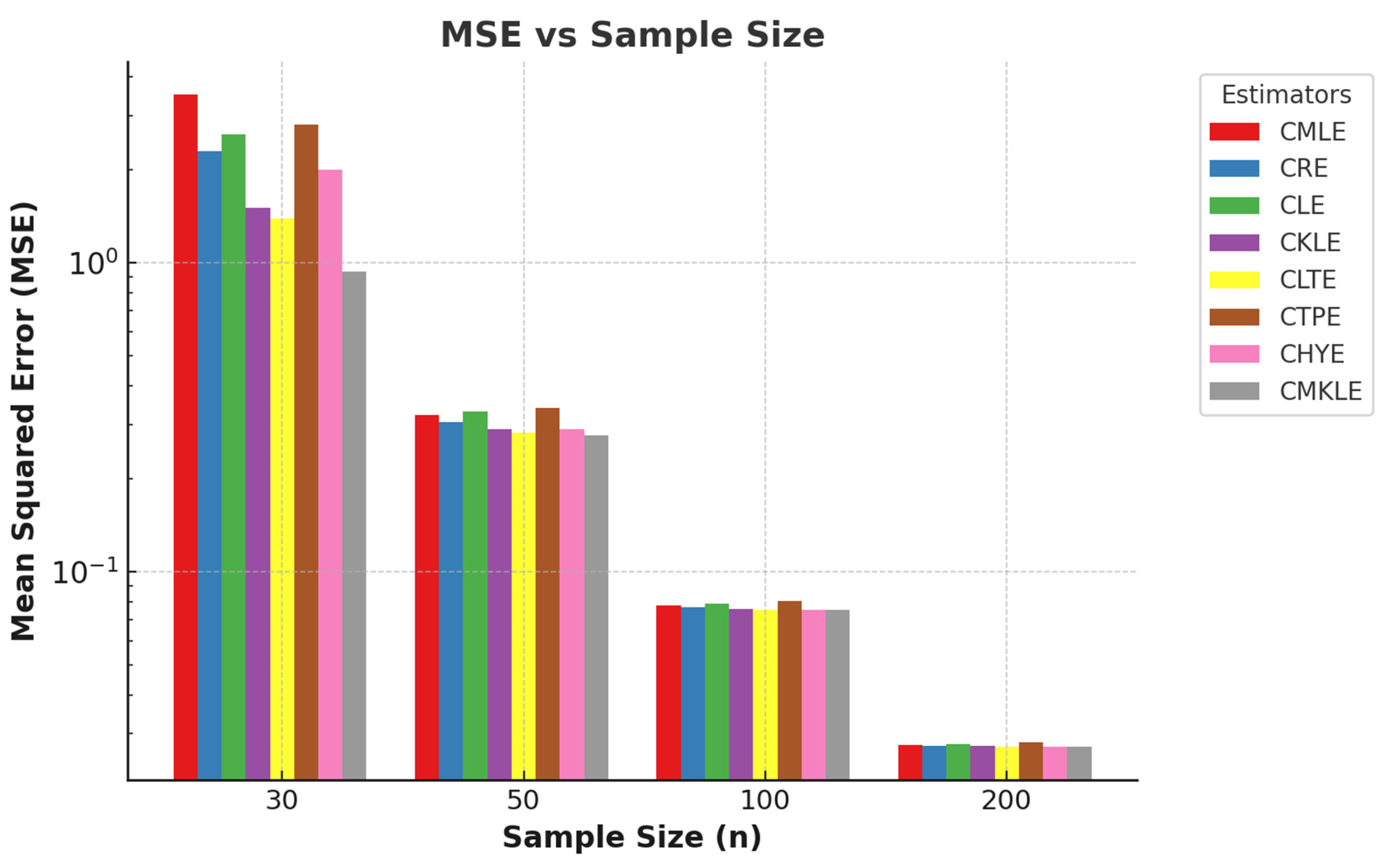
Across both tables, the MSE decreases as the sample size increases, highlighting the advantages of larger datasets. For instance, when p = 4 and $\gamma$ = 0.80, the MSE for n = 30 is relatively high (e.g., 0.4473 for the CMLE), whereas for n = 200, it drops significantly (e.g., 0.0239 for the CMLE). This trend is consistent across all levels of multicollinearity and dispersion, demonstrating that increasing the sample size reduces the estimator’s variance and improves overall performance. Conversely, small sample sizes (e.g., n = 30) lead to higher MSEs, particularly when combined with high multicollinearity (e.g., γ = 0.99) and over-dispersion. In these cases, the performance gap between estimators is most pronounced, with the proposed estimator showing more resilience to these conditions than its counterparts.

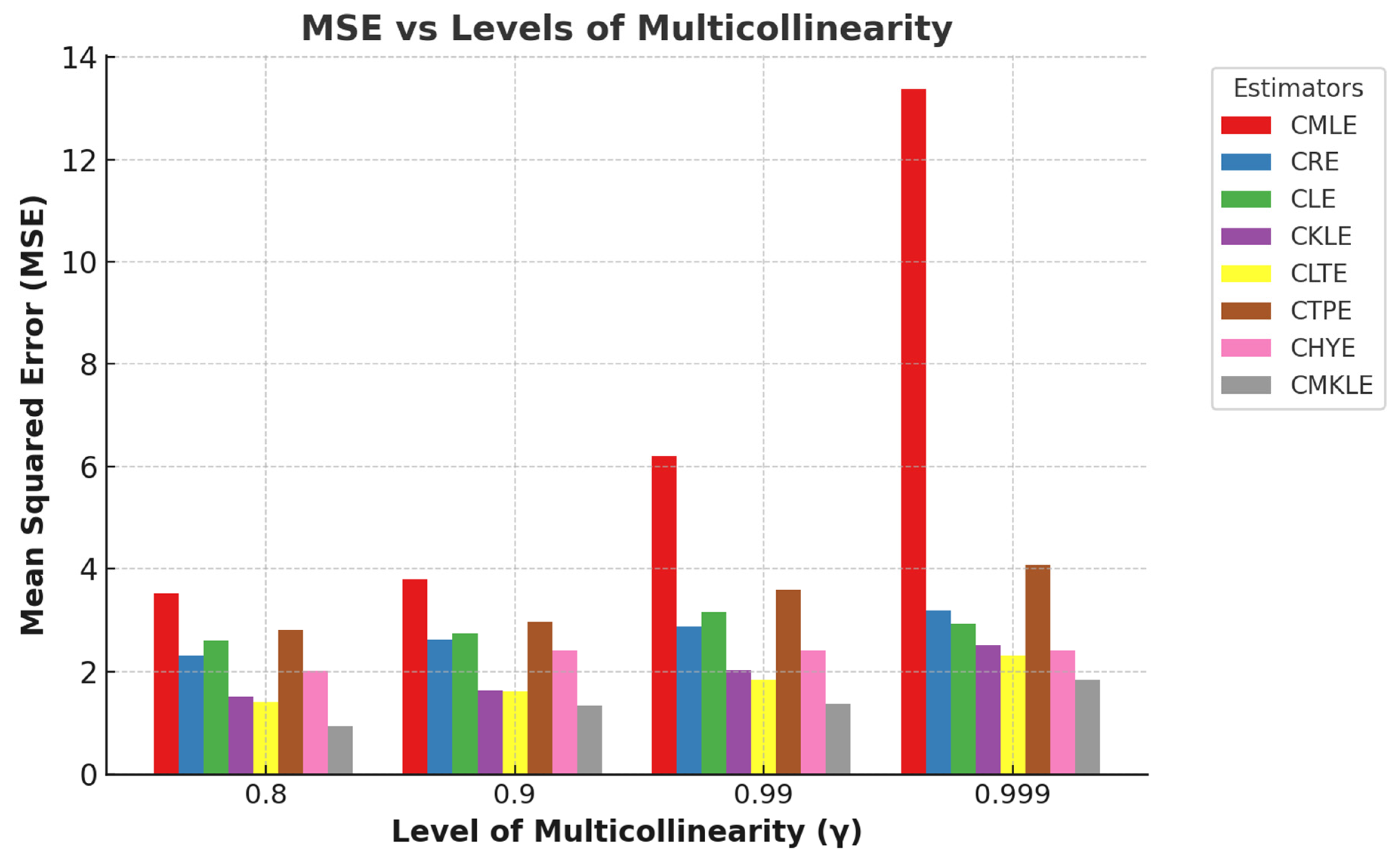
When multicollinearity is low (e.g., γ=0.8), all estimators tend to perform well, with the MSEs decreasing significantly as the sample size increases. For example, with $\nu$ = 0.9 and n = 200, the MSE values for all estimators are relatively close, indicating minimal performance differences under low correlation. However, as the correlation between predictors increases (e.g., $\gamma$ = 0.99), the MSE rises, particularly for smaller sample sizes. For instance, with p = 4 and n = 30, the MSE for the CMLE is 3.5256, reflecting poor performance under severe multicollinearity. In contrast, the proposed estimator (CMKLE) consistently shows better robustness to multicollinearity. Although the performance difference diminishes as the sample size increases, the CMKLE still maintains superior results.

Increasing the number of predictors from p = 4 (Table 1) to p = 8 (Table 2) results in higher MSE values across all conditions. For example, with $\gamma$ = 0.95 and n = 200, the MSE for p = 4 is 0.0412 (CMKLE), while for p = 8, it is 0.0470, reflecting the increased complexity in estimation with more predictors. The performance advantage of the CMKLE is more pronounced in smaller sample sizes, where it demonstrates greater robustness to both multicollinearity and dispersion effects. Even as the sample size increases and the performance gap narrows, the CMKLE maintains its leading position, reflecting its robustness and efficiency across a range of model complexities and data conditions.

Figure 1 and Figure 2, respectively, clearly illustrate the trends in the relationship between mean squared error (MSE) and sample sizes and MSE and multicollinearity levels. These figures provide compelling evidence of how variations in sample size and the degree of multicollinearity influence the predictive accuracy of the models under consideration.

5. Applications

In this study, we modeled two real-life datasets: one exhibiting over-dispersion and the other under-dispersion. By analyzing datasets with different dispersion characteristics, we aimed to demonstrate the versatility and advantages of the COM–Poisson regression model, which is uniquely capable of handling both types of dispersion. This allows for the more accurate modeling of count data compared to traditional models that are limited to addressing either over-dispersion or equi-dispersion scenarios.

5.1. Example I

In this study, we analyzed the nuts dataset, initially introduced by Hilbe [28], and most recently examined by Lukman et al. [2]. The dataset, available through the ‘COUNT’ package, comprises 52 observations and seven explanatory variables. It focuses on squirrel activity and various forest characteristics within Scotland’s Abernathy Forest. The response variable measures the number of cones stripped by squirrels per plot. In contrast, the explanatory variables include the following: the number of trees per plot ($x_1$), the number of trees with a diameter at breast height (DBH) per plot ($x_2$), mean tree height per plot ($x_3$), canopy closure percentage ($x_4$), standardized number of trees per plot ($x_5$), standardized mean tree height per plot ($x_6$), and standardized canopy closure percentage ($x_7$).

In this analysis, following Lukman et al. [2], we excluded the variable $x_5$ and $x_6$ due to the modeling difficulties they posed. Subsequent investigations revealed the presence of multicollinearity, as indicated by variance inflation factors (VIFs) of 4.474, 16.332, 39.61, and 40.89 for the remaining variables. These high VIF values suggest strong correlations between several regressors, which, combined with over-dispersion, complicate the model-fitting process. Over-dispersion was confirmed by a dispersion parameter of 13.86763, signaling that the variance far exceeds the mean. This combination of multicollinearity and over-dispersion is critical, as it can distort the estimation of regression coefficients, compromise model accuracy, and reduce the reliability of statistical inferences.

Table 3. Estimated regression coefficients for the nut dataset.

Coef.	Estimators		Lower CI	Upper CI	SMSE
$x_1$	${\widehat{\theta }}_{CMLE}$	0.0255	0.0093	0.0417	17.3187
$x_2$		2.4850	0.3523	4.6177
$x_3$		0.0367	−0.0540	0.1273
$x_4$		0.0093	−0.0103	0.0289
$x_5$		0.5178	0.0274	1.0082
$x_1$	${\widehat{\theta }}_{CRE}$	0.0192	0.0044	0.0340	3.6395
$x_2$		0.5328	0.0967	0.9688
$x_3$		0.0768	−0.0010	0.1547
$x_4$		0.0087	−0.0106	0.0280
$x_5$		0.5225	0.1237	0.9213
$x_1$	${\widehat{\theta }}_{CLE}$	0.0220	0.0150	0.0467	5.7150
$x_2$		1.3704	2.2750	6.0085
$x_3$		0.0603	−0.0863	0.0894
$x_4$		0.0087	−0.0094	0.0299
$x_5$		0.5508	−0.0204	0.9579
$x_1$	${\widehat{\theta }}_{CKLE}$	0.0129	−0.0017	0.0274	6.8430
$x_2$		−1.4194	−0.3236	0.2969
$x_3$		0.1170	0.0417	0.1923
$x_4$		0.0081	−0.0111	0.0273
$x_5$		0.5272	0.1723	0.8822
$x_1$	${\widehat{\theta }}_{CLTE}$	0.0189	0.0003	0.0295	1.4546
$x_2$		0.4364	0.1538	0.9872
$x_3$		0.0788	0.0282	0.1804
$x_4$		0.0087	−0.0109	0.0275
$x_5$		0.5228	0.1564	0.8951
$x_1$	${\widehat{\theta }}_{CTPE}$	0.0202	0.0181	0.0488	2.9229
$x_2$		0.8489	3.5568	6.2770
$x_3$		0.0703	−0.0967	0.0700
$x_4$		0.0088	−0.0096	0.0296
$x_5$		0.5218	0.2901	0.9949
$x_1$	${\widehat{\theta }}_{CHYE}$	0.0184	0.0054	0.0353	0.9609
$x_2$		0.3040	0.289	1.0766
$x_3$		0.0812	−0.0094	0.1500
$x_4$		0.0088	−0.0108	0.0281
$x_5$		0.5098	0.1019	0.9811
$x_1$	${\widehat{\theta }}_{CMKLE}$	0.0164	−0.0150	0.0105	0.8626
$x_2$		−0.2723	−0.1213	−0.2456
$x_3$		0.0902	0.1621	0.2793
$x_4$		0.0099	−0.0148	0.0235
$x_5$		0.3891	0.4309	1.1188

presents the estimated regression coefficients derived from various estimators employed in this study, which include the CMLE, CRE, CLE, CKLE, CLTE, CTPE, CHYE, and CMKLE. The performances of these estimators were evaluated using the scalar mean squared error (SMSE), as defined in Equations (32)–(39). The optimal estimator minimizes the SMSE, reflecting a lower prediction error. According to the results, the CMKLE demonstrates the lowest SMSE, with a value of 0.8626, suggesting that it provides the most precise predictions among the estimators considered in this analysis. The CHYE follows closely with an SMSE of 0.9609, also exhibiting strong performance. On the other hand, the CMLE has the highest SMSE at 17.3187, indicating that it is the least efficient estimator for this dataset.

The confidence intervals (CIs) computed for each estimator provide insights into the estimated coefficients’ statistical significance, precision, and reliability. A coefficient’s statistical significance is determined by whether its CI includes zero. If a CI does not contain zero, the coefficient is deemed statistically significant at the 5% level, indicating a meaningful contribution to the model. The CMKLE provides the most stable and precise estimates, as indicated by the lowest SMSE. However, not all coefficients are statistically significant. The results reveal that $x_2, { x}_3$ and $x_5$ are significant while $x_1$ and $x_4$ are insignificant.

In summary, the CMKLE outperforms the other methods, providing the smallest SMSE and, consequently, the best prediction accuracy. Estimators with higher SMSE values, such as the CMLE, demonstrate reduced efficiency for this dataset due to their larger prediction errors. These findings align with the simulation results presented in Table 1 and Table 2, further reinforcing the robustness of the CMKLE approach.

5.2. Example 2

The second application involves analyzing aircraft data, where the response variable represents the count of damaged locations on the aircraft, which is modeled as following a Poisson distribution [29,30]. The explanatory variables include the type of aircraft coded as 0 for A-4 and 1 for A-6 ${(x}_1)$, the bomb load in tons ($x_2$), and the total months of aircrew experience ($x_3$). Recent work by Algamal et al. [31] applied the COM–Poisson regression model for more suitable data modeling. Our analysis indicates that the dataset exhibits under-dispersion, characterized by a lower variability in counts than expected under traditional Poisson or negative binomial models. The COM–Poisson model effectively accommodates this behavior, as evidenced by the low dispersion parameter of 0.8756, which aligns with the characteristics of the dataset. Lukman et al. [4] identified significant multicollinearity issues, indicated by a condition number of 219.3654.

The results in

Table 4. Estimated regression coefficients for the aircraft data.

Coef.	Estimators		Lower CI	Upper CI	SMSE
$x_1$	${\widehat{\theta }}_{CMLE}$	0.6257	−0.2538	1.5051	0.6084
$x_2$		0.1455	0.0500	0.2410
$x_3$		−0.0166	−0.0257	−0.0076
$x_1$	${\widehat{\theta }}_{CRE}$	0.4101	−0.1587	0.9789	0.2565
$x_2$		0.1622	0.0833	0.2411
$x_3$		−0.0166	−0.0257	−0.0076
$x_1$	${\widehat{\theta }}_{CLE}$	0.7855	−0.1798	1.4106	0.5881
$x_2$		0.1331	0.0557	0.2370
$x_3$		−0.0166	−0.0257	−0.0076
$x_1$	${\widehat{\theta }}_{CKLE}$	0.1945	−0.1887	0.5777	0.0555
$x_2$		0.1789	0.1076	0.2501
$x_3$		−0.0167	−0.0257	−0.0077
$x_1$	${\widehat{\theta }}_{CLTE}$	0.2058	−0.1762	0.8525	0.1684
$x_2$		0.1780	0.0914	0.2442
$x_3$		−0.0167	−0.0257	−0.0076
$x_1$	${\widehat{\theta }}_{CTPE}$	0.9608	−0.0906	1.2988	0.5663
$x_2$		0.1196	0.0621	0.2323
$x_3$		−0.0166	−0.0257	−0.0076
$x_1$	${\widehat{\theta }}_{CHYE}$	0.5135	−0.2361	1.0430	0.2480
$x_2$		0.1543	0.0804	0.2450
$x_3$		−0.0166	−0.0257	−0.0076
$x_1$	${\widehat{\theta }}_{CMKLE}$	0.1312	−0.2520	0.5144	0.0253
$x_2$		0.1834	0.1121	0.2546
$x_3$		−0.0166	−0.0256	−0.0076

summarize the estimated regression coefficients for various estimators applied to the aircraft data, alongside the corresponding SMSE values. Among the estimators, the CMKLE demonstrates the best performance, achieving the lowest SMSE of 0.0253, indicating superior precision in coefficient estimation. The next best estimator, the CKLE, exhibits an SMSE of 0.0555, further reinforcing its reliability. In contrast, the CMLE shows relatively poorer performance, emphasizing the negative impact of multicollinearity on its performance. Given that the CMKLE outperforms other estimators in terms of having the lowest SMSE, we base our interpretation of the confidence intervals in Table 4 on the CMKLE estimates. The results from the CMKLE provide valuable insights into the relationship between the predictor variables and the response. Notably, the estimated coefficient for $x_1$ is 0.1312, with a 95% confidence interval of (−0.2520, 0.5144). Since this interval includes zero, we cannot conclude that $x_1$ has a statistically significant effect on the response variable at the given confidence level. This suggests that while $x_1$ may contribute to the model, its influence is not strong enough to be distinguished from random variation. In contrast, both $x_2$ and $x_3$ are statistically significant. The coefficient for $x_2$ is 0.1834, with a confidence interval of (0.1121, 0.2546), indicating a positive and significant relationship with the response variable. Similarly, $x_3$ has a negative coefficient of −0.0166, with a confidence interval of (−0.0256, −0.0076), confirming a significant negative effect.

Traditional estimators, such as the CMLE, may exhibit limitations in estimation accuracy, particularly in model complexities such as multicollinearity or non-normal error structures. This underscores the importance of selecting robust estimators tailored to the data’s characteristics to enhance predictive reliability. Notably, these findings align with the simulation results presented in Table 1 and Table 2, further validating the superior robustness and efficiency of the CMKLE approach.

6. Concluding Remarks

This study addresses the significant challenges posed by multicollinearity in COMP regression models by introducing a novel estimator that integrates the Kibria–Lukman and ridge estimators. This advancement significantly contributes to the existing literature, offering new methodologies that help mitigate the adverse effects of multicollinearity. Through rigorous Monte Carlo simulation studies and real-life applications using two distinct datasets, we comprehensively evaluated the performance of the proposed estimators. The simulation results reveal valuable insights into the behavior of the estimators under varying conditions, including different sample sizes, numbers of independent variables, dispersion parameters, and levels of multicollinearity. Our analysis of mean squared error (MSE) values across these variables demonstrated a consistent pattern: MSE values were generally lower under conditions of under-dispersion (ν = 0.9) compared to over-dispersion (ν = 1.25), particularly as sample sizes increased. The best-performing estimators exhibited significantly lower MSEs with larger sample sizes and reduced multicollinearity, underscoring their robustness.

Moreover, our findings emphasize the benefits of larger datasets, where the MSE consistently decreased with increasing sample size. This trend highlights the critical importance of sufficient sample sizes in enhancing estimator performance, particularly when there is high multicollinearity and over-dispersion. Conversely, smaller sample sizes resulted in high MSEs, illustrating the pronounced performance gap among estimators under these challenging conditions. Notably, the proposed CMKLE demonstrated superior resilience to multicollinearity, maintaining outstanding performance even as sample sizes increased. As we increased the number of predictors from p = 4 to p = 8, we observed a corresponding increase in MSE values across all conditions, confirming the complexities introduced by additional predictors. Notably, the CMKLE displayed a pronounced advantage in smaller sample sizes, demonstrating its robustness against multicollinearity and dispersion effects.

Furthermore, the application results reinforced the superior performance of the CMKLE. The scalar mean squared error (SMSE) evaluations indicate that the CMKLE achieved the lowest SMSE, demonstrating the highest predictive accuracy among the estimators analyzed. In contrast, the traditional CMLE displayed significantly higher SMSE values, highlighting its reduced efficiency for this dataset. In conclusion, the CMKLE surpasses other methodologies in predictive accuracy but also underscores the necessity for careful selection of estimation techniques tailored to specific data characteristics. This research paves the way for future studies to explore the broader application of these methodologies across diverse fields, ultimately enhancing the robustness of statistical models in the presence of multicollinearity and varying dispersion conditions.

Additionally, future research could explore Bayesian approaches to COM–Poisson regression, which have been proposed in the literature as an alternative methodology for handling dispersed count data. Bayesian inference methods, such as those developed by Chanialidis et al. [32], offer flexible estimation techniques that may provide further improvements in model performance and computational efficiency.

References

1. Francis, R.A.; Geedipally, S.R.; Guikema, S.D.; Dhavala, S.S.; Lord, D.; LaRocca, S. Characterizing the performance of the conway-maxwell Poisson generalized linear model. Risk Anal. Int. J. 2012, 32, 167–183. [Google Scholar] [CrossRef] [PubMed]
2. Lukman, A.F.; Albalawi, O.; Arashi, M.; Allohibi, J.; Alharbi, A.A.; Farghali, R.A. Robust Negative Binomial Regression via the Kibria–Lukman Strategy: Methodology and Application. Mathematics 2024, 12, 2929. [Google Scholar] [CrossRef]
3. Walters, G.D. Using Poisson class regression to analyze count data in correctional and forensic psychology: A relatively old solution to a relatively new problem. Crim. Justice Behav. 2007, 34, 1659–1674. [Google Scholar] [CrossRef]
4. Lukman, A.F.; Adewuyi, E.; Månsson, K.; Kibria, B.G. A new estimator for the multicollinear Poisson regression model: Simulation and application. Sci. Rep. 2021, 11, 3732. [Google Scholar] [CrossRef]
5. Månsson, K. On ridge estimators for the negative binomial regression model. Econ. Model. 2012, 29, 178–184. [Google Scholar] [CrossRef]
6. Conway, R.W.; Maxwell, W.L. A queuing model with state dependent service rates. J. Ind. Eng. Int. 1962, 12, 132–136. [Google Scholar]
7. Chatla, S.B.; Shmueli, G. Efficient estimation of COM–Poisson regression and a generalized additive model. Comput. Stat. Data Anal. 2018, 121, 71–88. [Google Scholar] [CrossRef]
8. Abonazel, M.R.; Saber, A.A.; Awwad, F.A. Kibria–Lukman estimator for the Conway–Maxwell Poisson regression model: Simulation and applications. Sci. Afr. 2023, 19, e01553. [Google Scholar] [CrossRef]
9. Tanış, C.; Asar, Y. Liu-type estimator in Conway–Maxwell–Poisson regression model: Theory, simulation and application. Statistics 2024, 58, 65–86. [Google Scholar] [CrossRef]
10. Abonazel, M.R. New modified two-parameter Liu estimator for the Conway–Maxwell Poisson regression model. J. Stat. Comput. Simul. 2023, 93, 1976–1996. [Google Scholar] [CrossRef]
11. Sami, F.; Amin, M.; Butt, M.M. On the ridge estimation of the Conway-Maxwell Poisson regression model with multicollinearity: Methods and applications. Concurr. Comput. Pract. Exp. 2022, 34, e6477. [Google Scholar] [CrossRef]
12. Akram, M.N.; Amin, M.; Sami, F.; Mastor, A.B.; Egeh, O.M.; Muse, A.H. A new Conway Maxwell–Poisson Liu regression estimator—Method and application. J. Math. 2022, 2022, 3323955. [Google Scholar] [CrossRef]
13. Aladeitan, B.B.; Adebimpe, O.; Lukman, A.F.; Oludoun, O.; Abiodun, O.E. Modified Kibria-Lukman (MKL) estimator for the Poisson Regression Model: Application and simulation. F1000Research 2021, 10, 548. [Google Scholar] [CrossRef]
14. Sellers, K.F.; Shmueli, G. A flexible regression model for count data. Ann. Appl. Stat. 2010, 4, 943–961. [Google Scholar] [CrossRef]
15. Hoerl, A.E.; Kennard, R.W. Ridge regression: Biased estimation for nonorthogonal problems. Technometrics 1970, 12, 55–67. [Google Scholar] [CrossRef]
16. Liu, K. A new class of blased estimate in linear regression. Commun. Stat. Theory Methods 1993, 22, 393–402. [Google Scholar]
17. Liu, K. Using Liu-type estimator to combat collinearity. Commun. Stat. Theory Methods 2003, 32, 1009–1020. [Google Scholar] [CrossRef]
18. Kibria, B.G.; Lukman, A.F. A new ridge-type estimator for the linear regression model: Simulations and applications. Scientifica 2020, 2020, 9758378. [Google Scholar] [CrossRef] [PubMed]
19. Özkale, M.R.; Kaciranlar, S. The restricted and unrestricted two-parameter estimators. Commun. Stat. Theory Methods 2007, 36, 2707–2725. [Google Scholar] [CrossRef]
20. Sakallıoğlu, S.; Kaçıranlar, S. A new biased estimator based on ridge estimation. Stat. Pap. 2008, 49, 669–689. [Google Scholar] [CrossRef]
21. Asar, Y.; Genç, A. A new two-parameter estimator for the Poisson regression model. Iran. J. Sci. Technol. Trans. A Sci. 2018, 42, 793–803. [Google Scholar] [CrossRef]
22. Huang, J.; Yang, H. A two-parameter estimator in the negative binomial regression model. J. Stat. Comput. Simul. 2014, 84, 124–134. [Google Scholar] [CrossRef]
23. Sami, F.; Butt, M.M.; Amin, M. Two parameter estimators for the Conway–Maxwell–Poisson regression model. J. Stat. Comput. Simul. 2023, 93, 2137–2157. [Google Scholar] [CrossRef]
24. Kibria, B.G. Performance of some new ridge regression estimators. Commun. Stat. -Simul. Comput. 2003, 32, 419–435. [Google Scholar] [CrossRef]
25. Oranye, H.E.; Ugwuowo, F.I. Modified jackknife Kibria–Lukman estimator for the Poisson regression model. Concurr. Comput. Pract. Exp. 2022, 34, e6757. [Google Scholar] [CrossRef]
26. Sellers, K.; Lotze, T.; Raim, A. Compoissonreg: Conway-Maxwell Poisson (Com-Poisson) Regression; R Package Version 0.4; The Comprehensive R Archive Network: Vienna, Austria, 2017; Volume 1. [Google Scholar]
27. Sellers, K.F.; Raim, A. A flexible zero-inflated model to address data dispersion. Comput. Stat. Data Anal. 2016, 99, 68–80. [Google Scholar] [CrossRef]
28. Hilbe, J.M. Negative Binomial Regression, 2nd ed.; Cambridge University Press: Cambridge, UK, 2011. [Google Scholar]
29. Myers, R.H.; Montgomery, D.C.; Vining, G.; Robinson, T.J. Generalized Linear Models: With Applications in Engineering and the Sciences; John Wiley & Sons: Hoboken, NJ, USA, 2012. [Google Scholar]
30. Amin, M.; Akram, M.N.; Amanullah, M. On the James-Stein estimator for the Poisson regression model. Commun. Stat.-Simul. Comput. 2022, 51, 5596–5608. [Google Scholar] [CrossRef]
31. Algamal, Z.Y.; Abonazel, M.R.; Awwad, F.A.; Eldin, E.T. Modified jackknife ridge estimator for the Conway-Maxwell-Poisson model. Sci. Afr. 2023, 19, e01543. [Google Scholar] [CrossRef]
32. Chanialidis, C.; Evers, L.; Neocleous, T.; Nobile, A. Efficient Bayesian inference for COM-Poisson regression models. Stat. Comput. 2018, 28, 595–608. [Google Scholar] [CrossRef]
Figure 1. A sample plot of the sample size against the mean squared error.
Mathematics 13 00794 g001
Figure 2. A sample plot of the mean squared error against the level of multicollinearity.
Mathematics 13 00794 g002