Inference and Optimal Design on Partially Accelerated Life Tests for the Power Half-Logistic Distribution Under Adaptive Type II Progressive Censoring

Abstract

This study explores accelerated life tests to examine the durability of highly reliable products. These tests involve applying higher stress levels, such as increased temperature, voltage, or pressure, that cause early failures. The power half-logistic (PHL) distribution is utilized due to its flexibility in modeling the probability density and hazard rate functions, effectively representing various data patterns commonly encountered in practical applications. The step stress partially accelerated life testing model is analyzed under an adaptive type II progressive censoring scheme, with samples drawn from the PHL distribution. The maximum likelihood method estimates model parameters and calculates asymptotic confidence intervals. Bayesian estimates are also obtained using Lindley’s approximation and the Markov Chain Monte Carlo (MCMC) method under different loss functions. Additionally, D- and A-optimality criteria are applied to determine the optimal stress-changing time. Simulation studies are conducted to evaluate the performance of the estimation methods and the optimality criteria. Finally, real-world datasets are analyzed to demonstrate the practical usefulness of the proposed model.

1. Introduction

Manufacturers are designing and producing more reliable products as a result of today’s heightened consumer demands and growing market competition. With a decreasing time-to-market, it is critical to evaluate and estimate the product’s reliability during the design and development phase. In addition, due to technological advancements, production designs are always changing. Therefore, it is becoming more difficult to find information regarding the lifespan of goods or materials that are highly reliable when tested under normal conditions. To address this, the industrial sector often uses accelerated life testing (ALT) or partially accelerated life testing (PALT) to quickly gather sufficient failure data and understand the relationship between failures and external stress factors. These tests can significantly save time, labor, resources, and costs.

In ALTs, all units are subjected to stress levels higher than usual to induce failures more quickly. In contrast, PALTs involve testing units under both normal and elevated stress conditions intended to collect more failure data within a constrained time frame without subjecting all units to high stress. PALTs are particularly beneficial in scenarios where time and cost are pressing concerns. The information obtained from such tests can be utilized to estimate the failure behavior of the units under normal conditions. DeGroot and Goel performed a proper statistical modeling of PALTs [1], where the authors considered the tempered random variable model for PALTs.

Nelson [2] suggested various methods to apply stress under accelerated testing conditions, with constant stress and step stress models being the most widely used. In a step stress partially accelerated life test (SSPALT), units are exposed to progressively higher stress levels either at predetermined times or until a specified number of failures occur. This type of test often involves two stress levels, starting with a normal stress level and transitioning to a higher level after a fixed duration. Additional details about step stress accelerated life testing can be found in [3]. Several researchers have studied SSPALT, including [4,5,6,7,8].

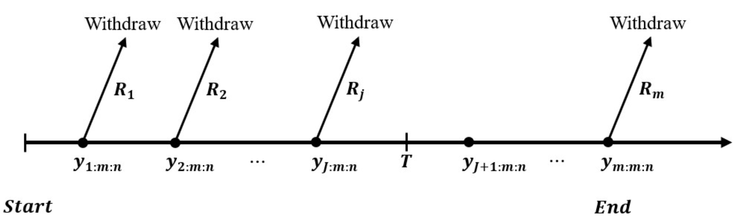
The censoring data are of natural interest in survival, reliability, and medical studies due to cost or time considerations. Although traditional type I and type II censoring methods are widely used, progressive censoring schemes (type I and type II) offer significant advances in data collection in lifetime studies. These progressive schemes address the limitations in the flexibility of conventional methods. The type II progressive censoring (TIIPC) scheme, specifically, generalizes the traditional type II approach by allowing for the removal of units throughout the experiment, not just at the endpoint. In the TIIPC scheme, n units are placed in a test. Let $y_i,i=1,2,\dots ,m$ denote the times at which the $i^{th}$ failure is recorded for m of the n units. Immediately after the first failure $y_{1:m:n}$, $R_1$ units are randomly removed from the surviving units. At the time $X_{2:m:n}$ of the second failure, $R_2$ units of the remaining $n-2-R_1$ surviving units are randomly eliminated, and so on. The test continues until the failure time $m^{th}$$y_{m:m:n}$. The experiment ends and the remaining $R_m=n-m-{\sum }_{i=1}^{m-1}{R}_i$ surviving units are eliminated. Removals $R_1,R_2,\dots ,R_m$ are predetermined in such a way that $m+{\sum }_{i=1}^{m-1}{R}_i=n$. References [9,10] discussed the advantages of the TIIPC schemes.

The TIIPC scheme offers flexibility in the design of an experiment by allowing for predetermined removal times ($R_1,R_2,\dots ,R_m$) of units during the test. However, a crucial limitation of TIIPC is the unknown and potentially lengthy operating time (T) compared to traditional type II censoring, as highlighted in [11]. This extended time frame may not be preferable in practical applications due to time constraints or unexpected developments. Consequently, ref. [11] proposed adaptive type II progressive censoring (ATIIPC) to allow experimenters to adjust the planned removal schedule of the surviving units during the test. Recently, interest has been paid to studying SSPALT models under the ATIIPC scheme, including [12,13,14,15,16].

Statistical analysis and modeling of lifetime data play a vital role in various applied sciences, including engineering, economics, insurance, and biological sciences. To address these needs, numerous continuous distributions have been proposed in the statistical literature, such as exponential, Lindley, gamma, log-normal, half-logistic, and Weibull distributions. Among these, the power half-logistic (PHL) distribution has been extensively utilized to analyze lifetime and reliability data. The PHL distribution, introduced by Krishnarani [17], is defined as follows:

Let X be a random variable following the half-logistic distribution with a survival function:

$$\overline{G}(x;\beta )={\displaystyle \frac{2}{1+e^{\beta x}}},\beta ,x>0.$$

(1)

Consider the transformation $Y=X^{1/\alpha }$, then the distribution of Y follows the PHL distribution, which is characterized by a scale parameter $\beta$ and a shape parameter $\alpha$. Its probability density function (pdf), survival function $S\left(y\right)$, and hazard rate function (hf) are defined as follows:

$$f(y;\alpha ,\beta )={\displaystyle \frac{2\alpha \beta e^{\beta y^{\alpha }}{y}^{\alpha -1}}{{(1+e^{\beta y^{\alpha }})}^2}},$$

(2)

$$S(y;\alpha ,\beta )={\displaystyle \frac{2}{(1+e^{\beta y^{\alpha }})}},$$

(3)

and

$$h(y;\alpha ,\beta )={\displaystyle \frac{\alpha \beta e^{\beta y^{\alpha }}{y}^{\alpha -1}}{(1+e^{\beta y^{\alpha }})}},$$

(4)

where $\alpha ,\beta ,y>0$, and the cumulative distribution function (cdf) is $F(y;\alpha ,\beta )=1-S(y;\alpha ,\beta )$.

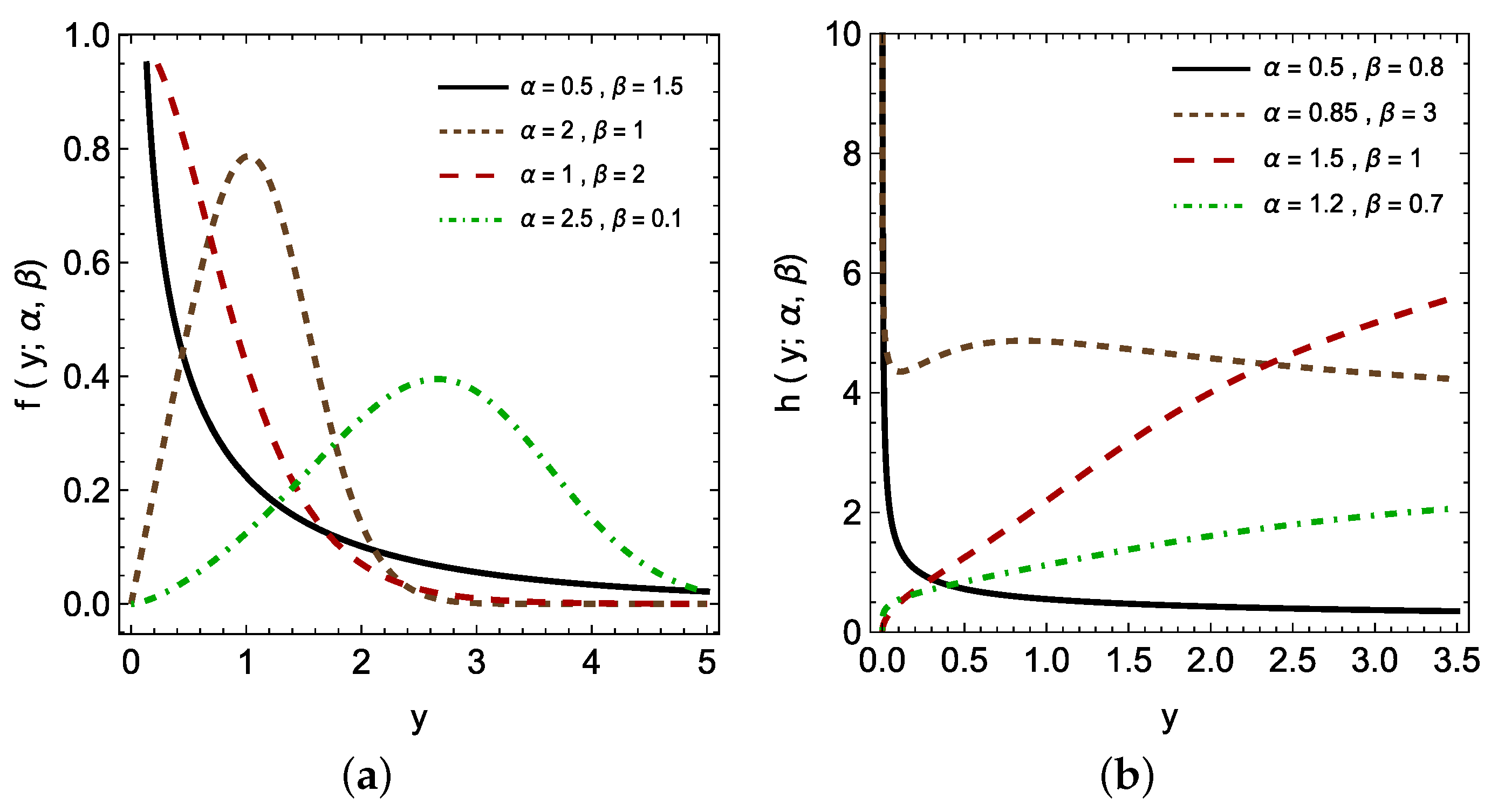
The PHL distribution is a versatile model capable of capturing a wide range of lifetime data, including symmetric and asymmetric types. Its flexibility allows us to represent various data patterns commonly encountered in practical applications effectively. To illustrate the PHL flexibility, Figure 1 shows the plots of the pdf and the hazard rate function for different values of the parameters $\alpha$ and $\beta$. The PHL distribution has found successful applications in various fields. For example, Alomani et al. [18] demonstrate the flexibility of the PHL distribution in modeling a wide range of datasets, including COVID-19 [19], time between failures of secondary reactor pumps [20], and active repair times for 40 airborne communication transceivers [21]. Additionally, Alomani et al. [18] addressed various estimation techniques and data analysis methods for constant-partially accelerated life tests for the PHL distribution. El-Awady et al. [22] further extend this work by investigating the properties and parameter estimation of a generalized form of the PHL distribution, known as the Exponentiated Half-Logistic Weibull (EHLW) distribution. They also examine the stress strength reliability parameter ( $P(X>Y)$ ) within the context of the EHLW distribution.

This study is motivated by the growing need for robust statistical modeling techniques in reliability and life testing, particularly under complex experimental conditions such as the SSPALT and ATIIPC schemes. These scenarios are highly relevant in engineering and industrial applications, where understanding the reliability of components under varying stress levels is essential. The ATIIPC scheme, in particular, offers enhanced flexibility by allowing experimenters to adapt the the removal schedule of units during the test, making it well suited for real-world applications with time and resource constraints.

As the PHL distribution has proven to provide significant flexibility in modeling a wide range of lifetime data, including symmetric and asymmetric failure patterns, particularly in reliability analysis under accelerated testing conditions, there remains a critical gap in the literature regarding the application of the PHL distribution under complex experimental conditions such as the SSPALT and ATIIPC schemes. This study addresses this gap by focusing on estimating the parameters of the PHL distribution and the acceleration parameter when the data are derived from the ATIIPC scheme under the SSPALT model.

To achieve this, both maximum likelihood estimation (MLE) and Bayesian methods are employed. MLE is utilized for its well-established theoretical properties, such as consistency and asymptotic efficiency, which make it a standard choice for parameter estimation in reliability studies. For the Bayesian inference, Lindley’s approximation and Markov Chain Monte Carlo (MCMC) techniques are used. Lindley’s approximation provides approximate Bayesian estimates when closed-form solutions are unavailable, leveraging its computational simplicity and efficiency for initial parameter estimation. MCMC, on the other hand, is a powerful and flexible technique for sampling from complex posterior distributions, especially in high-dimensional parameter spaces. It provides accurate and robust estimates by converging to the true posterior distribution, even for small sample sizes. Furthermore, this study explores the problem of determining the optimal stress change time using two distinct optimality criteria.

The structure of this paper is organized as follows. Section 2 introduces the SSPALT model under the ATIIPC scheme using the PHL distribution. Section 3 provides maximum likelihood estimates (MLEs) and asymptotic confidence intervals (ACIs). In Section 4, we discuss the derivation of Bayesian estimates using Lindley’s approximation and the Markov Chain Monte Carlo (MCMC) technique. Section 5 examines two optimality criteria to determine the optimal timing for changing the stress level. Section 6 presents Monte Carlo simulation studies to showcase the effectiveness of the point and interval estimates for the parameters, as well as the optimal time for altering the stress level. Section 7 details the data analysis conducted for specific case studies. Finally, Section 8 concludes the paper with a summary of the findings.

2. Model Assumptions

In the ATIIPC scheme, an initial estimate for the experiment duration, $T>0$, is set, which can be surpassed if necessary. The desired number of failures (m) is specified. Furthermore, censoring schemes ($R_i\ge 0$, $i=1,2,\dots ,m$) are predetermined, but these $R_i$ values can be adapted during the experiment. The ATIIPC scheme balances reducing experiment time with acquiring sufficient data (including extreme lifetimes) for robust statistical inference. This is achieved through a dynamic termination strategy based on two cases:

Case (i):

If $T\ge Y_{m:m:n}$, all m failures are observed, and the experiment ends at the predetermined time (T). The preassigned censoring scheme ($R_1,R_2,\dots ,R_m$) is followed.

Case (i):

If $T<Y_{m:m:n}$, the experiment continues beyond the planned duration T. Suppose J failures have occurred such that $Y_{J:m:n}<T<Y_{J+1:m:n}$, where $0\le J\le m-1$ and $Y_{0:m:n}=0$. In this scenario, the test is immediately terminated with the $m_{th}$ failure. Consequently, the censoring scheme ($R_i$) is dynamically adjusted to become $(R_1,R_2,\dots ,R_J,0,\dots ,0,R_m^{*})$, where $R_m^{*}=n-m-{\sum }_{i=1}^{m-1}{R}_i$. Figure 2 and Figure 3 illustrate the two cases of the ATIIPC schemes.

Under SSPALT, the lifetime of the unit is given as follows:

$$Y=\left\{\begin{array}{cc}Z,\hfill & Z<\tau ,\hfill \\ \tau +{\displaystyle \frac{Z-\tau }{\gamma }},\hfill & Z>\tau .\hfill \end{array}\right.$$

where Z is the lifetime of the unit under normal use conditions, $\tau$ is the stress change time, $\gamma >1$ is the acceleration factor, and Y is the total lifetime under SSPALT. The above variable transformation is proposed by [1]. The pdf of Y under the SSPALT model can be expressed as

$$f\left(y\right)=\left\{\begin{array}{cc}0\hfill & \mathrm{if}y<0\hfill \\ f_l\left(y\right)\equiv f(y;\alpha ,\beta )\hfill & \mathrm{if}0<y<\tau \hfill \\ f_u\left(y\right)\hfill & \mathrm{if}y>\tau \hfill \end{array}\right.,$$

where $f(y;\alpha ,\beta )$ is the pdf of the PHL distribution defined in Equation (2) with the corresponding survival function given in Equation (3), and $f_u\left(y\right)$ is given by

$$f_u\left(y\right)=\gamma f_l(\tau +\gamma (y-\tau ))={\displaystyle \frac{2\alpha \beta \gamma e^{\beta {(\tau +\gamma (y-\tau ))}^{\alpha }}{(\tau +\gamma (y-\tau \left)\right)}^{\alpha -1}}{{(1+e^{\beta {(\tau +\gamma (y-\tau ))}^{\alpha }})}^2}},$$

(5)

where $\alpha ,\beta >0,\gamma >1,$ and $y>\tau$. The corresponding survival function is

$$S_u\left(y\right)={\displaystyle \frac{2}{1+e^{\beta {(\tau +\gamma (y-\tau ))}^{\alpha }}}},\alpha ,\beta >0,\gamma >1,y>\tau .$$

(6)

Figure 2. The test time $T\ge y_{m:m:n}$.

Figure 2. The test time $T\ge y_{m:m:n}$.

Figure 3. The test time $T<y_{m:m:n}$.

Figure 3. The test time $T<y_{m:m:n}$.

Under SSPALT with the ATIIPC scheme, n units undergo testing with a progressive censoring scheme $(R_1,R_2,\dots ,R_m)$. Each unit operates under normal conditions and if it does not fail up to time $\tau$, it is subjected to accelerated conditions. The experiment continues until censoring time T. In this scenario, no items are withdrawn except at the time of the $m_{th}$ failure, when all remaining surviving units are removed. The applied scheme in this case is $(R_1,\dots ,R_J,0,\dots ,0,R_m^{*})$, and the observed data take the form

$$y_{1:m:n}<\cdots <y_{m_l:m:n}\le \tau <y_{m_l+1:m:n}<\cdots <y_{J:m:n}<T<y_{J+1:m:n}<\cdots <y_{m:m:n}.$$

If $T\to 0$, the ATIIPC scheme reduces to the traditional type II censoring scheme. If $T\to \infty$, the ATIIPC scheme will lead us to the conventional TIIPC scheme.

The statistical inference based on the ATIIPC scheme under SSPALT will be described in the following sections.

3. Maximum Likelihood Estimation

Based on the ATIIPC scheme, the likelihood function of the parameter vector $\theta =(\alpha ,\beta ,\gamma )$ is provided by

$$L(\alpha ,\beta ,\gamma )={\left(2\alpha \beta \right)}^m{\gamma }^{m_u}\prod _{i=1}^{m_l}{2}^{R_i}{e}^{\beta y_i^{\alpha }}{y}_i^{\alpha -1}{u}_i^{-(R_i+2)}\prod _{i=m_l+1}^m{e}^{\beta z_i^{\alpha }}{z}_i^{\alpha -1}{v}_i^{-2}\prod _{i=m_l+1}^J{\left({\displaystyle \frac{2}{v_i}}\right)}^{R_i}{\left({\displaystyle \frac{2}{v_m}}\right)}^{D_J},$$

(7)

where $y_i=y_{i:m:n}$, $D_j=n-m-{\sum }_{i=1}^J{R}_i$, $m_u=m-m_l$, $u_i=1+e^{\beta y_i^{\alpha }}$, $z_i=(\tau +\gamma (y_i-\tau ))$, $z_m=(\tau +\gamma (y_m-\tau ))$, $v_i=1+e^{\beta {(\tau +\gamma (y_i-\tau ))}^{\alpha }}$ and $v_m=1+e^{\beta {(\tau +\gamma (y_m-\tau ))}^{\alpha }}$.

The MLE is a popular method for estimating unknown parameters because it produces accurate and statistically sound results. Apply the natural logarithm to both sides of Equation (7).

$$\begin{array}{cc}\hfill \ell (\alpha ,\beta ,\gamma )=& mlog\left(2\alpha \beta \right)+\beta \sum _{i=1}^{m_l}{y}_i^{\alpha }+(\alpha -1)\sum _{i=1}^{m_l}log{y}_i-2\sum _{i=1}^{m_l}log{u}_i+\sum _{i=1}^{m_l}{R}_{i}log\left(2u_i^{-1}\right)-2\sum _{i=m_l+1}^{m}log{v}_i\hfill \\ \hfill & +m_{u}log\left(\gamma \right)+\beta \sum _{i=m_l+1}^m{z}_i^{\alpha }+(\alpha -1)\sum _{i=m_l+1}^{m}log{z}_i+\sum _{i=m_l+1}^J{R}_{i}log\left(2v_i^{-1}\right)+D_{J}log\left(2v_m^{-1}\right)\hfill \end{array}$$

(8)

To obtain the MLEs of the parameters $\alpha ,\beta$, and $\gamma$, solve the following system of nonlinear equations.

$$\begin{array}{c}\hfill {\displaystyle \frac{\partial \ell }{\partial \alpha }}={\displaystyle \frac{m}{\alpha }}+\sum _{i=1}^{m_l}log\left(y_i\right)\left[1+\beta y_i^{\alpha }\right]-\sum _{i=1}^{m_l}(R_i+2)A_i+\sum _{i=m_l+1}^{m}log\left(z_i\right)\left[1+\beta z_i^{\alpha }\right]-2\sum _{i=m_l+1}^m{B}_i-\sum _{i=m_l+1}^J{B}_i{R}_i-D_J{B}_m\end{array}$$

(9)

$${\displaystyle \frac{\partial \ell }{\partial \beta }}={\displaystyle \frac{m}{\beta }}+\beta \sum _{i=1}^{m_l}{y}_i^{\alpha }-\sum _{i=1}^{m_l}(R_i+2){\displaystyle \frac{y_i^{\alpha }{e}^{\beta y_i^{\alpha }}}{u_i}}+\sum _{i=m_l+1}^m{z}_i^{\alpha }-2\sum _{i=m_l+1}^m{\displaystyle \frac{z_i^{\alpha }{e}^{\beta z_i^{\alpha }}}{v_i}}-\sum _{i=m_l+1}^J{R}_i{\displaystyle \frac{z_i^{\alpha }{e}^{\beta z_i^{\alpha }}}{v_i}}-D_j{\displaystyle \frac{z_m^{\alpha }{e}^{\beta z_m^{\alpha }}}{v_m}}$$

(10)

and

$$\begin{array}{cc}\hfill {\displaystyle \frac{\partial \ell }{\partial \gamma }}& ={\displaystyle \frac{m_u}{\gamma }}+\alpha \beta \sum _{i=m_l+1}^m(y_i-\tau )z_i^{\alpha -1}+(\alpha -1)\sum _{i=m_l+1}^m{\displaystyle \frac{(y_i-\tau )}{z_i}}-2\alpha \beta \sum _{i=m_l+1}^m{\displaystyle \frac{(y_i-\tau )z_i^{\alpha -1}{e}^{\beta z_i^{\alpha }}}{v_i}}\hfill \\ \hfill & -\alpha \beta \sum _{i=m_l+1}^J{R}_i{\displaystyle \frac{(y_i-\tau )z_i^{\alpha -1}{e}^{\beta z_i^{\alpha }}}{v_i}}-\alpha \beta D_j{\displaystyle \frac{(y_m-\tau )z_m^{\alpha -1}{e}^{\beta z_m^{\alpha }}}{v_m}},\hfill \end{array}$$

(11)

where $A_i={\displaystyle \frac{\beta log\left[y_i\right]y_i^{\alpha }{e}^{\beta y_i^{\alpha }}}{u_i}}$, $B_i={\displaystyle \frac{\beta log\left[z_i\right]z_i^{\alpha }{e}^{\beta z_i^{\alpha }}}{v_i}}$ and $B_m={\displaystyle \frac{\beta log\left[z_m\right]z_m^{\alpha }{e}^{\beta z_m^{\alpha }}}{v_m}}$. Obtaining closed-form solutions for the parameters in the nonlinear equations mentioned above is complicated. We use an iterative strategy, like Newton–Raphson, to obtain numerical solutions for nonlinear systems.

Approximate Confidence Intervals

The large-sample property of the MLEs suggests that, under regularity conditions, the MLEs of the parameters $\alpha$, $\beta$, and $\gamma$ are asymptotically normally distributed. To be more specific, $[(\widehat{\alpha }-\alpha ),(\widehat{\beta }-\beta ),(\widehat{\gamma }-\gamma )]\sim N(0,\Sigma )$ is known to provide the asymptotic distribution of the MLEs of $\alpha ,\beta$, and $\gamma$, where $\Sigma$ represents the variance–covariance matrix. The inverse of the Fisher Information Matrix (FIM), denoted $I^{-1}$, provides an estimate of $\Sigma$. The FIM is derived by taking the expected values of the negative second-order partial derivatives of the log-likelihood function with respect to the parameters $\alpha ,\beta$, and $\gamma$:

$$\begin{array}{c}\hfill I=-E\left[\begin{array}{ccc}{\displaystyle \frac{{\partial }^2\ell }{\partial {\alpha }^2}}& {\displaystyle \frac{{\partial }^2\ell }{\partial \alpha \partial \beta }}& {\displaystyle \frac{{\partial }^2\ell }{\partial \alpha \partial \gamma }}\\ \\ {\displaystyle \frac{{\partial }^2\ell }{\partial \beta \partial \alpha }}& {\displaystyle \frac{{\partial }^2\ell }{\partial {\beta }^2}}& {\displaystyle \frac{{\partial }^2\ell }{\partial \beta \partial \gamma }}\\ \\ {\displaystyle \frac{{\partial }^2\ell }{\partial \gamma \partial \alpha }}& {\displaystyle \frac{{\partial }^2\ell }{\partial \gamma \partial \beta }}& {\displaystyle \frac{{\partial }^2\ell }{\partial {\gamma }^2}}\end{array}\right].\end{array}$$

(12)

In practice, due to the complexity of the pdf and the integral expressions involved, the observed FIM is often used as an approximation. The observed FIM is computed using the MLEs $\widehat{\alpha }$, $\widehat{\beta }$, and $\widehat{\gamma }$:

$$\begin{array}{c}\hfill \mathbb{O}={\left[\begin{array}{ccc}-{\displaystyle \frac{{\partial }^2\ell }{\partial {\alpha }^2}}& -{\displaystyle \frac{{\partial }^2\ell }{\partial \alpha \partial \beta }}& -{\displaystyle \frac{{\partial }^2\ell }{\partial \alpha \partial \gamma }}\\ \\ -{\displaystyle \frac{{\partial }^2\ell }{\partial \beta \partial \alpha }}& -{\displaystyle \frac{{\partial }^2\ell }{\partial {\beta }^2}}& -{\displaystyle \frac{{\partial }^2\ell }{\partial \beta \partial \gamma }}\\ \\ -{\displaystyle \frac{{\partial }^2\ell }{\partial \gamma \partial \alpha }}& -{\displaystyle \frac{{\partial }^2\ell }{\partial \gamma \partial \beta }}& -{\displaystyle \frac{{\partial }^2\ell }{\partial {\gamma }^2}}\end{array}\right]}_{|\alpha =\widehat{\alpha },\beta =\widehat{\beta },\gamma =\widehat{\gamma }}\end{array}$$

(13)

where

$$\begin{array}{cc}\hfill {\displaystyle \frac{{\partial }^2\ell }{\partial {\alpha }^2}}& ={\displaystyle \frac{-m}{{\alpha }^2}}-D_j{B}_m\left[log\left[z_m\right]-B_m+\beta z_m^{\alpha }log\left[z_m\right]\right]+\beta \sum _{i=1}^{m_l}{y}_i^{\alpha }log{\left[y_i\right]}^2+\sum _{i=1}^{m_l}{A}_i(R_i+2)(log\left[y_i\right]+A_i+\beta log\left[y_i\right]y_i^{\alpha })\hfill \\ \hfill & +\beta \sum _{i=m_l+1}^m{z}_i^{m}log{\left[z_i\right]}^2-2\sum _{i=m_l+1}^m{B}_i[log\left[z_i\right]-B_i\beta log\left[z_i\right]z_i^{\alpha }]+\sum _{i=m_l+1}^J{R}_i{B}_i[B_i-log\left[z_i\right]-\beta log\left[z_i\right]z_i^{\alpha }]\hfill \end{array}$$

(14)

$$\begin{array}{cc}\hfill {\displaystyle \frac{{\partial }^2\ell }{\partial \alpha \partial \beta }}& =D_j{B}_m\left[{\displaystyle \frac{-1}{\beta }}+{\displaystyle \frac{B_m}{\beta log\left[z_m\right]}}-z_m^{\alpha }\right]+\sum _{i=1}^{m_l}{y}_i^{\alpha }log\left[y_i\right]+\sum _{i=1}^{m_l}{A}_i(R_i+2)\left[{\displaystyle \frac{-1}{\beta }}+{\displaystyle \frac{A_i}{\beta log\left[y_i\right]}}-y_i^{\alpha }\right]\hfill \\ \hfill & -2\sum _{i=m_l+1}^m{B}_i\left[{\displaystyle \frac{1}{\beta }}-{\displaystyle \frac{z_i}{\beta log\left[z_i\right]}}+z_i^{\alpha }\right]+\sum _{i=m_l+1}^J{R}_i{B}_i\left[{\displaystyle \frac{-1}{\beta }}+{\displaystyle \frac{z_i}{\beta log\left[z_i\right]}}-z_i^{\alpha }\right]\hfill \end{array}$$

(15)

$$\begin{array}{cc}\hfill {\displaystyle \frac{{\partial }^2\ell }{\partial \alpha \partial \gamma }}& ={\displaystyle \frac{D_j(y_m-\tau )B_m}{z_m}}\left[{\displaystyle \frac{-1}{log\left[z_m\right]}}-\alpha +{\displaystyle \frac{\alpha B_m}{log\left[z_m\right]}}+\alpha \beta z_m^{\alpha }\right]+\sum _{i=m_l+1}^m{\displaystyle \frac{(y_i-\tau )}{z_i}}+\beta \sum _{i=m_l+1}^m{z}_i^{\alpha -1}\left[(y_i-\tau )+\alpha (y_i-\tau log\left[z_i\right])\right]\hfill \\ \hfill & -2\sum _{i=m_l+1}^m{\displaystyle \frac{(y_i-\tau )B_i}{z_i}}\left[{\displaystyle \frac{1}{log\left[z_i\right]}}+\alpha +{\displaystyle \frac{\alpha B_i}{log\left[z_i\right]}}+\alpha \beta z_i^{\alpha }\right]+\sum _{i=m_l+1}^J{\displaystyle \frac{R_i(y_i-\tau )B_i}{z_i}}\left[{\displaystyle \frac{-1}{log\left[z_i\right]}}-\alpha -{\displaystyle \frac{\alpha B_i}{log\left[z_i\right]}}-\alpha \beta z_i^{\alpha }\right]\hfill \end{array}$$

(16)

$$\begin{array}{cc}\hfill {\displaystyle \frac{{\partial }^2\ell }{\partial {\beta }^2}}& ={\displaystyle \frac{-m}{{\beta }^2}}+{\displaystyle \frac{D_j{B}_m}{\beta log\left[z_m\right]}}\left[{\displaystyle \frac{B_m}{\beta log\left[z_m\right]}}-z_m^{\alpha }\right]+\sum _{i=1}^{m_l}{\displaystyle \frac{A_i(R_i+2)}{\beta log\left[y_i\right]}}\left[{\displaystyle \frac{A_i}{\beta log\left[y_i\right]}}-y_i^{\alpha }\right]\hfill \\ \hfill & +2\sum _{i=m_l+1}^m{\displaystyle \frac{B_i}{\beta log\left[z_i\right]}}\left[{\displaystyle \frac{B_i}{\beta log\left[z_i\right]}}-z_i^{\alpha }\right]+\sum _{i=m_l+1}^J{\displaystyle \frac{R_i{B}_i}{\beta log\left[z_i\right]}}\left[{\displaystyle \frac{B_i}{\beta log\left[z_i\right]}}-z_i^{\alpha }\right]\hfill \end{array}$$

(17)

$$\begin{array}{cc}\hfill {\displaystyle \frac{{\partial }^2\ell }{\partial \beta \partial \gamma }}& ={\displaystyle \frac{D_j(y_m-\tau )B_m}{\beta log\left[z_m\right]z_m}}\left[-1+{\displaystyle \frac{B_m}{log\left[z_m\right]}}-\beta z_m^{\alpha }\right]+\sum _{i=m_l+1}^m\alpha z_i^{\alpha -1}(y_i-\tau )\hfill \\ \hfill & -2\sum _{i=m_l+1}^m{\displaystyle \frac{\alpha (y_i-\tau )B_i}{\beta log\left[z_i\right]z_i}}\left[1+{\displaystyle \frac{B_i}{log\left[z_i\right]}}+\beta z_i^{\alpha }\right]+\sum _{i=m_l+1}^J\alpha (y_i-\tau )R_i{B}_i\beta log\left[z_i\right]z_i\left[-1-{\displaystyle \frac{B_i}{log\left[z_i\right]}}-\beta z_i^{\alpha }\right]\hfill \end{array}$$

(18)

$$\begin{array}{cc}\hfill {\displaystyle \frac{{\partial }^2\ell }{\partial {\gamma }^2}}& ={\displaystyle \frac{-m_u}{{\gamma }^2}}-{\displaystyle \frac{D_j\alpha {(y_m-\tau )}^2{B}_m}{z_m^{2}log\left[z_m\right]}}\left[(\alpha -1)+{\displaystyle \frac{\alpha B_m}{log\left[z_m\right]}}\right]+(\alpha -1)\sum _{i=m_l+1}^m{\displaystyle \frac{{(y_i-\tau )}^2}{v_i^2}}+\alpha \beta (\alpha -1)\sum _{i=m_l+1}^m{z}_i^{\alpha -2}{(y_i-\tau )}^2\hfill \\ \hfill & -2\alpha \sum _{i=m_l+1}^m{\displaystyle \frac{{(y_i-\tau )}^2{B}_i}{log\left[z_i\right]z_i^2}}\left[{\displaystyle \frac{\alpha B_i}{log\left[z_i\right]}}+(\alpha -1)+\alpha \beta z_i^{\alpha }\right]+\alpha \sum _{i=m_l+1}^J{\displaystyle \frac{{(y_i-\tau )}^2{R}_i{B}_i}{log\left[z_i\right]z_i^2}}\left[-{\displaystyle \frac{\alpha B_i}{log\left[z_i\right]}}-(\alpha -1)-\alpha \beta z_i^{\alpha }\right].\hfill \end{array}$$

(19)

The asymptotic $100(1-\pi )\%$ two-sided confidence intervals for the unknown parameter are

$$({\widehat{\theta }}_{iL},{\widehat{\theta }}_{iU}):{\widehat{\theta }}_i\mp z_{1-{\displaystyle \frac{\pi }{2}}}\sqrt{Var\left({\theta }_{ii}\right)},i=1,2,3,$$

where $\theta =(\alpha ,\beta ,\gamma )$, $Var\left({\theta }_{ii}\right),i=1,2,3$, represents the diagonal elements of the inverse of the observed FIM $\mathbb{O}$ and $z_{1-{\displaystyle \frac{\pi }{2}}}$ represents the $\pi$-th percentile of the standard normal distribution.

4. Bayesian Estimation

In this section, we derive Bayes estimates of the parameters $\alpha$ and $\beta$ and the accelerated factor $\gamma$. A loss function is used to evaluate the difference between an estimated value and the true value of the parameter. Although symmetric loss functions such as the squared error (SE) loss function are commonly used, asymmetric loss functions are generally more practical and applicable. In this study, we used the linear exponential (LINEX) loss function, a common choice among asymmetric loss functions.

Under the SE loss, the Bayes estimate ${\widehat{\theta }}_{BS}$ for a parameter $\theta$ is the posterior mean. The LINEX loss can be written on the form

$$L\left(\theta \right)\propto e^{c(\widehat{\theta }-\theta )}-c(\widehat{\theta }-\theta )-1,c\ne 0.$$

According to LINEX loss function, the Bayesian estimate of $\theta$, denoted as ${\widehat{\theta }}_{BL}$, is given by

$${\widehat{\theta }}_{BL}=-{\displaystyle \frac{1}{c}}{E}_{\theta }\left(e^{-c\theta }\right),$$

assuming that the expectation of $E_{\theta }\left(e^{-c\theta }\right)$ exists and is finite.

To derive Bayes estimates, we assume independent gamma priors for the parameters $\alpha$, $\beta$, and $\gamma$ with densities $Gamma(a_1,b_1)$, $Gamma(a_2,b_2)$, and $Gamma(a_3,b_3)$, respectively. The joint prior distribution is then given by

$${\pi }^{*}(\alpha ,\beta ,\gamma )\propto {\alpha }^{a_1-1}{\beta }^{a_2-1}{\gamma }^{a_3-1}{e}^{-b_1\alpha -b_2\beta -b_3\gamma };\alpha ,\beta ,\gamma >0$$

(20)

where the hyperparameters $a_k,b_k>0$ for $k=1,2,3$. The joint posterior density of $\alpha$, $\beta$, and $\gamma$ is given by

$$\pi (\alpha ,\beta ,\gamma |data)={\displaystyle \frac{{\pi }^{*}(\alpha ,\beta ,\gamma )L(\alpha ,\beta ,\gamma )}{{\int }_0^{\infty }{\int }_0^{\infty }{\int }_0^{\infty }{\pi }^{*}(\alpha ,\beta ,\gamma )L(\alpha ,\beta ,\gamma )d\alpha d\beta d\gamma }}$$

(21)

where $L(\alpha ,\beta ,\gamma )$ is the likelihood function given by Equation (7). Based on Equation (21), the Bayesian estimate of any function of $\alpha$, $\beta$, and $\gamma$, e.g., $w(\alpha ,\beta ,\gamma )$, under SE loss function and LINEX loss function can be written as

$${\widehat{w}}_{BSE}\propto {\displaystyle \frac{{\int }_0^{\infty }{\int }_0^{\infty }{\int }_0^{\infty }w(\alpha ,\beta ,\gamma ){\pi }^{*}(\alpha ,\beta ,\gamma )L(\alpha ,\beta ,\gamma )d\alpha d\beta d\gamma }{{\int }_0^{\infty }{\int }_0^{\infty }{\int }_0^{\infty }{\pi }^{*}(\alpha ,\beta ,\gamma )L(\alpha ,\beta ,\gamma )d\alpha d\beta d\gamma }}$$

(22)

and

$${\widehat{w}}_{BL}\propto -{\displaystyle \frac{1}{c}}log\left[{\displaystyle \frac{{\int }_0^{\infty }{\int }_0^{\infty }{\int }_0^{\infty }{e}^{-cw(\alpha ,\beta ,\gamma )}{\pi }^{*}(\alpha ,\beta ,\gamma )L(\alpha ,\beta ,\gamma )d\alpha d\beta d\gamma }{{\int }_0^{\infty }{\int }_0^{\infty }{\int }_0^{\infty }{\pi }^{*}(\alpha ,\beta ,\gamma )L(\alpha ,\beta ,\gamma )d\alpha d\beta d\gamma }}\right],$$

(23)

respectively. Analytical solutions to the intractable ratios of integrals in Equations (22) and (23) cannot be obtained. Therefore, we adopt two different techniques to compute Bayesian estimates for $\alpha$, $\beta$, and $\gamma$. These techniques are discussed in the following Subsections.

4.1. Lindley’s Approximation

In this subsection, approximate Bayes estimators for the parameters $\alpha$, $\beta$, and $\gamma$ are derived using Lindley’s approximation technique [23]. Lindley’s approximation is used in Bayesian inference to approximate posterior means when exact integration is computationally challenging, hence providing fast numerical solutions. Lindley approximation is basically a Taylor series expansion around the MLE. Therefore, it approximates the posterior distribution locally using second-order terms, making it possible to compute expectations analytically. Compared to simulation-based methods like MCMC, Lindley approximation offers a good approach, especially for small-to-moderate sample sizes. In this study, the Lindley approximation is applied to derive approximate Bayes estimators under squared error and LINEX loss functions for the model’s parameters. This approach avoids the need for computationally expensive numerical integration.

Under the squared error loss function, the posterior mean of a function $w\left(\theta \right)$ is given by

$$E\left(w\left(\theta \right)\right|data)={\displaystyle \frac{{\int }_{\theta }w\left(\theta \right)e^{\ell \left(\theta \right)+\rho \left(\theta \right)}d\theta }{{\int }_{\theta }{e}^{\ell \left(\theta \right)+\rho \left(\theta \right)}d\theta }},$$

(24)

where $\ell \left(\theta \right)$ is the log-likelihood function in Equation (8), $\rho \left(\theta \right)$ is the logarithm of the prior density, and $\theta =({\theta }_1,{\theta }_2,\dots ,{\theta }_n)$. By applying Lindley’s approximation and expanding about the MLE for $\theta$, the posterior mean $E\left(w\right(\theta \left)\right|data)$ is approximated as

$$\begin{array}{cc}\hfill E\left(w\right(\theta \left)\right|data)& ={\left[w+{\displaystyle \frac{1}{2}}\sum _{i,j}(w_{ij}+2w_i{\rho }_i){\sigma }_{ij}+{\displaystyle \frac{1}{2}}\sum _{i,j,k}{\ell }_{ijk}{\sigma }_{ij}{\sigma }_{kl}{w}_l\right]}_{\theta ={\widehat{\theta }}_{ML}}\hfill \\ \hfill & +\mathrm{terms}\mathrm{of}\mathrm{order}{n}^{-2}\mathrm{or}\mathrm{smaller}\hfill \end{array}$$

(25)

where $w=w\left(\theta \right)$, $w_i={\displaystyle \frac{\partial w\left(\theta \right)}{\partial {\theta }_i}}$, $w_{ij}={\displaystyle \frac{{\partial }^{2}w\left(\theta \right)}{\partial {\theta }_i{\theta }_j}}$, ${\ell }_{ijk}={\displaystyle \frac{{\partial }^3\ell }{\partial {\theta }_i{\theta }_j{\theta }_k}}$,$i,j,k,l=1,2,\dots ,n$ and ${\sigma }_{ij}$ is the ${(i,j)}_{th}$ element in the inverse of the matrix $[-{\ell }_{ij}]$.

For the case of three parameters, $\theta =(\alpha ,\beta ,\gamma )$, the posterior mean in Equation (25) can be simplified to obtain the posterior mean of $w\left(\theta \right)=w(\alpha ,\beta ,\gamma )$, under squared error loss function, to be

$$E\left(w\left(\theta \right)\right|data)=w\left(\widehat{\theta }\right)+\Phi +w_1{\psi }_1+w_2{\psi }_2+w_3{\psi }_3,$$

(26)

where $\Phi =0.5(w_{11}{\sigma }_{11}+w_{22}{\sigma }_{22}+w_{33}{\sigma }_{33})+w_{12}{\sigma }_{12}+w_{13}{\sigma }_{13}+w_{23}{\sigma }_{23}$, ${\psi }_k={\mu }_1{\sigma }_{k1}+{\mu }_2{\sigma }_{k2}+{\mu }_3{\sigma }_{k3}$, ${\mu }_k={\rho }_k+0.5A_k$, and

$$A_k=\sum _{\begin{array}{c}i=1,j=1\\ i=j\end{array}}^3{\sigma }_{ij}{\ell }_{ijk}+2\sum _{\begin{array}{c}i=1,j=1\\ i\ne j\end{array}}^3{\sigma }_{ij}{\ell }_{ijk},k=1,2,3,$$

where ${\ell }_{ijk}$ represent the third-order derivatives of the log-likelihood function (8), obtained by differentiating Equations (14)–(19) with respect to $\alpha$, $\beta ,$ and $\gamma$. These equations are given in Appendix A.

Using the joint prior density function from Equation (20), we have

$${\rho }_1=(a_1-1){\alpha }^{-1}-b1,{\rho }_2=(a_2-1){\beta }^{-1}-b2\mathrm{and}{\rho }_3=(a_3-1){\gamma }^{-1}-b3.$$

Finally, the Bayes estimates under the SE loss function for the parameters $\alpha ,\beta$, and $\gamma$ are derived by employing Equation (26) as follows:

$$\mathrm{If}w\left(\theta \right)=\alpha ,\mathrm{then}{\widehat{\alpha }}_{BS}={\widehat{\alpha }}_{ML}+{\psi }_1$$

(27)

$$\mathrm{If}w\left(\theta \right)=\beta ,\mathrm{then}{\widehat{\beta }}_{BS}={\widehat{\beta }}_{ML}+{\psi }_2$$

(28)

$$\mathrm{If}w\left(\theta \right)=\gamma ,\mathrm{then}{\widehat{\gamma }}_{BS}={\widehat{\gamma }}_{ML}+{\psi }_3$$

(29)

Under the LINEX loss function, applying Lindley’s approximation to the ratio of integrals in Equation (23), the posterior mean can be approximated as

$$E\left(e^{-cw\left(\theta \right)}\right|data)=e^{-cw\left(\widehat{\theta }\right)}+\Phi +w_1{\psi }_1+w_2{\psi }_2+w_3{\psi }_3,c\ne 0.$$

(30)

The approximate Bayesian estimates for the parameters $\alpha$, $\beta$, and $\gamma$ under the LINEX loss function are then derived as follows:

$$\mathrm{If}w\left(\theta \right)=e^{-c\alpha },\mathrm{then}{\widehat{\alpha }}_{BL}={\widehat{\alpha }}_{ML}-c^{-1}log\left[0.5c^2{\sigma }_{11}-c{\psi }_1+1\right]$$

(31)

$$\mathrm{If}w\left(\theta \right)=e^{-c\beta },\mathrm{then}{\widehat{\beta }}_{BL}={\widehat{\beta }}_{ML}-c^{-1}log\left[0.5c^2{\sigma }_{22}-c{\psi }_2+1\right]$$

(32)

$$\mathrm{If}w\left(\theta \right)=e^{-c\gamma },\mathrm{then}{\widehat{\gamma }}_{BL}={\widehat{\gamma }}_{ML}-c^{-1}log\left[0.5c^2{\sigma }_{33}-c{\psi }_3+1\right].$$

(33)

Note that all the above quantities are evaluated at the MLEs for $\theta =(\alpha ,\beta ,\gamma )$.

4.2. MCMC Algorithm

In Bayesian inference, MCMC techniques are essential tools for sampling from complex posterior distributions, particularly when analytical computation is intractable. For example, in Equation (21), MCMC methods facilitate generating samples that approximate the posterior distribution. Two common MCMC methods are Gibbs sampling and the Metropolis–Hastings (MH) algorithm. Gibbs sampling is straightforward, drawing samples from the conditional distributions of each parameter. At the same time, the MH algorithm is more general, sampling from the conditional density of the parameters using a proposal distribution. These samples were subsequently used to compute Bayes estimates and credible intervals (CRIs).

In this study, MCMC is employed because the conditional densities of $\alpha ,\beta$, and $\gamma$ (Equations (35)–(37)) have no explicit distributional forms. The MH algorithm is specifically chosen for its flexibility in sampling from these complex conditional densities. The MH algorithm generates samples that approximate the posterior distribution. These samples are then used to compute Bayes estimates under the squared error and LINEX loss functions, as well as credible intervals. Consequently, MCMC methods are flexible, capable of handling more complex posterior distributions and yielding asymptotically exact results with sufficient samples.

The joint posterior distribution of $\alpha$, $\beta$, and $\gamma$ from Equation (7) is expressed as

$$\begin{array}{cc}\hfill \Pi (\alpha ,\beta ,\gamma )& \propto {\alpha }^{m+a_1-1}{\beta }^{m+a_2-1}{\gamma }^{m_u+a_3-1}{e}^{-b_1\alpha -b_2\beta -b_3\gamma }\prod _{i=1}^{m_l}{2}^{R_i}{e}^{\beta y_i^{\alpha }}{y}_i^{\alpha -1}{u}_i^{-(R_i+2)}\prod _{i=m_l+1}^m{e}^{\beta z_i^{\alpha }}{z}_i^{\alpha -1}{v}_i^{-2}\hfill \\ \hfill & \times \prod _{i=m_l+1}^J{\left({\displaystyle \frac{2}{v_i}}\right)}^{R_i}{\left({\displaystyle \frac{2}{v_m}}\right)}^{D_J}.\hfill \end{array}$$

(34)

The conditional densities for $\alpha$, $\beta ,$ and $\gamma$ are derived as follows:

$${\pi }_1\left(\alpha \right|\beta ,\gamma ;data)\propto {\alpha }^{m+a_1-1}{e}^{-b_1\alpha }\prod _{i=1}^{m_l}{e}^{\beta y_i^{\alpha }}{y}_i^{\alpha -1}{u}_i^{-(R_i+2)}\prod _{i=m_l+1}^m{e}^{\beta z_i^{\alpha }}{z}_i^{\alpha -1}{v}_i^{-2}\prod _{i=m_l+1}^J{v}_i^{-R_i}{v}_m^{-D_J},$$

(35)

$${\pi }_2\left(\beta \right|\alpha ,\gamma ;data)\propto {\beta }^{m+a_2-1}{e}^{-b_2\beta }\prod _{i=1}^{m_l}{e}^{\beta y_i^{\alpha }}{u}_i^{-(R_i+2)}\prod _{i=m_l+1}^m{e}^{\beta z_i^{\alpha }}{v}_i^{-2}\prod _{i=m_l+1}^J{v}_i^{-R_i}{v}_m^{-D_J},$$

(36)

and

$${\pi }_3\left(\gamma \right|\alpha ,\beta ;data)\propto {\gamma }^{m_u+a_3-1}{e}^{-b_3\gamma }\prod _{i=m_l+1}^m{e}^{\beta z_i^{\alpha }}{z}_i^{\alpha -1}{v}_i^{-2}\prod _{i=m_l+1}^J{v}_i^{-R_i}{v}_m^{-D_J}.$$

(37)

Equations (35)–(37) do not have explicit distributional forms, and Bayesian estimates of the parameters are obtained using the MCMC algorithm with MH steps as follows:

• Start with initial values $({\alpha }^{\left(0\right)},{\beta }^{\left(0\right)},{\gamma }^{\left(0\right)})$ and set $k=1$.
• Use the following MH algorithm to generate ${\alpha }^k$ from ${\pi }_1\left(\alpha \right|\beta ,\gamma ;data)$:

  (i)

  Generate a proposal ${\alpha }^{\prime }$ from normal distribution $N({\alpha }^{(k-1)},Var\left({\alpha }^{(k-1)}\right))$.

  (ii)

  Calculate the acceptance probability $p_{\alpha }=min\left[1,{\displaystyle \frac{{\pi }_1\left({\alpha }^{\prime }\right|{\beta }^{(k-1)},{\gamma }^{(k-1)})}{{\pi }_1\left({\alpha }^{(k-1)}\right|{\beta }^{(k-1)},{\gamma }^{(k-1)})}}\right]$.

  (iii)

  Generate $u_1\sim uniform(0,1)$ and set ${\alpha }^{\left(k\right)}={\alpha }^{\prime }$ if $u_1<p_{\alpha }$; otherwise, set ${\alpha }^{\left(k\right)}={\alpha }^{(k-1)}$.

• Use the following MH algorithm to generate ${\beta }^k$ from ${\pi }_2\left(\beta \right|\alpha ,\gamma ;data)$:

  (i)

  Generate a proposal ${\beta }^{\prime }$ from $N({\beta }^{(k-1)},Var\left({\beta }^{(k-1)}\right))$.

  (ii)

  Calculate the acceptance probability $p_{\beta }=min\left[1,{\displaystyle \frac{{\pi }_2\left({\beta }^{\prime }\right|{\alpha }^{\left(k\right)},{\gamma }^{(k-1)})}{{\pi }_2\left({\beta }^{(k-1)}\right|{\alpha }^{\left(k\right)},{\gamma }^{(k-1)})}}\right]$.

  (iii)

  Generate $u_2\sim uniform(0,1)$ and set ${\beta }^{\left(k\right)}={\beta }^{\prime }$ if $u_2<p_{\beta }$; otherwise, set ${\beta }^{\left(k\right)}={\beta }^{(k-1)}$.

• Use the following MH algorithm to generate ${\gamma }^{\left(k\right)}$ from ${\pi }_3\left(\gamma \right|{\alpha }^{\left(k\right)},{\beta }^{\left(k\right)})$:

  (i)

  Generate a proposal ${\gamma }^{\prime }$ from $N({\gamma }^{(k-1)},Var\left({\gamma }^{(k-1)}\right))$.

  (ii)

  Calculate the acceptance probability $p_{\gamma }=min\left[1,{\displaystyle \frac{{\pi }_3\left({\gamma }^{\prime }\right|{\alpha }^{\left(k\right)},{\beta }^{\left(k\right)})}{{\pi }_3\left({\gamma }^{(k-1)}\right|{\alpha }^{\left(k\right)},{\beta }^{\left(k\right)})}}\right]$.

  (iii)

  Generate $u_3\sim uniform(0,1)$ and set ${\gamma }^{\left(k\right)}={\gamma }^{\prime }$ if $u_3<p_{\gamma }$; otherwise, set ${\gamma }^{\left(k\right)}={\gamma }^{(k-1)}$.

• Repeat steps (2) and (4) N times to obtain $({\alpha }^{\left(k\right)},{\beta }^{\left(k\right)},{\gamma }^{\left(k\right)})$ for $k=1,\dots ,N$.
• Compute Bayesian estimates under the squared error and LINEX loss functions as follows:

  –

  For squared error loss: ${\widehat{\theta }}_{BS}={\displaystyle \frac{1}{N-N_0}}{\sum }_{j=N_0+1}^N{\theta }^{\left(j\right)}$.

  –

  For LINEX loss: ${\widehat{\theta }}_{BL}={\displaystyle \frac{-1}{c}}log\left({\displaystyle \frac{1}{N-N_0}}{\sum }_{j=N_0+1}^N{e}^{c{\theta }^{\left(j\right)}}\right)$.

  Here, $N_0$ is the number of burn-in iterations discarded to reduce the effect of initial parameter values.
• Construct $100(1-\pi )\%$ credible intervals (CRIs) for the Bayesian estimates using the ${\displaystyle \frac{\pi }{2}}$ and $1-{\displaystyle \frac{\pi }{2}}$ quantiles of the empirical posterior distribution from the MCMC samples.

For more details regarding the MH algorithm, see the work of Robert et al. [24].

5. Optimal Time of Changing Stress Level

In addition to parameter estimation, this paper addresses the problem of selecting the optimal stress-changing time $\tau$ for SSPALT under the PHL distribution and the ATIIPC scheme. We propose a selection criterion to determine the optimal value of $\tau$, utilizing the principles of both D-optimality and A-optimality; see [5,25,26,27,28,29]. The practical implications of the optimal stress change time can be addressed as follows:

• The choice of $\tau$ ensures the efficient estimation of model parameters with high precision by optimizing the Fisher Information Matrix. Hence, obtaining a highly robust design for the experiment.
• By minimizing either the generalized asymptotic variance (D-optimality) or the sum of parameter variances (A-optimality), $\tau$ guarantees that the test is conducted with the least amount of error while maximizing the collected information. This leads to cost-effectiveness since fewer units are run under the test.
• In practical tasks (ALT), the ability to switch stress levels at the optimal time allows us to avoid unnecessary wear or overstress on components during testing, ensuring that the test results are realistic and applicable to real-world operating conditions.
• Determining $\tau$ provides the test planners with a systematic way to design experiments that combine precision with efficiency. This can lead to more informed decisions on product reliability, warranty periods, and maintenance schedules.

5.1. D-Optimality

The D-optimality criterion, widely used in designing life tests, ensures high precision in parameter estimation by considering the entire parameter space. This criterion relies on the determinant of the Fisher Information Matrix ($\mathbb{O}$), where maximizing this determinant minimizes the generalized asymptotic variance ($GAV$) of the MLEs for the model parameters. Since $GAV$ is inversely related to the determinant of $\mathbb{O}$, it can be expressed as

$$GAV={\displaystyle \frac{1}{\left|\mathbb{O}\right|}}.$$

Thus, the optimal stress-changing time ${\tau }_D^{*}$ is determined by maximizing $\left|\mathbb{O}\right|$ or equivalently minimizing $GAV$. Consequently, the optimal $\tau$ can be found by minimizing

$$min{\displaystyle \frac{1}{\left|\mathbb{O}\right|}}.$$

5.2. A-Optimality

A-optimality aims to minimize the trace of the variance–covariance matrix $\mathbb{O}$. The optimal stress-changing time ${\tau }_A^{*}$ is determined by

$$min\mathrm{tr}\left({\mathbb{O}}^{-1}\right).$$

This criterion is also known as the trace criterion. It minimizes the sum of the diagonal entries of the variance–covariance matrix:

$$min\left(Var\left(\widehat{\alpha }\right)+Var\left(\widehat{\beta }\right)+Var\left(\widehat{\gamma }\right)\right).$$

A-optimality aims to minimize the trace of the inverse Fisher Information Matrix, providing a measure of overall efficiency in the test design. Minimizing the trace ensures that the test plan is globally optimal in reducing uncertainty.

Minimizing ${\displaystyle \frac{1}{|{\mathbb{O}}^{-1}|}}$ (or $\mathrm{tr}\left(\mathbb{O}\right)$) can be achieved by solving the equation ${\displaystyle \frac{\partial |{\mathbb{O}}^{-1}|}{\partial \tau }}=0$ (or ${\displaystyle \frac{\partial \mathrm{tr}|{\mathbb{O}}^{-1}|}{\partial \tau }}=0$). However, due to the complexity of the equation, an explicit closed-form solution is not feasible. As a result, an iterative numerical method is required to find the optimal value of $\tau$.

6. Simulation

This section presents the Monte Carlo simulation study conducted to assess the performance of maximum likelihood estimation and Bayesian estimation methods for the model parameter $\theta =(\alpha ,\beta ,\gamma )$. Bayesian estimation is implemented with two techniques: Lindley approximation and the MCMC technique under squared error and LINEX loss functions, where $c=1$ and $-1$. The performance of these estimators is evaluated using the mean squared error (MSE) and average bias (AB) for the point estimates, while the average width (AW) and coverage probability (CP) are used for the confidence intervals $95\%$. Three cases are considered, each with different values for $\alpha ,\beta ,\gamma ,$ stress transition time $\tau$, and experiment duration T:

Case 1:

$\alpha =0.5,\beta =0.5$, $\gamma =2.5,\tau =2$ and $T=4$.

Case 2:

$\alpha =2.5,\beta =1.5$, $\gamma =1.2,\tau =0.8$ and $T=1.5$.

Case 3:

$\alpha =0.8,\beta =0.8$, $\gamma =1.5,\tau =1.5$ and $T=2$.

For each case, 1000 samples were generated using Mathematica (14) software with varying sizes and censoring levels $(n,m)=(30,15)$, $(50,30)$, $(70,50)$, and $(100,70)$. Additionally, this study explored three different censoring schemes (CSs), as detailed below:

CS I:

$R_1=n-m,R_i=0$ for $i\ne 1$.

CS II:

$R_{{\displaystyle \frac{m+1}{2}}}=n-m,R_i=0$ for $i\ne {\displaystyle \frac{m+1}{2}}$ (for odd m);

$R_{{\displaystyle \frac{m}{2}}}=n-m,R_i=0$ for $i\ne {\displaystyle \frac{m}{2}}$ (for even m).

CS III:

$R_m=n-m,R_i=0$ for $i\ne m$.

To simulate data form the proposed model under the ATIIPC scheme, we followed an algorithm based on [11], with the detailed steps outlined below:

• Determine the values of $n,m,R_{i}s,\tau$ and T and the values of the parameters $\alpha$, $\beta$, and $\gamma$.
• Generate the TIIPC sample $Y_{1:m:n},\dots ,Y_{m:m:n}$ with the censoring scheme $(R_1,\dots ,R_m)$ based on the method proposed by [30].
• Generate m-independent observations $W_1,W_2,\dots ,W_m$ from $U(0,1)$.
• Calculate $V_i=W_i^{1/(i+{\sum }_{j=m-i+1}^m{R}_j)}$ for $i=1,2,\dots ,m$.
• Set $U_i=1-V_m{V}_{m-1}\dots V_{m-i+1}$ for $i=1,2,\dots ,m$. Then, $U_1,U_2,\dots ,U_m$ is a PTIIC sample of size m from the $U(0,1)$ distribution.
• Under SSPALT with the TIIPC scheme, calculate

  $$Y_i=\left\{\begin{array}{cc}{\left[{\displaystyle \frac{1}{\beta }}log\left({\displaystyle \frac{1+U_i}{1-U_i}}\right)\right]}^{1/\alpha }\hfill & \mathrm{if}{U}_i\le F\left(\tau \right)\hfill \\ {\gamma }^{-1}\left\{\gamma \tau -\tau +{\left[{\displaystyle \frac{1}{\beta }}log\left({\displaystyle \frac{1+U_i}{1-U_i}}\right)\right]}^{1/\alpha }\right\}\hfill & \mathrm{if}{U}_i>F\left(\tau \right)\hfill \end{array}\right.,$$

  where $F(.)$ is the cdf for the PHL distribution and $Y_i=Y_{i:m:n}$ for $i=1,2,\dots ,m$.
• Determine the value of J, where $Y_{J:m:n}<T<Y_{J+1:m:n}$, and discard the sample $Y_{J+2:m:n},\dots ,Y_{m:m:n}$.
• Generate the first $m-J-1$-order statistics from a truncated distribution ${\displaystyle \frac{f_u\left(y\right)}{1-F_u\left(y_{J+1:m:n}\right)}}$ with sample size $n-{\sum }_{J=1}^m{R}_i-J-1$ as $Y_{J+2:m:n},\dots ,Y_{m:m:n}$.

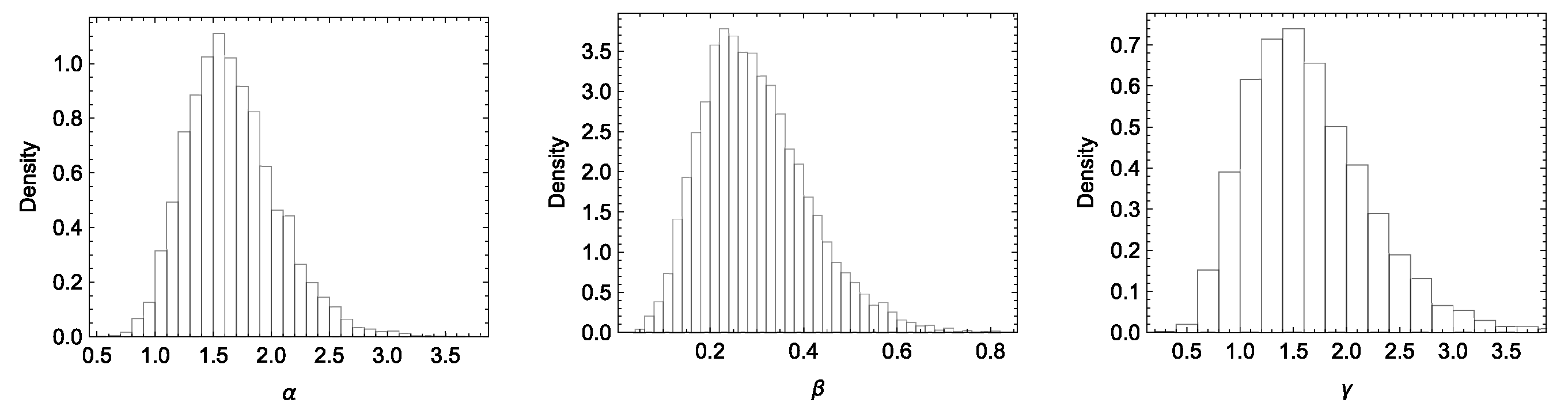
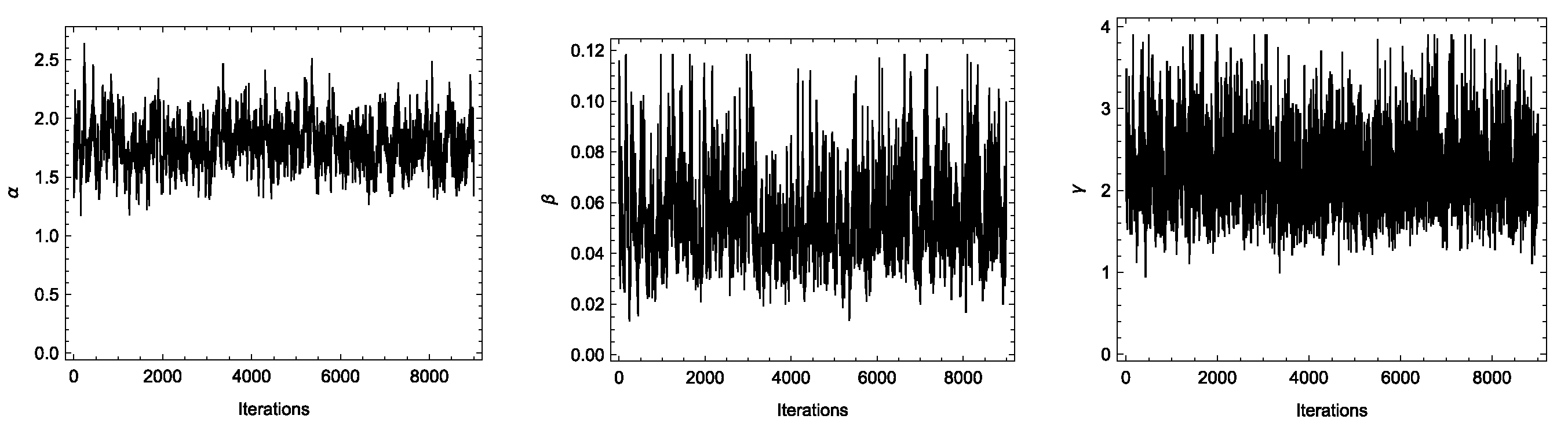
For the Bayesian estimation approach, informative priors are employed, where the hyperparameters are determined using the method of moments. This ensures that the Gamma prior distribution’s mean matches the corresponding parameter’s true value, with a prior variance set to 1. The MCMC procedure was run for 10,000 iterations, discarding the initial 1000 iterations as a burn-in period. In addition, a thinning process was applied, retaining every third observation to reduce autocorrelation.

The simulation results are presented in

Table 1. MSEs of the parameter estimates for Case 1.

			MLE	Bayesian (MCMC)			Bayesian (Lindley)
					LINEX			LINEX
$\mathbf{(}\mathit{n}\mathbf{,}\mathit{m}\mathbf{)}$	Scheme	Parameter		SE	$\mathit{c}\mathbf{=}\mathbf{1}$	$\mathit{c}\mathbf{=}\mathbf{-}\mathbf{1}$	SE	$\mathit{c}\mathbf{=}\mathbf{1}$	$\mathit{c}\mathbf{=}\mathbf{-}\mathbf{1}$
$(30,15)$	I	$\alpha$	0.0160	0.0367	0.0335	0.0403	0.0362	0.0493	0.0331
		$\beta$	0.0284	0.0291	0.0289	0.0298	0.0356	0.0343	0.0370
		$\gamma$	0.6331	0.3034	0.3872	0.4246	0.8944	0.7931	1.3292
	II	$\alpha$	0.0101	0.0305	0.0276	0.0339	0.0255	0.0253	0.0290
		$\beta$	0.0159	0.0214	0.0143	0.0233	0.0205	0.0196	0.0217
		$\gamma$	0.4224	0.3787	0.5468	0.3064	1.1201	0.7291	0.5339
	III	$\alpha$	0.0393	0.0762	0.0687	0.0846	0.0364	0.0350	0.0397
		$\beta$	0.0146	0.5921	0.5263	0.6710	0.0134	0.0132	0.0137
		$\gamma$	1.1186	0.3205	0.1746	1.0657	1.6375	1.1393	1.3124
$(50,30)$	I	$\alpha$	0.0063	0.0150	0.0140	0.0160	0.0101	0.0098	0.0105
		$\beta$	0.0164	0.0183	0.0179	0.0187	0.0165	0.0159	0.0171
		$\gamma$	0.4871	0.2740	0.3385	0.3628	0.8661	0.7730	1.1588
	II	$\alpha$	0.0093	0.0075	0.0070	0.0081	0.0067	0.0063	0.0074
		$\beta$	0.0099	0.0187	0.0113	0.0203	0.0118	0.0113	0.0123
		$\gamma$	0.5783	0.3591	0.5383	0.2752	0.9573	0.4941	0.6407
	III	$\alpha$	0.0335	0.0239	0.0231	0.0248	0.0303	0.0307	0.0302
		$\beta$	0.0094	0.2201	0.2099	0.2311	0.0091	0.0104	0.0111
		$\gamma$	0.6049	0.2531	0.1641	0.9402	0.9175	1.0911	1.0558
$(70,50)$	I	$\alpha$	0.0057	0.0070	0.0067	0.0074	0.0041	0.0040	0.0043
		$\beta$	0.0090	0.0099	0.0098	0.0100	0.0080	0.0078	0.0082
		$\gamma$	0.4166	0.1950	0.3818	0.3417	0.5465	0.6852	0.9053
	II	$\alpha$	0.0056	0.0050	0.0048	0.0051	0.0037	0.0035	0.0038
		$\beta$	0.0082	0.0152	0.0173	0.0162	0.0080	0.0080	0.0082
		$\gamma$	0.2618	0.2573	0.4765	0.2429	0.4960	0.3980	0.6557
	III	$\alpha$	0.0281	0.0016	0.0015	0.0016	0.0248	0.0249	0.0247
		$\beta$	0.0078	0.0061	0.0060	0.0063	0.0098	0.0094	0.0103
		$\gamma$	0.4046	0.0254	0.0187	0.0396	0.4440	0.7786	0.7924
$(100,70)$	I	$\alpha$	0.0040	0.0039	0.0038	0.3628	0.0023	0.0024	0.0023
		$\beta$	0.0068	0.0077	0.0076	0.8661	0.0060	0.0058	0.0062
		$\gamma$	0.2934	0.1620	0.3618	0.7730	0.3763	0.2113	0.6331
	II	$\alpha$	0.0045	0.0028	0.0027	0.0029	0.0025	0.0024	0.0025
		$\beta$	0.0057	0.0123	0.0200	0.0136	0.0051	0.0050	0.0052
		$\gamma$	0.2600	0.1459	0.4016	0.2173	0.3049	0.1266	0.5042
	III	$\alpha$	0.0220	0.0001	0.0001	0.0001	0.0129	0.0128	0.0131
		$\beta$	0.0061	0.0021	0.0020	0.0022	0.0109	0.0086	0.0096
		$\gamma$	0.2603	0.0099	0.0047	0.0190	0.4542	0.6947	0.7482

,

Table 2. ABs of the parameter estimates for Case 1.

			MLE	Bayesian (MCMC)			Bayesian (Lindley)
					LINEX			LINEX
$\mathbf{(}\mathit{n}\mathbf{,}\mathit{m}\mathbf{)}$	Scheme	Parameter		SE	$\mathit{c}\mathbf{=}\mathbf{1}$	$\mathit{c}\mathbf{=}\mathbf{-}\mathbf{1}$	SE	$\mathit{c}\mathbf{=}\mathbf{1}$	$\mathit{c}\mathbf{=}\mathbf{-}\mathbf{1}$
$(30,15)$	I	$\alpha$	0.0411	0.1112	0.1026	0.1201	0.0994	0.1031	0.0981
		$\beta$	−0.0085	−0.0474	−0.0606	−0.0333	0.0450	0.0335	0.0563
		$\gamma$	0.2679	−0.2347	−0.5543	0.2696	−0.1438	−0.8800	1.6569
	II	$\alpha$	0.0406	0.0818	0.0734	0.0906	0.0588	0.0564	0.0597
		$\beta$	0.0065	0.1017	0.0957	0.1079	0.0218	0.0150	0.0317
		$\gamma$	0.2112	−0.4623	−0.5846	0.2897	0.6689	−0.7895	0.6162
	III	$\alpha$	0.0576	0.1811	0.1677	0.1953	0.0808	0.0711	0.0915
		$\beta$	0.0451	0.5280	0.4913	0.5687	−0.0121	0.0547	0.0610
		$\gamma$	0.6091	0.3126	−0.0700	0.8900	0.2294	−0.6188	1.3202
$(50,30)$	I	$\alpha$	0.0305	0.0636	0.0594	0.0680	0.0385	0.0363	0.0404
		$\beta$	−0.0098	−0.0170	−0.0248	−0.0088	0.0222	0.0143	0.0298
		$\gamma$	0.2045	−0.1757	−0.4650	0.2900	−0.0651	−0.4476	1.0995
	II	$\alpha$	0.0275	0.0403	0.0365	0.0442	0.0277	0.0249	0.0298
		$\beta$	0.0075	0.0958	0.0916	0.1000	0.0213	0.0115	0.0275
		$\gamma$	0.1897	−0.3992	−0.6050	0.0809	0.2300	−0.4809	0.5248
	III	$\alpha$	0.0245	0.0232	0.0195	0.0270	0.0110	0.0076	0.0144
		$\beta$	0.0378	0.1190	0.1102	0.1282	0.0238	0.0514	0.0598
		$\gamma$	0.3985	0.3226	0.0528	0.7333	0.1576	−0.7676	1.1381
$(70,50)$	I	$\alpha$	0.0163	0.0478	0.0453	0.0503	0.0221	0.0202	0.0240
		$\beta$	0.0040	−0.0089	−0.0138	−0.0038	0.0126	−0.0012	0.0094
		$\gamma$	−0.0529	−0.2241	−0.4603	0.1213	0.1762	0.0664	0.6759
	II	$\alpha$	0.0195	0.0122	0.0098	0.0146	0.0168	0.0147	0.0190
		$\beta$	−0.0055	0.0476	0.0402	0.0553	−0.0057	0.0009	−0.0016
		$\gamma$	−0.0549	−0.3368	−0.6235	−0.0512	0.2268	−0.0164	0.5648
	III	$\alpha$	−0.1516	0.0055	0.0053	0.0057	−0.1278	−0.1281	−0.1273
		$\beta$	0.0230	−0.0011	−0.0013	−0.0009	0.0556	0.0176	0.0300
		$\gamma$	0.2384	0.0073	−0.0027	0.0202	−0.4156	−0.6277	0.8329
$(100,70)$	I	$\alpha$	0.0141	0.0279	0.0261	0.2900	0.0028	0.0016	0.0041
		$\beta$	0.0157	0.0014	−0.0024	−0.0651	0.0041	0.0047	0.0066
		$\gamma$	−0.0876	−0.1702	−0.3915	−0.4476	0.1127	−0.0379	0.4314
	II	$\alpha$	0.0117	0.0112	0.0095	0.0129	0.0072	0.0059	0.0086
		$\beta$	0.0053	0.0111	−0.0011	0.0241	0.0038	−0.0099	0.0028
		$\gamma$	−0.1090	−0.2541	−0.6498	−0.0852	0.0748	−0.0915	0.4406
	III	$\alpha$	−0.1781	0.0008	0.0007	0.0008	−0.1487	−0.1470	−0.1498
		$\beta$	−0.0252	0.0026	0.0045	0.0047	0.0577	−0.0214	−0.0029
		$\gamma$	−0.0496	0.0100	0.0069	0.0138	−1.1156	−0.3325	0.8074

,

Table 3. MSEs of the parameter estimates for Case 2.

			MLE	Bayesian (MCMC)			Bayesian (Lindley)
					LINEX			LINEX
$\mathbf{(}\mathit{n}\mathbf{,}\mathit{m}\mathbf{)}$	Scheme	Parameter		SE	$\mathit{c}\mathbf{=}\mathbf{1}$	$\mathit{c}\mathbf{=}\mathbf{-}\mathbf{1}$	SE	$\mathit{c}\mathbf{=}\mathbf{1}$	$\mathit{c}\mathbf{=}\mathbf{-}\mathbf{1}$
$(30,15)$	I	$\alpha$	0.2875	0.1789	0.1288	0.3213	0.1587	0.1516	0.2597
		$\beta$	0.2248	0.1678	0.1227	0.2655	0.1057	0.1300	0.1406
		$\gamma$	0.3051	0.1587	0.1064	0.4126	0.2201	0.1898	0.4843
	II	$\alpha$	0.3164	0.2590	0.1748	0.4480	0.1606	0.1199	0.4707
		$\beta$	0.2281	0.0935	0.0611	0.1749	0.1724	0.1154	0.1524
		$\gamma$	0.4440	0.1639	0.0957	0.4472	0.2618	0.1370	0.5173
	III	$\alpha$	0.5441	0.2795	0.1986	0.3448	0.1182	0.1183	0.3006
		$\beta$	0.1290	0.1728	0.2545	1.7084	0.0583	0.0580	0.0791
		$\gamma$	0.8333	1.2622	1.1395	1.9155	0.5922	0.1523	0.8335
$(50,30)$	I	$\alpha$	0.2808	0.1617	0.1274	0.2418	0.0917	0.0929	0.1413
		$\beta$	0.1438	0.0895	0.0792	0.1145	0.0458	0.0490	0.0664
		$\gamma$	0.2857	0.1609	0.0920	0.3038	0.0919	0.0665	0.2547
	II	$\alpha$	0.2575	0.1448	0.1167	0.2061	0.0807	0.0916	0.0870
		$\beta$	0.1512	0.0756	0.0600	0.1109	0.0616	0.0567	0.0914
		$\gamma$	0.1941	0.1302	0.0930	0.2356	0.1181	0.0783	0.2402
	III	$\alpha$	0.4440	0.2151	0.1517	0.3996	0.1160	0.1043	0.1568
		$\beta$	0.1639	0.0794	0.2239	1.6082	0.0557	0.0524	0.0720
		$\gamma$	0.0957	1.4753	0.6912	1.3913	0.1374	0.0880	0.3402
$(70,50)$	I	$\alpha$	0.2400	0.1637	0.1281	0.2298	0.0870	0.0830	0.1376
		$\beta$	0.1043	0.0729	0.0623	0.0914	0.0466	0.0468	0.0566
		$\gamma$	0.2931	0.1193	0.0880	0.2127	0.0982	0.0620	0.2172
	II	$\alpha$	0.1987	0.1450	0.1226	0.1898	0.0664	0.0788	0.1029
		$\beta$	0.1163	0.0761	0.0572	0.0992	0.0549	0.0484	0.0739
		$\gamma$	0.1217	0.0848	0.0673	0.1242	0.0981	0.0773	0.1410
	III	$\alpha$	0.2857	0.2106	0.1445	0.2952	0.0892	0.0952	0.1574
		$\beta$	0.1609	0.0831	0.1180	0.9053	0.0429	0.0442	0.0498
		$\gamma$	0.0920	0.7612	0.6368	0.7127	0.1226	0.0859	0.1869
$(100,70)$	I	$\alpha$	0.1885	0.0994	0.0877	0.1252	0.0592	0.0767	0.1335
		$\beta$	0.0716	0.0593	0.0524	0.0703	0.0420	0.0385	0.0526
		$\gamma$	0.1389	0.1122	0.0852	0.1765	0.0832	0.0385	0.1320
	II	$\alpha$	0.1469	0.1022	0.0913	0.1225	0.0624	0.0770	0.1027
		$\beta$	0.0815	0.0652	0.0530	0.0817	0.0506	0.0468	0.0601
		$\gamma$	0.1267	0.0846	0.0719	0.1088	0.0706	0.0415	0.1275
	III	$\alpha$	0.1429	0.1664	0.1302	0.2147	0.0887	0.0757	0.1200
		$\beta$	0.0486	0.0734	0.0603	0.9684	0.0380	0.0321	0.0436
		$\gamma$	0.0990	0.8187	0.5502	0.5856	0.0742	0.0540	0.1099

,

Table 4. ABs of the parameter estimates for Case 2.

			MLE	Bayesian (MCMC)			Bayesian (Lindley)
					LINEX			LINEX
$\mathbf{(}\mathit{n}\mathbf{,}\mathit{m}\mathbf{)}$	Scheme	Parameter		SE	$\mathit{c}\mathbf{=}\mathbf{1}$	$\mathit{c}\mathbf{=}\mathbf{-}\mathbf{1}$	SE	$\mathit{c}\mathbf{=}\mathbf{1}$	$\mathit{c}\mathbf{=}\mathbf{-}\mathbf{1}$
$(30,15)$	I	$\alpha$	0.1039	0.1261	−0.0322	0.3203	0.0571	−0.1179	0.2379
		$\beta$	0.0489	0.1458	0.0321	0.2902	0.0467	−0.0494	0.1890
		$\gamma$	0.2146	0.1540	0.0536	0.3855	0.2673	0.1245	0.5589
	II	$\alpha$	0.1794	0.1792	0.0183	0.3718	0.0351	−0.0853	0.1334
		$\beta$	0.0950	0.1297	0.0951	0.2636	0.0539	−0.0671	0.1299
		$\gamma$	0.2513	0.1615	0.0191	0.4072	0.3023	0.1669	0.5800
	III	$\alpha$	0.2629	0.3321	0.2291	0.3779	0.1316	−0.0732	0.3491
		$\beta$	−0.0183	0.6112	0.7739	1.9650	−0.0143	−0.0865	0.1068
		$\gamma$	0.5641	1.2297	0.9446	1.8337	0.0872	0.0726	0.6547
$(50,30)$	I	$\alpha$	0.0907	0.1250	−0.0314	0.2191	0.0521	−0.0730	0.2083
		$\beta$	0.0444	0.0571	−0.0288	0.1142	−0.0179	−0.0945	0.0777
		$\gamma$	0.1837	0.1501	0.0183	0.2928	0.2192	0.1049	0.3852
	II	$\alpha$	0.1250	0.0861	−0.0211	0.2054	−0.0323	−0.1372	0.0993
		$\beta$	0.0900	0.1283	0.0520	0.1695	0.0424	−0.0271	0.1296
		$\gamma$	0.1063	0.0884	−0.0046	0.2283	0.2095	0.0955	0.3302
	III	$\alpha$	0.2513	0.2905	0.2058	0.4468	0.0376	−0.0730	0.1675
		$\beta$	0.1615	0.4613	0.6877	1.6658	0.0453	−0.0344	0.0804
		$\gamma$	0.0191	0.9942	0.7140	1.6518	0.1835	0.0603	0.3628
$(70,50)$	I	$\alpha$	0.0592	0.0838	0.0304	0.2319	0.0291	−0.0709	0.1524
		$\beta$	−0.0057	0.0657	0.0157	0.1220	−0.0098	−0.0603	0.0706
		$\gamma$	0.1816	0.0887	0.0157	0.1894	0.1822	0.1069	0.2924
	II	$\alpha$	0.0639	0.0611	−0.0224	0.1538	0.0564	−0.0329	0.1613
		$\beta$	0.0870	0.0976	0.0266	0.1672	0.0178	0.0050	0.1096
		$\gamma$	0.0728	0.0537	−0.0078	0.1336	0.1114	0.0708	0.1868
	III	$\alpha$	0.1837	0.2320	0.1704	0.3841	0.0185	−0.0283	0.1311
		$\beta$	0.1501	0.4673	0.3507	0.8591	0.0089	−0.0090	0.0596
		$\gamma$	0.0183	0.8144	0.6722	0.9653	0.1524	0.0329	0.2344
$(100,70)$	I	$\alpha$	0.0482	0.0433	−0.0259	0.1193	0.0179	−0.0238	0.1309
		$\beta$	−0.0084	0.0607	0.0237	0.1008	0.0304	−0.0130	0.0464
		$\gamma$	0.0496	0.0644	0.0112	0.1387	0.1129	0.0546	0.1757
	II	$\alpha$	0.0632	0.0479	−0.0120	0.1121	0.0278	−0.0412	0.1064
		$\beta$	0.0333	0.0924	0.0232	0.1489	0.0131	−0.0018	0.0568
		$\gamma$	0.0329	0.0238	−0.0215	0.0790	0.1283	0.0348	0.1879
	III	$\alpha$	0.0659	0.2233	0.0867	0.2979	0.0486	0.0053	0.1252
		$\beta$	0.0278	0.3712	0.2971	0.9076	0.0275	−0.0065	0.0573
		$\gamma$	0.0535	0.7960	0.5576	0.9404	0.0947	0.0018	0.1535

,

Table 5. MSEs of the parameter estimates for Case 3.

			MLE	Bayesian (MCMC)			Bayesian (Lindley)
					LINEX			LINEX
$\mathbf{(}\mathit{n}\mathbf{,}\mathit{m}\mathbf{)}$	Scheme	Parameter		SE	$\mathit{c}\mathbf{=}\mathbf{1}$	$\mathit{c}\mathbf{=}\mathbf{-}\mathbf{1}$	SE	$\mathit{c}\mathbf{=}\mathbf{1}$	$\mathit{c}\mathbf{=}\mathbf{-}\mathbf{1}$
$(30,15)$	I	$\alpha$	0.0562	0.0513	0.0427	0.0629	0.0463	0.0585	0.0490
		$\beta$	0.0636	0.0541	0.0492	0.0611	0.0498	0.0447	0.0573
		$\gamma$	0.7434	0.2402	0.1569	0.7764	0.5704	0.2353	0.7476
	II	$\alpha$	0.0620	0.0476	0.0400	0.0574	0.0485	0.1378	0.0489
		$\beta$	0.0624	0.0465	0.0421	0.0524	0.0513	0.0468	0.0575
		$\gamma$	0.7033	0.1844	0.1700	0.6304	0.9216	0.3095	0.9741
	III	$\alpha$	0.0842	0.0959	0.0795	0.1167	0.0820	0.0687	0.0987
		$\beta$	0.0484	0.6744	0.6287	0.7247	0.0389	0.0427	0.0929
		$\gamma$	0.7915	0.9203	0.5482	1.4401	0.8347	0.8530	0.9273
$(50,30)$	I	$\alpha$	0.0363	0.0248	0.0220	0.0283	0.0223	0.0203	0.0255
		$\beta$	0.0296	0.0232	0.0223	0.0246	0.0245	0.0233	0.0263
		$\gamma$	0.7016	0.2601	0.1714	0.6055	0.2498	0.1652	0.4427
	II	$\alpha$	0.0307	0.0181	0.0163	0.0204	0.0205	0.0187	0.0232
		$\beta$	0.0223	0.0230	0.0216	0.0247	0.0187	0.0181	0.0197
		$\gamma$	0.6857	0.2463	0.1566	0.6156	0.1993	0.1074	0.6358
	III	$\alpha$	0.0315	0.0806	0.0741	0.0878	0.0587	0.0596	0.0577
		$\beta$	0.0133	0.3730	0.3201	0.4365	0.0255	0.0212	0.0356
		$\gamma$	0.6683	0.5411	0.4994	0.8407	0.5004	0.4618	0.6956
$(70,50)$	I	$\alpha$	0.0188	0.0177	0.0162	0.0194	0.0133	0.0122	0.0146
		$\beta$	0.0216	0.0150	0.0147	0.0154	0.0189	0.0186	0.0195
		$\gamma$	0.5356	0.2202	0.1542	0.4434	0.2196	0.1617	0.4438
	II	$\alpha$	0.0184	0.0159	0.0147	0.0172	0.0128	0.0120	0.0140
		$\beta$	0.0143	0.0117	0.0114	0.0121	0.0130	0.0128	0.0133
		$\gamma$	0.4288	0.2307	0.1528	0.5008	0.1603	0.1053	0.4869
	III	$\alpha$	0.0408	0.0197	0.0199	0.0195	0.0460	0.0484	0.0451
		$\beta$	0.0160	0.2128	0.2104	0.2154	0.0187	0.0184	0.0189
		$\gamma$	0.5718	0.3269	0.2110	0.6531	0.3899	0.3362	0.6936
$(100,70)$	I	$\alpha$	0.0137	0.0100	0.0095	0.0107	0.0108	0.0102	0.0115
		$\beta$	0.0135	0.0112	0.0109	0.0115	0.0122	0.0121	0.0123
		$\gamma$	0.3989	0.2160	0.1551	0.3960	0.1995	0.1470	0.3064
	II	$\alpha$	0.0115	0.0104	0.0098	0.0112	0.0085	0.0081	0.0090
		$\beta$	0.0107	0.0106	0.0104	0.0109	0.0100	0.0098	0.0103
		$\gamma$	0.3825	0.1717	0.1357	0.3070	0.1719	0.0508	0.4221
	III	$\alpha$	0.0499	0.0045	0.0043	0.0047	0.0305	0.0289	0.0326
		$\beta$	0.0161	0.0607	0.0590	0.0625	0.0146	0.0148	0.0141
		$\gamma$	0.5653	0.3163	0.1483	0.5234	0.3855	0.1392	0.5600

,

Table 6. ABs of the parameter estimates for Case 3.

			MLE	Bayesian (MCMC)			Bayesian (Lindley)
					LINEX			LINEX
$\mathbf{(}\mathit{n}\mathbf{,}\mathit{m}\mathbf{)}$	Scheme	Parameter		SE	$\mathit{c}\mathbf{=}\mathbf{1}$	$\mathit{c}\mathbf{=}\mathbf{-}\mathbf{1}$	SE	$\mathit{c}\mathbf{=}\mathbf{1}$	$\mathit{c}\mathbf{=}\mathbf{-}\mathbf{1}$
$(30,15)$	I	$\alpha$	0.0784	0.0957	0.0740	0.1198	0.0895	0.0807	0.1071
		$\beta$	0.0403	0.0279	0.0021	0.0558	0.0464	0.0197	0.0741
		$\gamma$	0.2638	0.1219	−0.1189	0.5556	0.2468	−0.1073	0.6934
	II	$\alpha$	0.1108	0.1036	0.0826	0.1263	0.1012	0.1060	0.1167
		$\beta$	0.0587	0.0309	0.0096	0.0536	0.0548	0.0338	0.0775
		$\gamma$	0.2200	0.1155	−0.1841	0.4803	0.2265	−0.0640	0.6496
	III	$\alpha$	0.1096	0.1956	0.1672	0.2267	0.1318	0.1044	0.1601
		$\beta$	−0.1865	0.5218	0.4963	0.5487	−0.1686	−0.1810	−0.1565
		$\gamma$	0.3819	0.6724	0.3188	0.8107	−0.1558	−0.2949	0.7141
$(50,30)$	I	$\alpha$	0.0370	0.0554	0.0431	0.0685	0.0463	0.0349	0.0587
		$\beta$	0.0073	0.0066	−0.0072	0.0211	0.0174	0.0028	0.0319
		$\gamma$	0.2476	0.1404	−0.0482	0.4513	0.2332	−0.0905	0.5410
	II	$\alpha$	0.0519	0.0434	0.0326	0.0548	0.0547	0.0438	0.0665
		$\beta$	−0.0045	0.0215	0.0100	0.0335	0.0012	−0.0103	0.0127
		$\gamma$	0.1758	0.0961	−0.1004	0.4323	0.2181	−0.0602	0.5269
	III	$\alpha$	0.0105	0.1672	0.1537	0.1812	0.0242	−0.1609	0.0355
		$\beta$	−0.0404	0.4026	0.3645	0.4440	−0.0379	−0.0467	−0.0287
		$\gamma$	0.3647	0.3244	−0.3476	0.7892	0.1178	−0.0697	0.5576
$(70,50)$	I	$\alpha$	0.0184	0.0462	0.0379	0.0548	0.0246	0.0160	0.0333
		$\beta$	−0.0072	−0.0013	−0.0099	0.0076	−0.0020	−0.0111	0.0071
		$\gamma$	0.2137	0.0967	−0.0493	0.3232	0.1051	0.0561	0.5328
	II	$\alpha$	0.0222	0.0397	0.0322	0.0474	0.0194	0.0112	0.0278
		$\beta$	−0.0056	0.0066	−0.0007	0.0142	−0.0042	−0.0118	0.0034
		$\gamma$	0.1703	0.0513	−0.0357	0.3551	0.0911	0.0420	0.4715
	III	$\alpha$	−0.0837	−0.0412	−0.0455	−0.0366	−0.0968	−0.1036	−0.0915
		$\beta$	0.0096	−0.0449	−0.2131	−0.2084	−0.0085	−0.0132	−0.0161
		$\gamma$	−0.0533	−0.2938	−0.0638	−0.2163	0.0578	−0.0515	0.2842
$(100,70)$	I	$\alpha$	0.0129	0.0237	0.0179	0.0297	0.0168	0.0105	0.0232
		$\beta$	−0.0138	0.0043	−0.0021	0.0109	−0.0111	−0.0178	−0.0046
		$\gamma$	0.1773	0.0963	−0.0243	0.2736	−0.0608	−0.0127	0.4447
	II	$\alpha$	0.0114	0.0363	0.0308	0.0420	0.0092	0.0034	0.0150
		$\beta$	0.0044	0.0047	−0.0006	0.0101	0.0047	−0.0008	0.0103
		$\gamma$	0.1542	0.0380	−0.0778	0.2091	−0.0633	0.0753	0.4155
	III	$\alpha$	−0.1425	0.0148	0.0140	0.0156	−0.1603	0.0130	−0.1566
		$\beta$	0.0163	−0.0108	0.0436	0.0462	0.0012	−0.0037	0.0066
		$\gamma$	−0.1362	0.1342	0.0983	0.1869	0.0507	−0.0231	0.2267

and

Table 7. AW and CP for $95\%$ confidence intervals for the parameters for all cases.

			Case 1				Case 2				Case 3
			ACIs		CRIs		ACIs		CRIs		ACIs		CRIs
$\mathbf{(}\mathit{n}\mathbf{,}\mathit{m})$	Scheme	Parameter	AW	CP	AW	CP	AW	CP	AW	CP	AW	CP	AW	CP
$(30,15)$	I	$\alpha$	0.5693	0.993	0.4966	0.847	3.3376	0.980	2.2633	1.000	0.9560	0.980	0.8042	0.975
		$\beta$	0.7385	0.967	0.6176	0.913	2.6085	0.980	1.9257	0.990	0.9918	0.953	0.8871	0.945
		$\gamma$	8.5658	0.993	3.3624	1.000	3.4398	0.993	2.2074	1.000	5.2025	0.933	2.9988	1.000
	II	$\alpha$	0.5934	0.993	0.4909	0.913	3.3221	1.000	2.2588	0.990	0.9420	0.980	0.7885	0.975
		$\beta$	0.6185	0.960	0.6032	0.973	2.6103	0.980	1.8593	1.000	0.9171	0.953	0.7978	0.915
		$\gamma$	7.1194	0.987	3.4445	1.000	3.4665	0.993	2.2626	1.000	5.3690	0.953	2.9623	0.995
	III	$\alpha$	0.6654	0.980	0.6252	0.850	3.1977	0.967	2.0803	0.980	1.0005	0.973	0.9232	0.915
		$\beta$	0.5530	0.920	0.9762	0.940	1.9410	0.980	2.9546	0.270	0.7322	0.880	1.0306	0.860
		$\gamma$	8.0606	1.000	3.7211	1.000	4.7663	0.993	4.0696	0.900	5.9433	0.973	3.9266	0.995
$(50,30)$	I	$\alpha$	0.3912	0.980	0.3475	0.900	2.5650	0.993	1.9099	0.980	0.6737	0.967	0.6069	0.945
		$\beta$	0.5472	0.913	0.4861	0.893	1.8235	0.967	1.4540	0.980	0.6953	0.940	0.6534	0.965
		$\gamma$	7.8141	0.973	3.2092	0.987	2.4471	0.993	1.7830	0.980	3.8564	0.940	2.5793	0.985
	II	$\alpha$	0.3873	0.987	0.3324	0.967	2.3533	0.987	1.8298	0.960	0.6713	0.973	0.5687	0.975
		$\beta$	0.4574	0.980	0.4684	0.980	1.7904	0.987	1.4421	1.000	0.6169	0.960	0.5942	0.965
		$\gamma$	5.7745	0.993	3.0769	0.993	2.2482	0.980	1.7590	0.980	3.9594	0.947	2.6664	0.995
	III	$\alpha$	0.4539	0.880	0.2923	0.900	2.2441	0.973	1.7943	0.940	0.6356	0.947	0.6289	0.940
		$\beta$	0.4480	0.987	0.3810	0.860	1.4920	0.987	2.2883	0.860	0.5506	0.960	0.8087	0.915
		$\gamma$	4.1496	0.953	2.7910	1.000	2.4092	0.973	3.1103	0.890	4.2813	0.940	3.5018	0.885
$(70,50)$	I	$\alpha$	0.3202	0.993	0.2708	0.887	2.0243	0.940	1.7232	0.980	0.5407	0.940	0.4998	0.955
		$\beta$	0.4303	0.980	0.3829	0.960	1.3928	0.927	1.2530	0.980	0.5391	0.933	0.5140	0.960
		$\gamma$	3.4169	0.940	2.8451	0.987	1.9226	0.980	1.4872	0.970	3.1074	0.940	2.2340	0.985
	II	$\alpha$	0.3156	1.000	0.2649	0.947	1.9064	0.980	1.6161	0.990	0.5248	0.967	0.4740	0.965
		$\beta$	0.3686	0.940	0.4276	0.887	1.3514	0.947	1.1970	0.970	0.4897	0.940	0.4757	0.970
		$\gamma$	3.2269	0.967	2.7834	0.967	1.5815	0.967	1.3997	0.980	2.9917	0.967	2.2692	0.995
	III	$\alpha$	0.2503	0.973	0.0152	0.980	1.9018	0.927	1.6250	0.960	0.5066	0.820	0.2839	0.875
		$\beta$	0.3917	0.987	0.0120	0.970	1.2408	0.980	1.6004	0.860	0.4935	0.947	0.1574	0.885
		$\gamma$	4.6328	0.973	0.1170	1.000	1.6821	0.953	2.0296	0.920	2.9139	0.840	0.9031	0.960
$(100,70)$	I	$\alpha$	0.2639	0.973	0.2285	0.927	1.7485	0.947	1.4730	0.960	0.4543	0.940	0.4185	0.965
		$\beta$	0.3689	0.993	0.3364	0.927	1.2230	0.960	1.0742	0.970	0.4549	0.933	0.4454	0.960
		$\gamma$	2.5782	0.920	2.7563	0.960	1.4423	0.960	1.2827	0.940	2.5646	0.960	1.9976	0.975
	II	$\alpha$	0.2643	0.973	0.2266	0.947	1.5924	0.980	1.3652	0.980	0.4370	0.960	0.4074	0.970
		$\beta$	0.3131	0.967	0.3537	0.853	1.1012	0.940	1.0368	0.970	0.4166	0.947	0.4021	0.945
		$\gamma$	2.4278	0.927	2.5392	0.953	1.4029	0.953	1.1872	0.970	2.5503	0.980	1.9687	0.960
	III	$\alpha$	0.1997	0.940	0.0027	1.000	1.5757	0.967	1.3805	0.950	0.4205	0.827	0.0583	0.965
		$\beta$	0.3502	0.973	0.0052	0.990	1.0231	0.987	1.4101	0.870	0.4208	0.920	0.0672	0.860
		$\gamma$	3.8110	0.980	0.0339	1.000	1.3555	0.973	1.8112	0.870	2.6928	0.913	0.3896	0.910

. Various conclusions about the performance of estimators are drawn as follows:

• All estimation methods exhibit satisfactory behavior in terms of the MSEs and AB presented in Table 1, Table 2, Table 3, Table 4, Table 5 and Table 6, indicating their validity across different schemes and sample sizes.
• As the sample size increases, the MSEs and ABs across all estimation methods and parameters tend to decrease.
• Censoring Scheme I generally shows lower MSEs for most parameter estimates compared to Schemes II and III. This trend implies that Scheme I might be more favorable for achieving accurate estimates.
• Across all estimation methods, parameter $\gamma$ tends to exhibit larger MSE and AB values compared to parameters $\alpha$ and $\beta$.
• For Bayesian estimates obtained through Lindley’s approximation or MCMC techniques, the choice of loss function affects MSE and AB. Symmetric loss functions (the SE loss) consistently produce preferable results compared to asymmetric loss functions.
• The MLE and MCMC with SE loss offer the most balanced performance in terms of AB and MSE across all cases, with MCMC slightly outperforming in larger samples. Lindley’s method, while effective for $\alpha$ and $\beta$, appears less reliable for $\gamma$.
• Censoring Scheme III, which tends to remove units later in the test, consistently shows higher MSEs and AB across all parameters and estimation methods, particularly in smaller samples. In contrast, Schemes I and II provide more reliable performance with generally lower MSEs and AB, supporting more accurate estimation.
• According to the results of the interval estimates shown in Table 7, the AWs for ACIs and CRIs become narrower as the sample size increases and the CPs are mostly close to the nominal level. The CRIs are narrower and provide better coverage probabilities.
• The average values of the optimal stress change time $\tau$ based on the A-optimality (AO) and D-optimality (DO) are listed in

  Table 8. The average optimal transition stress changing time $\tau$ using D-optimality and A-optimality.

  		Case 1		Case 2		Case 3
  $\mathbf{(}\mathit{n}\mathbf{,}\mathit{m}\mathbf{)}$	Scheme	${\mathsf{\tau }}_{\mathit{D}}^{\mathbf{*}}$	${\mathsf{\tau }}_{\mathit{A}}^{\mathbf{*}}$	${\mathsf{\tau }}_{\mathit{D}}^{\mathbf{*}}$	${\mathsf{\tau }}_{\mathit{A}}^{\mathbf{*}}$	${\mathsf{\tau }}_{\mathit{D}}^{\mathbf{*}}$	${\mathsf{\tau }}_{\mathit{A}}^{\mathbf{*}}$
  $(30,15)$	I	2.4662	2.5026	1.2736	1.1610	2.3448	2.3637
  	II	2.6504	2.7422	1.3027	1.1694	2.2563	2.3580
  	III	2.3457	2.3489	1.5672	1.0954	2.0579	1.9237
  $(50,30)$	I	2.5080	2.5625	1.2219	1.1492	2.3451	2.3570
  	II	2.4122	2.5088	1.4892	1.2116	2.4969	2.5634
  	III	2.2568	2.2976	1.5582	0.9120	2.0468	2.0634
  $(70,50)$	I	2.2456	2.4714	1.4853	1.2083	2.4032	2.4063
  	II	2.4104	2.4598	1.3739	1.1401	2.5099	2.5477
  	III	2.1158	2.1558	1.2341	1.0878	1.9472	1.9290
  $(100,70)$	I	2.4472	2.4869	1.3896	1.1872	2.4918	2.4932
  	II	2.4010	2.4450	1.5321	1.2777	2.3262	2.3555
  	III	1.9895	2.0936	1.0197	1.1091	2.1087	2.0600

  . The values of $\tau$ for both the AO and the DO methods are relatively close within each scheme.
• The MLE demonstrates competitive performance across all cases, particularly for smaller sample sizes. Its simplicity and computational efficiency make it a practical choice for applications where quick and reliable estimates are needed.
• The MCMC Bayesian estimates with SE loss show slightly better performance in larger samples, where the MLE remains robust and consistent, especially for parameters $\alpha$ and $\beta$.

7. Application to Real Data

This section explores three examples based on real-world data: two from engineering and one from medicine. The engineering cases focus on analyzing failure times under both normal and accelerated stress conditions, illustrating how to determine the optimal stress change time, $\tau$, to reduce testing duration while ensuring accurate reliability assessments. Additionally, they demonstrate the use of maintenance optimization in repairable systems. In contrast, the medical example applies the methods to study disease progression, incorporating censored data to enhance treatment strategies and improve patient outcomes.

7.1. Light Bulb Data

The dataset utilized in this analysis originates from an SSPALT experiment conducted by [31]. In this experiment, a total of 64 light bulbs were subjected to a life test at an initial stress level of $2.25\mathrm{V}$, representing normal operating conditions. At a predetermined time of $\tau =96$ h, the stress level increased to an accelerated condition of $2.44\mathrm{V}$. During the experiment, $n=53$ failures were recorded out of the 64 tested samples. These failure times are presented in

Table 9. Failure times observed under normal operating conditions ($2.25\mathrm{V}$) and accelerated stress conditions ($2.44\mathrm{V}$), with a stress change point at $\tau =96$ h.

Normal stress (before $\tau =96.0$)	12.07, 14.0, 17.95, 19.5, 22.1, 23.11, 24.0, 24.0, 25.1, 26.46, 26.58, 26.9,
	28.06, 34.0, 36.13, 36.64, 40.85, 41.11, 42.63, 44.1, 46.3, 52.51, 54.0, 58.09,
	62.68, 64.17, 72.25, 73.13, 83.63, 86.9, 90.09, 91.22, 91.56, 94.38
Accelerated stress (after $\tau =96.0$)	97.71, 101.53, 102.1, 105.1, 105.11, 109.2, 112.11, 114.4, 117.9, 119.58,
	120.2, 121.9, 122.5, 123.6, 126.5, 126.95, 129.25, 130.1, 136.31

.

To validate the PHL distribution as a suitable model for the complete set of data, we performed a goodness-of-fit analysis. This step establishes the PHL distribution as the baseline model before applying a more advanced modeling.

Table 10. The MLE, confidence interval, KS statistic, and the p-value for light bulb data.

Parameter	MLE	95% ACIs	KS	p-Value
$\alpha$	1.6297	(1.2397, 2.0197)	0.1207	0.4227
$\beta$	0.0011	(0.00, 0.0031)

presents the fitting results including MLEs for the parameter, Kolmogorov–Smirnov (KS), and its p-value. The p-value exceeded $0.05$, which suggests that it was well modeled by the PHL distribution. This result is further supported by Figure 4, which displays the estimated pdf with the observed histogram of the data, the estimated survival function compared with the Kaplan–Meier curve, and QQ-plots to assess the distributional fit.

To generate the ATIIPC sample, we consider $n=53$, $m=30$, $\tau =96$, and a predetermined experiment duration of $T=115$. The censoring scheme $R=(0^{*14},3,2^{*5},1^{*10})$, where $a^{*k}$ means that a is repeated k consecutively, was employed. The generated ATIIPC sample for the SSPALT experiment is presented in

Table 11. The generated ATIIPC sample from light bulb data.

Normal stress (before $\tau =96.0$)	12.07, 14., 17.95, 19.5, 22.1, 23.11, 24., 24., 25.1, 26.46, 34., 40.85,
	83.63, 90.09, 91.56
Accelerated stress (after $\tau =96.0$)	97.71, 101.53, 102.1, 105.1, 105.11, 109.2, 112.11, 114.4, 117.9, 119.58,
	97.71, 102.1, 105.11, 112.11, 117.9, 120.2, 121.9, 122.5, 123.6, 126.5, 126.95, 129.25

. Since the ATIIPC process permits modifications to the censoring scheme during the experiment, the observations extended beyond the predetermined duration of $T=115$. Consequently, the censoring scheme was adjusted to $R=(0^{*14},3,2^{*5},1^{*6},0^{*3},4)$ to account for the extended experimental period.

In

Table 12. Point, interval estimates for the parameters, and optimal values of $\tau$ for light bulb data.

		Lindley			MCMC					Optimal Stress Changing Time
			LINEX			LINEX
Parameter	MLE	SE	$\mathit{c}\mathbf{=}\mathbf{1}$	$\mathit{c}\mathbf{=}\mathbf{-}\mathbf{1}$	SE	$\mathit{c}\mathbf{=}\mathbf{1}$	$\mathit{c}\mathbf{=}\mathbf{-}\mathbf{1}$	ACIs	CrIs	${\mathsf{\tau }}_{\mathit{D}}^{\mathbf{*}}$	${\mathsf{\tau }}_{\mathit{A}}^{\mathbf{*}}$
$\alpha$	1.0850	1.0775	1.0562	1.0992	1.4041	1.3787	1.4308	(0.6765, 1.4935)	(0.9995, 1.8543)	85.688	79.303
$\beta$	0.0070	0.0102	0.0102	0.0103	0.00254	0.00254	0.00255	(0.00, 0.0200)	(0.0002, 0.0104)
$\gamma$	2.8392	3.1473	2.4107	3.6052	2.5216	2.3701	2.7052	(0.2942, 5.3841)	(1.5260, 3.7573)

the MLEs, Bayesian estimates, the corresponding $95\%$ confidence intervals, and the optimal values of $\tau$ under the two optimality criteria ${\tau }_D^{*}$ and ${\tau }_A^{*}$ are provided. Bayesian estimates were obtained using informative gamma priors for the parameters, where the hyperparameters were estimated to give a prior mean equal to the MLEs and a variance of $0.5$. The MCMC algorithm was executed for 100,000 iterations, discarding the first 10,000 iterations as burn-in. Every 10th iteration was retained to reduce autocorrelation, yielding 9000 sampled values for each MCMC chain. To assess the convergence of the MCMC chains, histograms of the sampled values for each parameter are presented in Figure 5, while the corresponding trace plots are shown in Figure 6. These figures demonstrate that the MCMC chains for the parameters exhibit good mixing and converge effectively to their respective posterior distributions. By analyzing failure times under normal and accelerated stress conditions, we demonstrate how the optimal stress change time $\tau$ can be determined to minimize testing duration while maintaining accurate reliability predictions. By optimizing $\tau$, manufacturers can design accelerated life tests that provide reliable results in a shorter time frame, enabling faster product development and quality assurance. This is especially critical in industries such as electronics, where rapid innovation and competitive market pressures demand quick yet accurate reliability assessments.

7.2. Time-Between-Failures Data

The dataset represents the time between failures in a repairable system obtained from [32]. First, we assessed the adequacy of the PHL distribution for the data by estimating the parameters using MLEs and then evaluating the KS test statistic and its corresponding p-value. The goodness-of-fit results are presented in

Table 13. The MLE, confidence interval, KS statistic, and p-value for time-between-failures data.

Parameter	MLE	95% ACIs	KS	p-Value
$\alpha$	1.2368	(0.8836, 1.5900)	0.0793	0.9917
$\beta$	0.7623	(0.4350, 1.0896)

. We concluded that the PHL distribution provides an excellent fit to the data. In addition, we visually assessed the goodness-of-fit by plotting a histogram of the data alongside the fitted density function. Furthermore, we compared the Kaplan–Meier curve with the estimated survival curve and generated a QQ-plot of the PHL distribution (see Figure 7).

To generate the ATIIPC scheme under SSPALT, we set $\tau =1.2$, $\gamma =1.8$, $n=30$, and $m=15$, with a censoring scheme $R=(3^{*2},2,0^{*3},1^{*7},0^{*2})$. The generated data are presented in

Table 14. The generated ATIIPC scheme from time-between-failures data.

Normal Condition: (Before $\tau =1.2$)	0.11, 0.59, 0.74, 1.06, 1.17
Stress Condition: (After $\tau =1.2$)	1.23, 1.23, 1.43, 1.49, 1.82, 1.86, 1.97, 2.23, 2.37, 2.46

. Observations extended beyond the predetermined duration of $T=1.8$, prompting an adjustment to the censoring scheme as $R=(3^{*2},2,0^{*3},1^{*4},0^{*4},3)$. Under these conditions, MLEs, Bayesian estimates, and confidence intervals $95\%$ are shown in

Table 15. Point, interval estimates for the parameters, and optimal values of $\tau$ for time-between-failures data.

		Lindley			MCMC					Optimal Stress Changing Time
			LINEX			LINEX
Parameter	MLE	SE	$\mathit{c}\mathbf{=}\mathbf{1}$	$\mathit{c}\mathbf{=}\mathbf{-}\mathbf{1}$	SE	$\mathit{c}\mathbf{=}\mathbf{1}$	$\mathit{c}\mathbf{=}\mathbf{-}\mathbf{1}$	ACIs	CrIs	${\mathsf{\tau }}_{\mathit{D}}^{\mathbf{*}}$	${\mathsf{\tau }}_{\mathit{A}}^{\mathbf{*}}$
$\alpha$	1.4792	1.4098	1.2570	1.5835	1.6617	1.5900	1.7468	(0.3053, 2.6531)	(1.0181, 2.5446)	1.1160	1.1161
$\beta$	0.3273	0.3241	0.3155	0.3328	0.2960	0.2898	0.3026	(0.0687, 0.5858)	(0.1174, 0.5591)
$\gamma$	1.6954	2.7509	1.8087	2.7953	1.6440	1.4995	1.8483	(0.00, 4.3947)	(0.7562, 3.0132)

. Histograms and trace plots (Figure 8 and Figure 9) confirm that the MCMC chains for $\alpha$, $\beta$, and $\gamma$ mix well and converge effectively to their posterior distributions. This analysis highlighted the utility of the methods in maintenance optimization for repairable systems. By modeling the time between failures, the results can inform maintenance schedules, reducing downtime and improving operational efficiency in industries such as manufacturing and transportation.

7.3. HIV Infection to AIDS

This section examines a real-world dataset that tracks the progression of HIV infection to AIDS among men over nearly 15 years. The data, derived from the US Centers for Disease Control and Prevention (CDC), highlight that by 1996, $54\%$ of diagnosed adult AIDS cases in the United States were attributed to close contact with HIV-positive individuals. Furthermore, $40\%$ of the new AIDS cases reported in that same year were related to similar exposures. Among the $54\%$, people who also used injection drugs accounted for $7\%$ of the cumulative cases and $5\%$ of new cases.

This dataset, collected during the advent of combination antiretroviral therapy in 1996, has been frequently cited in studies, including those by [33,34], and for its value in understanding disease progression. Some observations involve patients whose results were censored or who did not develop AIDS during the study period. In this analysis, we implemented the SSPALT model by focusing on the predetermined number of failures observed, i.e., 150, out of a complete dataset comprising 222 individuals. These observations were extracted from [7].

To validate the PHL distribution as a suitable model for the complete set of data, we performed a goodness-of-fit analysis. This step establishes the PHL distribution as the baseline model before applying a more advanced modeling.

Table 16. The MLE, confidence interval, KS statistic, and its p-value for HIV infection to AIDS data.

Parameter	MLE	95% ACIs	KS	p-Value
$\alpha$	2.3222	(1.9980, 2.6464)	0.0819	0.2669
$\beta$	0.0377	(0.0159, 0.0595)

presents the fitting results including MLEs for the parameters, KS distance, and its p-value. The p-value exceeded $0.05$, which suggests that was well modeled by the PHL distribution. This result is further supported by Figure 10, which displays the estimated pdf with the observed histogram of the data, the estimated survival function compared with the Kaplan–Meier curve, and QQ-plots to assess the distributional fit.

To generate ATIIPC data under SSPALT, we set the stress change times at $\tau =5$ and the duration of the experiment was $T=6.5$. The total number of failures was fixed to $m=100$, selected from a total of $n=150$ observations with a censoring scheme $R=(0^{*18},2^{*6},{(1,0)}^{*38})$. The generated data are presented in

Table 17. The generated ATIIPC sample from HIV infection to AIDS data.

Normal Condition:	0.112, 0.137, 0.474, 0.824, 0.884, 0.969, 1.013, 1.101, 1.205, 1.44, 1.462, 1.503, 1.593, 1.837, 1.889,
(before $\tau =5$)	2.048, 2.053, 2.155, 2.177, 2.322, 2.565, 2.672, 2.798, 2.875, 3.039, 3.064, 3.195, 3.22, 3.242, 3.315,
	3.373, 3.477, 3.477, 3.513, 3.535, 3.592, 3.639, 3.663, 3.707, 3.797, 3.8, 3.819, 3.88, 3.953, 3.975,
	4.079, 4.099, 4.219, 4.23, 4.375, 4.389, 4.4, 4.52, 4.583, 4.608, 4.734, 4.811, 4.909, 4.966
Stress Condition:	5.013, 5.018, 5.082, 5.106, 5.224, 5.251, 5.336, 5.374, 5.478, 5.525, 5.563, 5.566, 5.582, 5.618, 5.678,
(before $\tau =5$)	5.7, 5.723, 5.73, 5.886, 5.889, 5.938, 5.982, 6.042, 6.042, 6.054, 6.177, 6.199, 6.218, 6.267, 6.311,
	6.439, 6.461, 6.516, 6.579, 6.733, 6.801, 6.82, 6.85, 6.866, 6.943, 6.955

. Observations extended beyond the predetermined duration of $T=6.5$, prompting an adjustment to the censoring scheme as $R=(0^{*18},2^{*6},{(1,0)}^{*34},0^{*4},4)$. The MLEs, Bayesian estimates, and the 95% confidence intervals are shown in

Table 18. Point, interval estimates for the parameters, and optimal values of $\tau$ for HIV infection to AIDS data.

		Lindley			MCMC					Optimal Stress Changing Time
			LINEX			LINEX
Parameter	MLE	SE	$\mathit{c}\mathbf{=}\mathbf{1}$	$\mathit{c}\mathbf{=}\mathbf{-}\mathbf{1}$	SE	$\mathit{c}\mathbf{=}\mathbf{1}$	$\mathit{c}\mathbf{=}\mathbf{-}\mathbf{1}$	ACIs	CrIs	${\mathsf{\tau }}_{\mathit{D}}^{\mathbf{*}}$	${\mathsf{\tau }}_{\mathit{A}}^{\mathbf{*}}$
$\alpha$	1.6696	1.6654	1.6559	1.6750	1.7884	1.7695	1.8078	(1.2858, 2.0534)	(1.4225, 2.1890)	4.8225	4.8225
$\beta$	0.0626	0.0658	0.0657	0.0659	0.0541	0.0540	0.0543	(0.0232, 0.1020)	(0.0263, 0.0959)
$\gamma$	2.3903	2.4735	2.3967	2.5441	2.2375	2.1419	2.3551	(1.3043, 3.4764)	(1.4704, 3.2794)

. Histograms and trace plots (Figure 11 and Figure 12) confirm that the MCMC chains for $\alpha$, $\beta$, and $\gamma$ mix well and converge effectively to their posterior distributions. This analysis showcases the application of these methods in medical research. By modeling disease progression and accounting for censored data, the findings can guide treatment strategies and enhance patient outcomes. This is particularly relevant in studies with long-term follow-up, where censoring is common.

8. Conclusions

In this study, we applied the SSPALT model to units with lifetimes following the PHL distribution under the ATIIPC scheme. Statistical inferences for the model parameters were derived using maximum likelihood and Bayesian estimations under symmetric and asymmetric loss functions, employing Lindley’s approximation and the MCMC technique. Additionally, we investigated the determination of optimal stress change times using two optimality criteria, A-optimality and D-optimality, to enhance the efficiency of the testing procedure. A comprehensive Monte Carlo simulation study was conducted to assess the performance of the estimation methods and the optimality criteria across various scenarios. The results indicate that all estimation methods perform well. However, we recommend using the MLE method since it offers the most consistent and reliable performance across all scenarios. The optimal stress change times determined using A-optimality and D-optimality criteria were found to be relatively close, highlighting the robustness of the optimization approach.

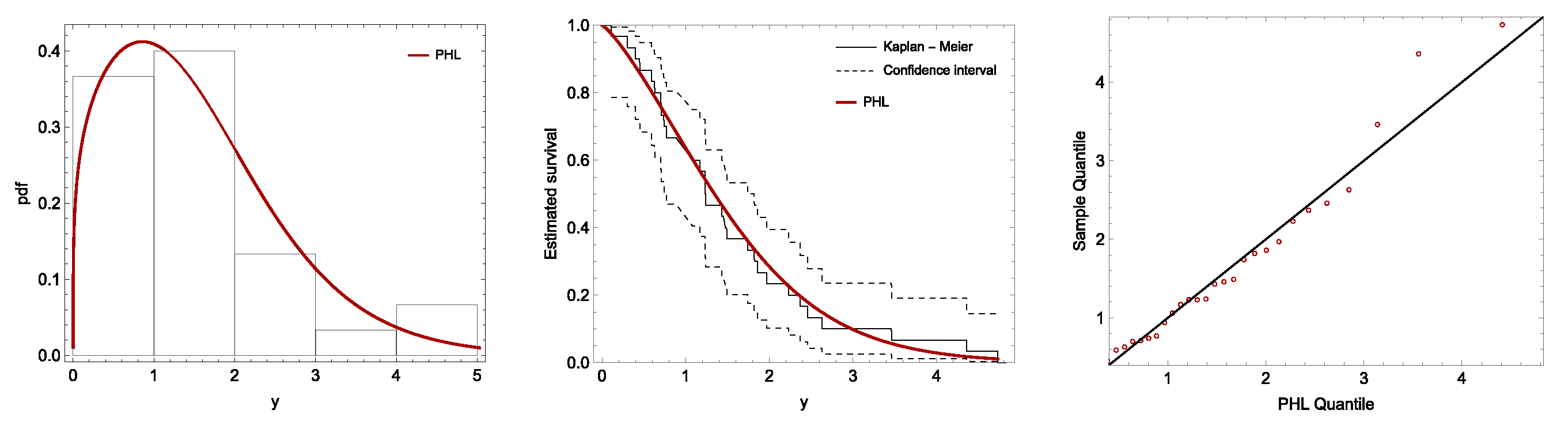
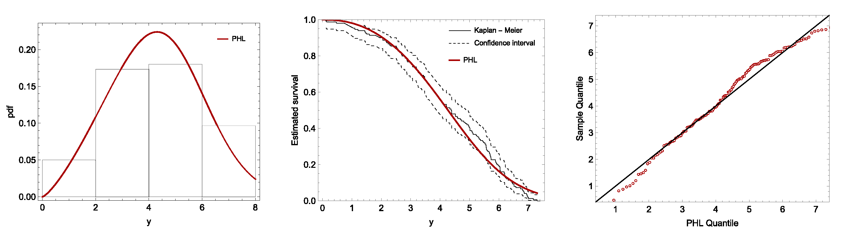
To further illustrate the applicability of the proposed model, we analyzed three different datasets under SSPALT. The analysis demonstrated the impact of applying the ATIIPC scheme on the predetermined duration of the experiment and the necessary adjustments to the censoring scheme. Furthermore, we successfully determined the optimal stress change times for each dataset. The findings confirm that the PHL distribution under complex experimental conditions, such as the SSPALT model with ATIIPC, provides a flexible and efficient framework.

While this study explores the SSPALT model’s effectiveness under the PHL distribution and ATIIPC scheme, several limitations should be noted. The analysis assumes the PHL distribution for lifetimes, and extending the model to other distributions could enhance its applicability. The optimal stress change time $\tau$ is determined numerically due to the lack of closed-form solutions, and future work could explore approximate analytical methods for improved computational efficiency. Additionally, the robustness of the model under varying levels of censoring, small sample sizes, and alternative prior assumptions in the Bayesian framework remains an area for further investigation. Expanding the study to adaptive stress-testing schemes and real-time monitoring could also provide more practical insights. Handling the inclusion of covariates, such as environmental factors and material properties, into the SSPALT model to study the effect of external variables on lifetimes is another open area. Lastly, validating the proposed methods across diverse real-world datasets and industries will further demonstrate their generalization and reliability.