Fatigue Detection Algorithm for Nuclear Power Plant Operators Based on Random Forest and Back Propagation Neural Networks

Abstract

This article proposes a fatigue detection algorithm for nuclear power plant control room operators based on random forest and BP neural networks, specifically targeting the control room scenario. This algorithm is capable of detecting fatigue-related operations in a timely manner, which is crucial for ensuring the safe operation of nuclear power plants. First, the random forest algorithm is used to classify the feature data according to different scenarios. Second, the data are distributed to different back propagation neural networks for prediction based on the scenario. Finally, experimental validation is conducted using a reactor simulation system. The results show that the algorithm achieves a recognition accuracy of 0.82, an accuracy of 0.69, a recall rate of 0.64, and an F1-Score of 0.66, indicating that the proposed algorithm has practical value for detecting operator fatigue in nuclear power plants. Compared to physiological data-based detection methods, it is simple, convenient, cost-effective, and does not interfere with operators.

1. Introduction

Throughout the 21st century, nuclear power has gradually become an indispensable part of the global energy system. According to the data from the International Atomic Energy Agency (IAEA) Power Reactor Information System, as of May 2024, there are 416 operable nuclear power reactors around the world, with a total net installed capacity of 374,597 megawatts (MWe), and nuclear power accounts for about 10% of the global total power generation. Therefore, attention to nuclear power operation is particularly important [1]. Research shows that human factors account for more than half of the major events and accidents in nuclear power plants. The Three Mile Island and Chernobyl nuclear power plant accidents that shocked the world clearly show that human factors are the main cause of serious accidents [2]. Operator fatigue is not uncommon. When operators are tired, they may not be able to make correct decisions in time, potentially leading to accidents. Therefore, research on the fatigue status of nuclear power plant operators is of great significance in ensuring nuclear power safety.

At present, there are three main objective detection methods for operator fatigue:

1.

Detection based on physiological data, such as EEG signals [3], ECG signals [4], etc. This method can accurately reflect the real-time state of the operator, but it usually requires special equipment which the operator needs to wear when testing, which can affect the operator’s ability to perform tasks, while the price of this equipment is high;

2.

Detection based on operator features, such as facial features [5,6,7], eye movement data [8], eye features [9], etc. This method is based on image detection technology. Image recognition technology usually relies on a camera with a fixed angle. When an operator works, they not only need to sit at the console for operation purposes, but also may need to walk, communicate with colleagues, check equipment, operate other control systems, etc. Once the operator leaves the monitoring range of the camera, this method will not be effective;

3.

Detection based on operating behavior characteristics, such as operating speed, amplitude, etc. This method can analyze the difference in operating characteristics under normal and fatigue conditions and build a discrimination model for detection [10,11].

The third method has no impact on the operator and incurs a lower cost. It does not need the operator to face the camera or keep their face unobstructed, nor does it need to consider the impact of light changes on the results of facial feature recognition. It only needs the operator to perform an operation to judge their fatigue state. It can work stably in all cases and has strong robustness. It can be integrated into the operating system. The fatigue discrimination model is essentially a classification algorithm which inputs the operating behavior characteristics of the operator and outputs the fatigue state of the operator. For classification tasks, the most common methods are logical regression, support vector machine, random forest, neural networks, etc. At the same time, the operator’s behavior is very complex and nonlinear, and the traditional linear method struggles to accurately describe this behavior. For this nonlinear classification task, BP neural networks are widely used and show good performance [12,13,14].

In this paper, the third scheme is adopted and a fatigue detection algorithm for nuclear power plant operators is proposed by comprehensively analyzing the characteristics of operators’ operation behavior. Compared with the traditional fatigue detection algorithm based on personnel’s facial features, this method uses the operators’ operation behavior characteristics as the judgment basis to avoid the algorithm failure caused by operators leaving the camera monitoring range or other factors (such as operators wearing masks and goggles or there being insufficient light). This method combines the random forest algorithm and BP neural networks to effectively detect the fatigue state of operators, demonstrating good performance in various working scenarios of nuclear power plants and effectively avoiding the occurrence of accidents.

The structure of this paper is as follows: Section 2 introduces the overall structure of the fatigue detection model, introduces the random forest algorithm and BP neural network, and makes some modifications to the algorithm according to the task requirements to make it more suitable for nuclear power scenarios. Section 3 introduces the training process of the model and verifies the performance of the model. Finally, Section 4 summarizes this paper and puts forward the directions for improvement in the future.

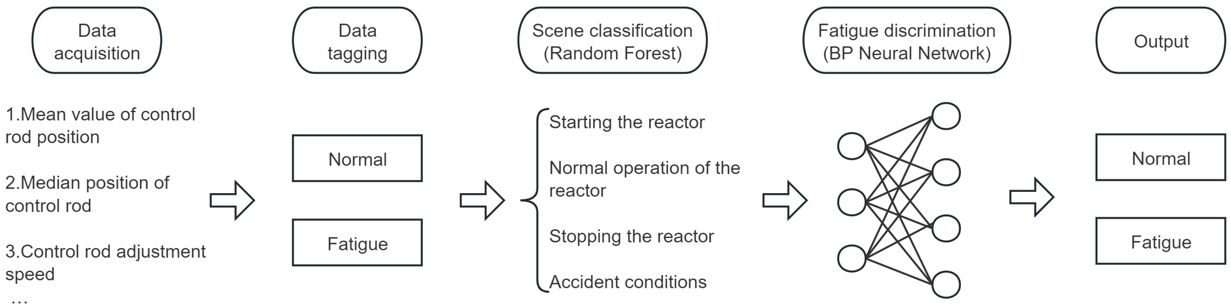
2. Algorithm Construction

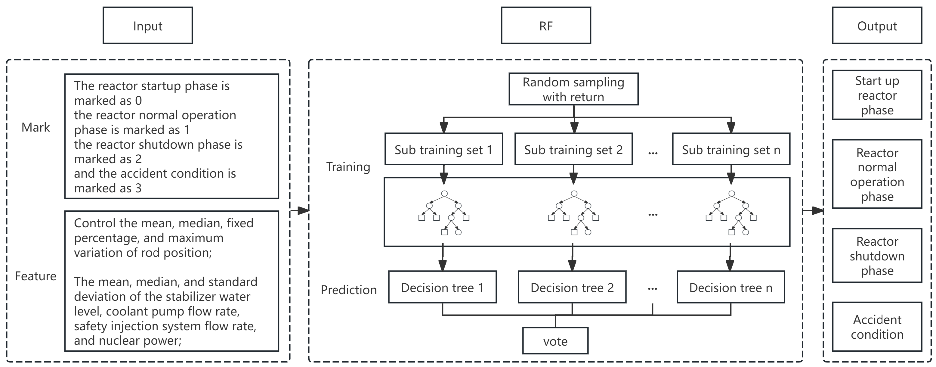
The fatigue detection algorithm is essentially a binary classification algorithm. During the training process, the classification algorithm typically seeks an “equilibrium state”, which is usually globally optimal but not necessarily locally optimal. Since the daily tasks of nuclear power plants involve four main scenarios, namely starting the reactor, the normal operation of the reactor, stopping the reactor, and accident conditions, the operating characteristics of the operator in each scenario do not always align with the reactor’s parameter changes [15]. Directly feeding data from all scenarios into a single neural network model may lead to poor adaptability of the model to different scenarios, which would affect the overall prediction accuracy. Therefore, it is necessary to first classify the working scenarios of the nuclear power plant and then use corresponding neural networks for prediction in each scenario. This approach allows the prediction result to be globally optimal while maintaining optimality within each category. Consequently, the model in this article classifies the data twice. The first classification step distinguishes the current scenario based on its features. According to the different scenarios, the appropriate classification algorithm is then used to detect the fatigue state of personnel.

Common classification algorithms include neural networks [16,17,18], polynomial logistic regression [19,20], support vector machines [21,22], random forest, etc., all of which offer high accuracy. However, the random forest algorithm has some unique advantages [23,24,25,26,27,28]: it is robust to noise and outliers in the dataset. Random forest can calculate the anomaly score of each data point (based on the degree of isolation of the data point in different trees), and the points with high scores are considered outliers. Since some feature data in this task, such as kernel power and control stick position, are constantly changing, binning is chosen as an outlier handling method. The data are divided into multiple intervals, and the median within each interval replaces the outliers. Additionally, random forest can automatically select appropriate features for classification tasks [29] without requiring additional operations. Therefore, this article adopts the random forest algorithm for scene classification.

There are many neural networks suitable for classification tasks when selecting fatigue detection models, such as BP neural networks, convolutional neural networks, and recurrent neural networks. BP neural networks are good at processing structured data (such as tables, feature vectors, etc.), convolutional neural networks perform well in image classification and are suitable for processing high-dimensional data, while recurrent neural networks excel in processing sequence data and capturing temporal dependencies. These classification algorithms have different applicable scenarios. Due to the low-dimensional and structured nature of the operator’s operation data, convolutional neural networks are not suitable for this task. Recurrent neural networks are effective for time-series data, but according to comparative experiments, they perform best for specific tasks and their performance significantly decreases when operators handle multiple tasks. BP neural networks, on the other hand, offer stable and good performance across all tasks. Considering the working environment of nuclear power plants, where operators not only handle specific tasks but sometimes need to deal with emergencies, a BP neural network with stable performance in any situation is a more suitable choice.

2.1. Random Forest

Random forest [30] (RF) is an ensemble learning method proposed by Breiman in 2001. A random forest consists of multiple decision trees, which are built by generating multiple training sets through random sampling with replacement from the original dataset. Each training set is then used to construct a decision tree, and these trees are grouped together to form a forest. The final output is determined by voting among the multiple decision trees. The specific steps are as follows:

1.

Randomly select n samples from the original dataset using the bootstrapping method to generate a training set;

2.

Randomly select k features ($k=\sqrt{m}$) from all m features as the division basis of the decision tree node to reduce over fitting and improve generalization ability;

3.

Establish a decision tree based on the selected training set and feature set;

4.

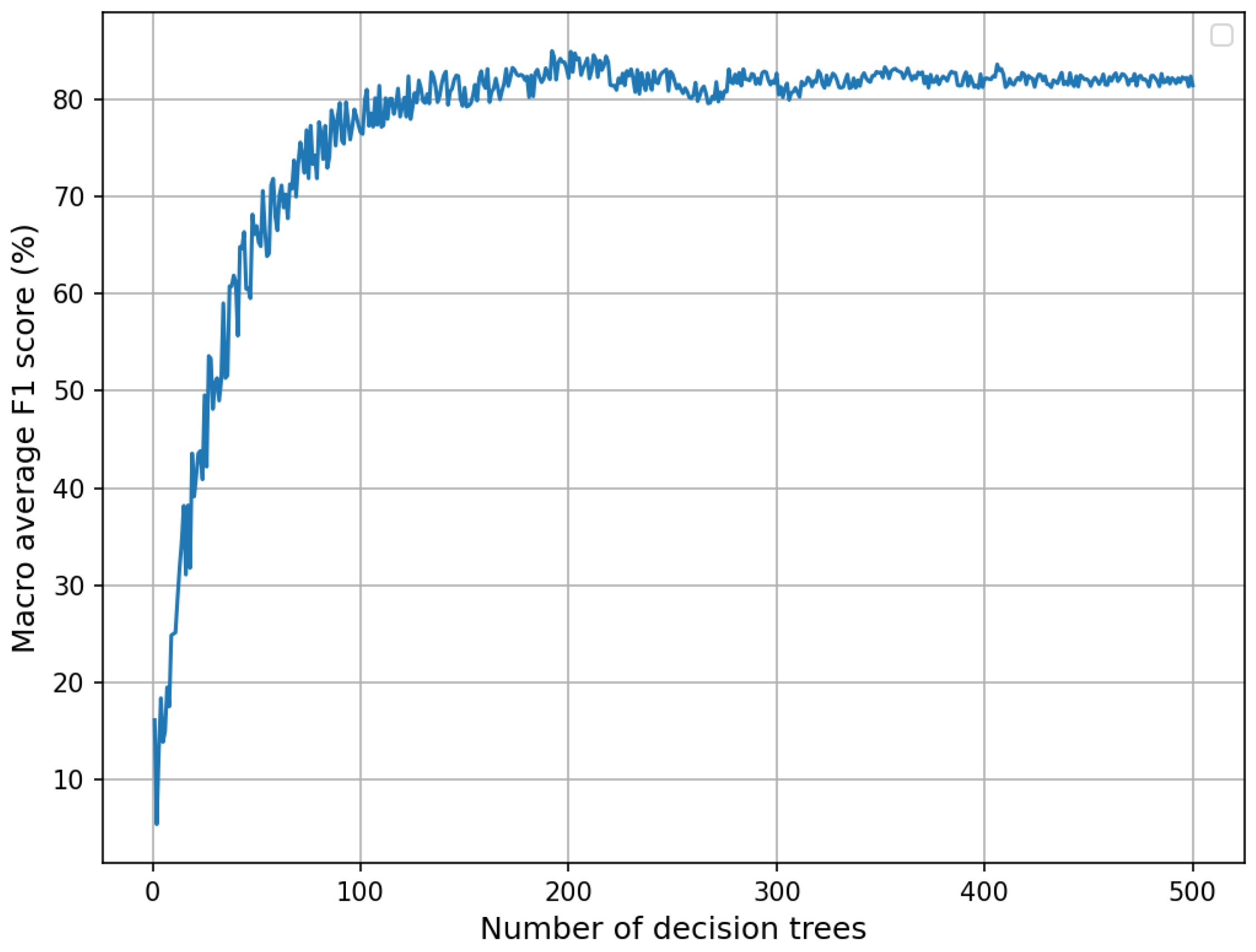
Repeat steps (1) to (3) to generate multiple decision trees, and control the size and performance of the random forest by setting the number of decision trees. The training process of each tree is recursive, starting from the root node to select the optimal splitting characteristics, and continue splitting at each child node until the stop conditions (such as maximum depth, minimum number of samples, etc.) are met;

5.

For a new data sample, predict on each decision tree and vote to determine the final result. The voting method is as follows, where mode refers to the category that gets the most votes and ${\widehat{y}}_n$ represents the prediction result of the nth decision tree.

$$\widehat{y}=\mathrm{mode}({\widehat{y}}_1,{\widehat{y}}_2,\dots ,{\widehat{y}}_n)$$

(1)

The goal of the decision tree is to split the dataset into subsets with increasing purity. For classification tasks, this paper uses the Gini coefficient [31] to measure the purity of each node. The specific calculation method is as follows:

$$G_j=1-\sum _{k=1}^K{p}_k^2$$

(2)

where $p_k$ is the proportion of samples with category k in node j and K is the number of categories. The smaller the $G_j$, the purer the node. If the node is not pure enough, select the feature with high importance to split. The calculation method of feature importance is as follows:

$$\mathrm{Importance}\left(f_k\right)={\displaystyle \frac{1}{B}}\sum _{b=1}^B\sum _{j\in {\mathrm{nodes}}_b}\Delta \mathrm{Impurity}\left(f_k\right)$$

(3)

$$\Delta \mathrm{Impurity}\left(f_k\right)=G_j\left(\mathrm{before}\right)-G_j\left(\mathrm{after}\right)$$

(4)

where $\mathrm{Importance}\left(f_k\right)$ indicates the importance of the feature $f_x$, B indicates the total number of decision trees, and ${\mathrm{nodes}}_b$ represents all nodes in the b-th tree. $G_j\left(\mathrm{before}\right)$ and $G_j\left(\mathrm{after}\right)$ are the purity before and after node splitting.

This article implements random forest based on the Scikit-learn (v1.2.2) library in Python (v3.9) and uses the Optimal Binning library to perform decision tree binning. Random forest can find the most suitable splitting points through recursive segmentation and can automatically handle outliers, improving robustness. Hyperparameters are determined using a grid search. The input data consist of the operator’s operational data. During training, the data are labeled: the reactor startup phase is marked as 0; the reactor normal operation phase is marked as 1; the reactor shutdown phase is marked as 2; and the accident condition is marked as 3. After training, the random forest reads the dataset and automatically selects segmentation points based on the Gini coefficient to construct decision trees. These trees vote to determine the current work scenario and send the input data to the corresponding neural network for prediction. The specific model structure of the random forest is shown in Figure 1.

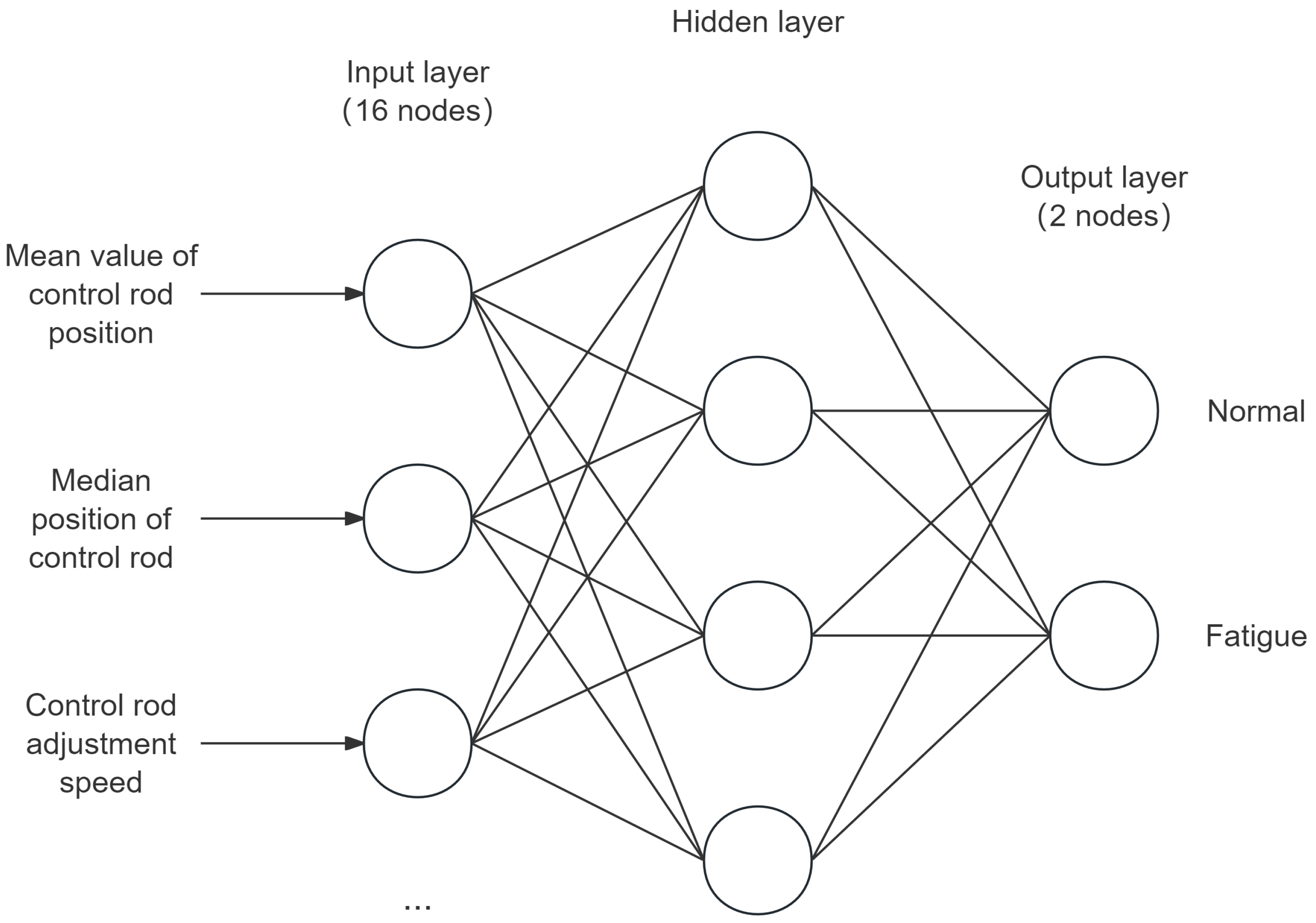
2.2. BP Neural Network

The back propagation (BP) neural network [32] is a multi-layer perceptron network, proposed by Rumelhart, Hinton, and Williams in 1986. It has strong nonlinear mapping ability and is suitable for handling complex classification problems. The network structure mainly includes an input layer, hidden layers, and an output layer [33]. The BP neural network can automatically extract the rules between input and output data and put the learning content in the network weight. It has strong nonlinear mapping ability, especially in structured data [34]. This article constructs a 16-8-2 neural network model based on the TensorFlow(v2.8.0) library in Python, where the 16 input nodes correspond to 16 feature variables and the 2 output nodes represent “normal” and “fatigue” states, respectively. The number of hidden layer nodes is compared and experimentally determined, and eight nodes is a more suitable number, being able to extract complex feature combinations, ensure model performance, and avoid overfitting problems. This structure is shown in Figure 2.

The commonly used activation functions for hidden layers include tansig, sigmoid, Leaky ReLU, etc. Due to the operator’s positive and negative operation data on the device, such as raising or lowering the control rod by 5 cm, Leaky ReLU allows negative input, but has low sensitivity to negative values, while tansig is sensitive to both positive and negative values, especially when the input is close to 0, the gradient is large, and the ability to capture the operator’s fine operations is stronger. After comparative experiments, tansig has been verified to perform well with regard to performance and convergence speed. Therefore, tansig (Tan sigmoid, hyperbolic tangent S-shaped activation function) is used as the neuron activation function for hidden layers

As it is a binary classification task, the output layer uses logsig (Log sigmoid) as the neuron activation function.

The back propagation algorithm [35] is used to adjust the weight of the neural network. For the binary classification problem, the most commonly used loss function is cross entropy loss. The calculation formula is as follows, where the actual value is $y_i$ and the predicted value is ${\widehat{y}}_i$.

$$L=-{\displaystyle \frac{1}{N}}\sum _{i=1}^N[y_{i}log\left({\widehat{y}}_i\right)+(1-y_i)log(1-{\widehat{y}}_i)]$$

(5)

Due to the non-linear nature of the operator’s operations, the RMSProp (Root Mean Square Propagation) algorithm can adapt well to such non-stationary data. However, the operational data may contain operator errors. The gradient normalization of the RMSprop algorithm can effectively suppress the influence of noise and improve the model’s generalization ability. By using backpropagation to update gradients and RMSProp optimization algorithm to update weights and biases, the derivation process is as follows:

$${\displaystyle \frac{\partial L}{\partial z^{\left(t\right)}}}={\displaystyle \frac{\partial L}{\partial a^{\left(t\right)}}}·{\displaystyle \frac{\partial a^{\left(t\right)}}{\partial z^{\left(t\right)}}}$$

(6)

$${\displaystyle \frac{\partial L}{\partial a^{\left(t\right)}}}=a^{\left(t\right)}-y$$

(7)

Hidden layer (the activation function is tansig):

$${\displaystyle \frac{\partial a^{\left(t\right)}}{\partial z^{\left(t\right)}}}=1-{\left(a^{\left(t\right)}\right)}^2$$

(8)

Output layer (the activation function is logsig):

$${\displaystyle \frac{\partial a^{\left(t\right)}}{\partial z^{\left(t\right)}}}=a^{\left(t\right)}(1-a^{\left(t\right)})$$

(9)

Multiply them to obtain the gradient of the hidden layer and the output layer. Use the RMSProp algorithm to adaptively adjust the weight and offset as follows:

$$G_t=\gamma G_{t-1}+\left(1-\gamma \right){\left({\displaystyle \frac{\partial L}{\partial z^{\left(t\right)}}}\right)}^2$$

(10)

$${\omega }_t={\omega }_{t-1}-{\displaystyle \frac{\eta }{\sqrt{G_t+ϵ}}}·{\displaystyle \frac{\partial L}{\partial z^{\left(t\right)}}}$$

(11)

$$b_t=b_{t-1}-{\displaystyle \frac{\eta }{\sqrt{G_t+ϵ}}}·{\displaystyle \frac{\partial L}{\partial z^{\left(t\right)}}}$$

(12)

In this formula, $\eta$ is the global learning rate, set to 0.9, and $ϵ$ is a small constant, set to ${10}^{-8}$, which is used to prevent dividing by zero. Compared with a fixed learning rate, the use of the adaptive learning rate can effectively avoid overfitting and local optimal solutions, improve the generalization ability of the model, and also improve the convergence speed. When the output of the loss function gradually decreases to a flat level, the training is terminated.

Based on the characteristics of the random forest algorithm and the BP neural network, the main steps of the construction and fatigue detection algorithm for nuclear power plant operators are as follows: first, extract the characteristics of operators’ operation behavior. In order to improve the accuracy, the random forest algorithm is used to classify the data. Then, send the data of different scenarios into the corresponding BP neural network for judgment. The overall framework of the algorithm is shown in Figure 3.

3. Experiment

3.1. Data Acquisition

This article used the CGN ACPR50S simulation reactor system for operational simulation experiments, recruiting a total of 12 participants aged between 28 and 35, all of whom are experienced nuclear power plant operators. The participants complete tasks such as starting the reactor, normal operation, shutting down the reactor, and handling accidents as required. Each participant participated in two experiments, with a minimum 24 h interval between each experiment to ensure that they were in a non-fatigued state before each experiment.

The simulation reactor system records reactor-related data every second, including date and time, experiment number, task name, operator name, nuclear power, primary loop pressure, control rod position, coolant system flow rate, safety injection system flow rate, and more. During the experiment, participants followed the corresponding task protocol. Since all experimental data were exported from the simulation system, there was no issue of missing data. Additionally, outliers were handled using binning in random forest, and the activation function for the hidden layer of the neural network was tansig. Normalization is not well-suited to tansig, so standardization was chosen as the data preprocessing method. Standardization can eliminate dimensional differences, improve model fairness, and enhance both training efficiency and performance.

To assess the status of the subjects, a self-assessment was conducted after each task (approximately every 15 min), and the evaluation results were divided into two categories: normal and fatigued. When the subject felt fatigued, they continued to perform the task at least once before deciding whether to continue the experiment independently. Over time, the fatigue status of the subjects changed and the number of fatigued individuals over time is shown in

Table 1. The change in the number of fatigued individuals ove time.

Time Slot/min	Number of Fatigued People
0–15	0
15–30	1
30–45	2
45–60	5
60–75	3
75–90	1

.

Since the fatigue state was detected every 15 min, it was not possible to accurately determine the subjects’ working states during the transition between normal and fatigue states; therefore, the data from this period were excluded. Additionally, not all behaviors after fatigue was reported by the subjects could be classified as fatigue work. The classification was made by combining operational videos, images, and the subjects’ self-assessments. A one-minute time window was used to intercept and label data as either fatigued or normal work. In total, 284 valid samples were collected, including 188 normal work samples and 96 fatigue work samples, with fatigure work samples representing 33.8% of the samples. There are four operation scenarios in the experiment: the startup of reactor, the normal operation of reactor, the shutdown of reactor, and accident conditions. The number of samples in different scenarios is shown in

Table 2. Number of samples in different scenarios.

Scenario	Number of Samples in the Normal State	Number of Samples in the Fatigued State
Starting the reactor	43	21
Normal operation of the reactor	51	22
Stopping the reactor	45	22
Accident conditions	49	31

.

It can be observed that the normal state samples in the dataset significantly outnumbered the fatigue state samples. Using standard cross-entropy loss would cause the model to favor the normal state and ignore the fatigue state. To address this issue, we applied weights to the cross-entropy loss function. The weighted loss function is as follows, where ${\omega }_0$ and ${\omega }_1$ are weights, set to 2 and 1, respectively, to ensure that both states receive equal attention during training.

$$L=-{\displaystyle \frac{1}{N}}\sum _{i=1}^N[{\omega }_1{y}_{i}log\left({\widehat{y}}_i\right)+{\omega }_0(1-y_i)log(1-{\widehat{y}}_i)]$$

(13)

The gradient calculation formula then becomes

$${\displaystyle \frac{\partial L}{\partial z^{\left(t\right)}}}=(\omega 1y^{\left(t\right)}+\omega 0(1-y^{\left(t\right)}))·{\displaystyle \frac{\partial L}{\partial a^{\left(t\right)}}}·{\displaystyle \frac{\partial a^{\left(t\right)}}{\partial z^{\left(t\right)}}}$$

(14)

3.2. Feature Extraction

In the reactor startup phase, the operator gradually raises the control rod, which is characterized by a small operating range, a fixed and moderate operating frequency, and a steady increase in nuclear power. During the normal operation of the reactor, the operator adjusts the control rod position according to the power generation demand, characterized by a small operating range, a low operating frequency, and generally stable nuclear power. In the reactor shutdown phase, the operator gradually lowers the control rod, which is characterized by a medium operating range, a fixed and fast operating frequency, and a steady reduction in nuclear power. In accident conditions, the operator quickly inserts the control rod into the reactor core to stop the nuclear reaction as quickly as possible, which is characterized by a large operating range, one-step operation, and a rapid reduction in nuclear power. The reaction speed and information processing ability of operators are affected under fatigue, leading to notable differences between fatigued and normal operators, with the main symptoms being increased operation delays and frequent adjustments.

The typical operation waveform for the operator controlling the rod position during the reactor startup task under both normal and fatigue conditions is shown in Figure 4. Figure 4a shows the control rod position waveform under the normal state of the operator. It can be observed that the operator moves the control rod with a relatively uniform frequency and accurate amplitude. Figure 4b shows the control rod position waveform under the fatigued state of the operator, where the operating amplitude is either too large or insufficient, the operating frequency increases, and delayed operations are observed.

The characteristics of control rod operations in these two cases can be described using the fixed percentage of the rod position, which measures the proportion of time the control rod position remains unchanged over a period. Generally speaking, the higher the fixed percentage of the control rod position, the more it indicates that the operator’s actions are precise, requiring fewer adjustments to the control rod, which reflects a good operational state. Since the reactor is a complex system with closely interconnected and inseparable components, it was necessary to collect operational data from all equipment that the operator must control on a daily basis in order to comprehensively evaluate the operator’s behavior. This includes control rods, stabilizers, coolant pumps, and safety injection systems. Additionally, nuclear power data were used to assist in the judgment, resulting in a total of 16 types of characteristic data.

1.

Control rod position: mean, median, fixed percentage, and maximum variation;

2.

Pressurizer water level: mean, median, and standard deviation;

3.

Coolant pump flow: mean, median, and standard deviation;

4.

Safety injection system flow: mean, median, and standard deviation;

5.

Nuclear power: mean, median, and standard deviation.

3.3. Feature Analysis

The 16 data features were obtained, and the relationship between each feature and drowsy driving can be indicated by the Pearson correlation coefficient. The Pearson correlation coefficient is an indicator used to measure the degree of linear correlation between two variables. It is defined as the ratio of the covariance between the two variables to the product of their standard deviations, as shown in Equation (15):

$${\rho }_{X,Y}={\displaystyle \frac{\mathrm{cov}(X,Y)}{{\sigma }_X{\sigma }_Y}}={\displaystyle \frac{E\left[(X-{\mu }_X)(Y-{\mu }_Y)\right]}{{\sigma }_X{\sigma }_Y}}$$

(15)

where $\rho$ represents the Pearson correlation coefficient; $\mathrm{cov}(X,Y)$ represents the covariance between X and Y; $\sigma$ represents the standard deviation of eigenvalue; and $\mu$ represents the mean value of characteristic values.

We obtained the most likely fatigue related features through correlation coefficients. By performing this calculation, the correlation coefficients between different operational characteristics and fatigue work could be obtained. Taking the start-up reactor scenario as an example, the correlation coefficients between each characteristic and fatigue state are detailed in

Table 3. Pearson correlation coefficient between different operational characteristics and fatigue work.

Feature	Pearson Correlation
Average value of control rod position	−0.21
Median of control rod position	−0.16
Control rod position fixed percentage	−0.33
Maximum value of control rod position change	0.16
Mean value of pressurizer water level	−0.15
Median of pressurizer water level	−0.29
Standard deviation of pressurizer water level	0.17
Average flow of coolant pump	−0.11
Coolant pump flow median	−0.14
Standard deviation of coolant pump flow	0.08
Mean flow of safety injection system	−0.05
Median flow of safety injection system	−0.08
Standard deviation of safety injection system flow	0.09
Average nuclear power	−0.08
Median nuclear power	−0.07
Standard deviation of nuclear power	0.08

. Among them, the correlation coefficient between the safety injection system and nuclear power is relatively low, because the safety injection system is mainly used to deal with accidents and is less used in other working conditions, while nuclear power data are mainly used to determine the current operating conditions. In the scenario of starting the reactor, the control rod position, stabilizer water level, coolant pump flow rate, safety injection system flow rate, and nuclear power all gradually increase. However, the operator experiences operational delays and inadequacies in the fatigue state, and the increases in various characteristic data are slower than normal. Therefore, the correlation coefficient between the mean and median and the fatigue state shows a negative value. Moreover, due to the operator’s tendency to frequently adjust various equipment in the fatigue state, the standard deviation of each type of characteristic data is positively correlated with the fatigue state. From the correlation coefficient between features and fatigue operation behavior, the correlation coefficient between each feature and the fatigue state is not high. The reason for this is that the reactor is a complex system, and in order to maintain the nuclear reaction within a controllable range, the operator needs to control multiple devices. Therefore, the operation data of a single device cannot directly reflect the fatigue state of the judgment personnel, and multiple features need to be jointly judged.

3.4. Model Construction and Verification

Due to class imbalance in the dataset, the ratio of fatigue samples to normal samples was 1:2. Therefore, K-fold cross validation was chosen as the training and validation method for the model. K-fold cross validation ensures that each subset maintains the sample proportions through stratified sampling. Compared to single partitioning, this method can significantly reduce bias caused by uneven data distribution, while also effectively improving data utilization. As personnel fatigue data were collected every 15 min in the experiment, the model requires at least 15 min of operational data to determine the operator’s fatigue status. Additionally, due to reactor lag, the operator’s actions take several minutes to manifest. A complete nuclear power task typically consists of several unit tasks, and completing the full task often takes several hours or even days. For example, the ACPR50S reactor used in this experiment takes 2 days to start and 1 day to shut down, so a 15 min interval is more suitable. This interval ensures the real-time performance of the model and avoids performance degradation caused by insufficient operational data. Due to the uneven distribution of sample labels, accuracy, recall, and precision were introduced to assist in the analysis [36]. Accuracy refers to the proportion of correctly predicted samples among all samples and is the most intuitive performance indicator. Recall refers to the proportion of correctly predicted positive samples among all actual positive samples. Precision refers to the proportion of actual positive samples among all predicted positive samples. Accuracy and recall are often interdependent. High accuracy indicates fewer false positives, but may miss some actual positive samples, while high recall improves the detection of positive samples but may increase false positives, thus reducing accuracy. Therefore, the F1-Score was introduced to comprehensively evaluate both accuracy and recall. The calculation methods for each evaluation metric are as follows:

$$\mathrm{Accuracy}={\displaystyle \frac{TP+TN}{TP+TN+FP+FN}}$$

(16)

$$\mathrm{Precision}={\displaystyle \frac{TP}{TP+FP}}$$

(17)

$$\mathrm{Recall}={\displaystyle \frac{TP}{TP+FN}}$$

(18)

$$\mathrm{F}1-\mathrm{Score}={\displaystyle \frac{2\times \mathrm{Precision}\times \mathrm{Recall}}{\mathrm{Precision}+\mathrm{Recall}}}$$

(19)

Figure 5 shows the variation in the macro-average F1-Score during the training process of the random forest algorithm as the decision tree depth changes. As the tree depth increases, the macro-average F1-Score rises rapidly. When the depth reaches 8, the increase in the macro-average F1-Score slows significantly and begins to converge. Further increasing the depth does not result in a noticeable improvement in the macro-average F1-Score. This suggests that, in the initial stage, increasing the decision tree depth enhances the model’s fitting ability and reduces errors. However, once the depth exceeds a certain threshold, further increases do not yield significant gains in accuracy. Therefore, the maximum decision tree depth was set to 12. Figure 6 shows the variation in the macro-average F1-Score during training as the number of decision trees changes. When the number of trees reaches 150, the macro-average F1-Score stabilizes, with the maximum value occurring at 193. Therefore, the number of decision trees was set to 200, which ensured model accuracy while avoiding unnecessary computational overheads.

The hyperparameters in the random forest algorithm were validated using a grid search (GS), with a detailed grid search focusing on the maximum depth and number of decision trees. The macro-average F1-Score was used as the evaluation metric. The specific results are shown in Figure 7. From the results, it can be seen that when the maximum decision tree depth is set to 12 and the number of decision trees is set to 200, the model performance reaches a good balance, indicating that the selection of these two hyperparameters is reasonable.

Table 4. Comprehensive performance of the random forest algorithm.

Scenario	Accuracy	Precision	Recall	F1-Score
Starting the reactor	0.87	0.85	0.84	0.84
Normal operation of the reactor	0.86	0.81	0.78	0.79
Stopping the reactor	0.88	0.82	0.86	0.84
Accident conditions	0.85	0.80	0.82	0.81
Macro-average	0.87	0.82	0.82	0.82

shows the classification performance metrics for the four operational scenarios of a nuclear power plant, demonstrating that the random forest algorithm can effectively classify each operational scenario and provide the data for the corresponding scenario’s neural network.

Data from different scenarios were used to train the corresponding neural networks, and the loss curves for each scenario are shown in Figure 8. From the training loss curves, it can be seen that after 100 epochs, the losses for all scenarios stabilize, achieving high recognition accuracy. The specific performance metrics of the neural networks for each scenario are shown in

Table 5. Comprehensive performance of the neural network.

Scenario	Accuracy	Precision	Recall	F1-Score
Starting the reactor	0.92	0.83	0.81	0.82
Normal operation of the reactor	0.84	0.69	0.59	0.64
Stopping the reactor	0.90	0.82	0.80	0.81
Accident conditions	0.88	0.73	0.65	0.69

. Among them, in the scenarios of starting and stopping the reactor, the neural network performs well across all aspects. However, the performance is slightly weaker in the scenario of normal reactor operation. The reason for this is that in the scenarios of starting and stopping the reactor, the operator’s actions are more intensive and the features are more distinct, making it easier for the neural network to recognize and differentiate the operator’s working state. On the other hand, in the normal reactor operation scenario, the reactor state is relatively stable, the operator’s action frequency significantly decreases, and the range of actions is smaller. This results in relatively smooth feature variations during this stage, which do not provide sufficient dynamic information for the neural network, leading to weaker performance in this scenario.

By combining the two models, a complete fatigue detection model for nuclear power plant operators is obtained.

3.5. Model Comprehensive Performance Evaluation

In order to comprehensively evaluate the performance of the model, the model was embedded into the reactor simulation system. The experimenters randomly set task objectives, and the operator executed the task on the reactor simulation system. In order to verify the generalization ability of the model, this task was not included in the training data, and an additional 8 operators were recruited on the basis of the original 12 operators, for a total of 20 people to participate in this experiment. Before the experiment, we ensured that the operators received sufficient rest, and the interval between the two experiments exceeded 24 h. When the operator felt tired, they reported as such and continued to perform the task for 15 min. The experimenter recorded the moment when the operator felt tired and the moment when the model judged that the they were tired. If the interval between the two did not exceed 15 min, or if neither the operator nor the model reported fatigue until the task was completed, it was considered that the model had successfully detected the operator’s fatigue state.

A total of 100 experiments were conducted, and the experimental results are shown in

Table 6. Experimental result.

	Actual Fatigue	Actually Not Fatigue
Predicting fatigue	18	8
Predicted not fatigued	10	64

. The calculated accuracy is 0.82, the precision is 0.69, the recall rate is 0.64, and the F1-Score is 0.66. This indicates that the method proposed in this paper can accurately detect the working status of operators and has the characteristics of wide applicability, strong stability, no interference with personnel, and low cost.

Using the same experimental data, logistic regression, support vector machine, and a unclassified neural network were trained. Logistic regression has the fastest training speed, support vector machine has a slower training speed, and the unclassified neural network had a medium training speed due to GPU acceleration. In this paper, the algorithm needed to train two components, the random forest algorithm and the BP neural network, so it had the slowest training speed. In terms of scalability, logistic regression can process large-scale data through online learning with stochastic gradient descent (SGD), but its model is simple and has limited expressive power. The training complexity of the support vector machine is relatively high, causing it to struggle to process large-scale data directly, making it more suitable for small- to medium-sized classification tasks. Both unclassified neural networks and the algorithm proposed in this paper can handle large-scale data through hardware acceleration, and have strong generalization capabilities, allowing them to express complex tasks. The logistic regression, support vector machine, and unclassified neural network algorithms were applied to the data in this experiment. The experimental results were compared with those for the method proposed in this paper, and the results are shown in Figure 9. It can be seen that the neural network algorithm after scene classification performs well with regard to accuracy, recall, precision, and F1-Score.

4. Summary

4.1. Conclusions

This article collects operational data from a simulated reactor system and extracts 16 characteristic data points. Using the random forest algorithm, the data are classified into four scenarios: starting the reactor, normal reactor operation, reactor shutdown, and accident conditions. The classified data are then sent to the corresponding neural network to determine the operator’s work status.

The results from the reactor operation experiments using the simulated reactor system show that the operator fatigue detection algorithm based on random forest and BP neural networks outperforms the logistic regression, support vector machine, and unclassified neural network algorithms in terms of accuracy, recall, precision, and F1-Score in identifying the operator’s work status. Additionally, the detection process does not interfere with the operator. The proposed fatigue detection algorithm has practical significance for detecting operator fatigue in nuclear power plants.

4.2. Future Directions

Although the operator fatigue detection method for nuclear power plants proposed in this study, based on the random forest and BP neural network algorithms, achieved significant results in terms of accuracy, recall, precision, and F1-Score, there are still areas that warrant further exploration and improvement. Future research could focus on the following directions:

1.

In this study, fatigue is determined based on the operator’s subjective feelings. Future work could incorporate additional fatigue detection methods, such as physiological data, eye movement data, and the NASA-TLX scale, to more accurately assess whether the operator is fatigued. This would improve the dataset’s accuracy and further enhance the predictive performance of the fatigue detection algorithm;

2.

In addition to operational behavior features, future research could explore integrating image-recognition-based fatigue detection algorithms, combining both approaches to further improve the accuracy of fatigue detection;

3.

Although the model demonstrates high prediction accuracy, its interpretability is relatively limited. In future work, methods to improve model interpretability, such as ACT-R, SHAP, or LIME, could be employed to analyze the model’s decision-making process, helping operators understand which behaviors or actions are most likely to lead to fatigue.

References

1. Chen, D. Nuclear Energy and Nuclear Safety: Analysis and Reflection on the Fukushima Nuclear Accident in Japan. J. Nanjing Univ. Aeronaut. Astronaut. 2012, 44, 597–602. [Google Scholar] [CrossRef]
2. Fang, X.; Zhao, B. Selection and Experiment of Cognitive Reliability Research Model for Nuclear Power Plant Operators. Nucl. Sci. Eng. 2000, 145, 18–24. [Google Scholar]
3. Li, L.; Qing, T.; Xiang, X.; Tang, Y.Q.; Fu, J.H.; Chen, J. Feasibility Study on Fatigue Evaluation of Nuclear Power Plant Operators Using EEG Technology. Sci. Technol. Innov. Appl. 2024, 14, 24–27. [Google Scholar] [CrossRef]
4. Dong, Z.; Sun, S.; Wu, Q.; Xu, J.F. Study on the Correlation between Heart Rate Variability and Driver Fatigue. J. Zhejiang Univ. (Eng. Ed.) 2010, 44, 46–50. [Google Scholar]
5. Geng, L.; Yuan, F.; Xiao, Z.; Zhang, F.; Wu, J.; Li, Y.L. Driver Fatigue Detection Based on Facial Behavior Analysis. Comput. Eng. 2018, 44, 274–279. [Google Scholar]
6. Hijji, M.; Yar, H.; Ullah, F.U.M.; Alwakeel, M.M.; Harrabi, R.; Aradah, F.; Cheikh, F.A.; Muhammad, K.; Sajjad, M. FADS: An Intelligent Fatigue and Age Detection System. Mathematics 2023, 11, 1174. [Google Scholar] [CrossRef]
7. Wang, Y.; He, Z.; Wang, L. Truck Driver Fatigue Detection Based on Video Sequences in Open-Pit Mines. Mathematics 2021, 9, 2908. [Google Scholar] [CrossRef]
8. Dai, L.; Zhang, M.; Li, Y.; Ma, L.; Han, X.Y.; Chen, X.; Li, P.C. Research on Operator Cognitive Load in Nuclear Power Plant Digital Control Rooms Based on Gaze Entropy. J. Saf. Environ. Eng. 2023, 23, 1985–1993. [Google Scholar]
9. Xiang, Y.; Hu, R.; Xu, Y.; Hsu, C.-Y.; Du, C. Gaussian Weighted Eye State Determination for Driving Fatigue Detection. Mathematics 2023, 11, 2101. [Google Scholar] [CrossRef]
10. Zhang, X.; Cheng, B.; Feng, R. Real-time Driver Fatigue Detection Method Based on Steering Wheel Operation. J. Tsinghua Univ. (Nat. Sci. Ed.) 2010, 50, 1072–1076+1081. [Google Scholar] [CrossRef]
11. Jia, L. Study on Fatigue Driving Detection Method Based on Steering Wheel Operation Features in Real Vehicles. Ph.D. Thesis, Tsinghua University, Beijing, China, 2017. [Google Scholar]
12. Li, Z.; Ma, Q. Application of BP Neural Network in Nonlinear Classification Problems. Comput. Intell. Neurosci. 2022, 2154050. [Google Scholar]
13. Yang, Y.; Zhang, J. A New Backpropagation Neural Network Algorithm for Classifying Nonlinear Data. Neural Process. Lett. 2021, 53, 1325–1339. [Google Scholar]
14. Chen, X.; Wang, Y. Optimized BP Neural Network for Nonlinear Classification Applications. J. Artif. Intell. Neural Netw. 2023, 1–10. [Google Scholar]
15. Zhang, Y. The Working Principles and Development Trends of Nuclear Power Plants. Equip. Mach. 2010, 4, 2–7. [Google Scholar]
16. Qi, D.; Kang, J. Design of BP Neural Network. Comput. Eng. Des. 1998, 2, 47–49. [Google Scholar] [CrossRef]
17. Shukla, A.; Patel, R. A Comprehensive Review on Backpropagation Neural Network (BPNN) and Its Variants. Neural Comput. Appl. 2021, 33, 14297–14318. [Google Scholar]
18. Jain, P.; Kumar, P. Exploring the Backpropagation Neural Network for Classification and Optimization Tasks. Comput. Intell. Neurosci. 2022, 9231845. [Google Scholar]
19. Hu, J.; Tan, K.; Wu, L. An Improved Polynomial Logistic Regression Method for Hyperspectral Image Classification. Remote. Sens. Technol. Appl. 2015, 30, 135–139. [Google Scholar]
20. Tan, X.; Wu, Y.; Yuan, Z.; Li, J. Parallel Computing Optimization of Lagrange Polynomial Logistic Regression Classification Algorithm. Remote Sens. Inf. 2016, 31, 96–101. [Google Scholar]
21. Ding, S.; Qi, B.; Tan, H. A Review of Support Vector Machine Theory and Algorithms. J. Univ. Electron. Sci. Technol. 2011, 40, 2–10. [Google Scholar]
22. Zhang, X. On Statistical Learning Theory and Support Vector Machines. Acta Autom. Sinica 2000, 1, 36–46. [Google Scholar] [CrossRef]
23. Fang, N.; Wu, J.B.; Zhu, J.P.; Xie, B.C. A Review of Random Forest Methods. Stat. Inf. Forum 2011, 26, 32–38. [Google Scholar]
24. Fernández-Delgado, M.; Cernadas, E.; Barro, S.; Amorim, D. Do We Need Hundreds of Classifiers to Solve Real World Classification Problems? J. Mach. Learn. Res. 2014, 15, 3133–3181. [Google Scholar]
25. Caruana, R.; Niculescu-Mizil, A. An Empirical Comparison of Supervised Learning Algorithms. In Proceedings of the 23rd International Conference on Machine Learning, Pittsburgh, PA, USA, 25–29 June 2006; pp. 161–168. [Google Scholar]
26. Li, Y.; Chen, W. A Comparative Performance Assessment of Ensemble Learning for Credit Scoring. Mathematics 2020, 8, 1756. [Google Scholar] [CrossRef]
27. Saito, T.; Rehmsmeier, M. Random Forests and Support Vector Machines: A Comparison of Advantages in Classification Tasks. Comput. Intell. 2021, 37, 823–840. [Google Scholar] [CrossRef]
28. Liaw, A.; Wiener, M. Random Forests: Classification and Regression. In Springer Handbook of Computational Intelligence; Springer: Berlin/Heidelberg, Germany, 2007; pp. 531–540. [Google Scholar]
29. Li, X. Application of Random Forest Model in Classification and Regression Analysis. Chin. J. Appl. Entomol. 2013, 50, 1190–1197. [Google Scholar]
30. Breiman, L. Random Forests. Mach. Learn. 2001, 45, 5–32. [Google Scholar] [CrossRef]
31. Liaw, A.; Wiener, M. Classification and Regression by randomForest. R News 2002, 2, 18–22. [Google Scholar]
32. Rumelhart, D.E.; Hinton, G.E.; Williams, R.J. Learning Representations by Back-propagating Errors. Nature 1986, 323, 533–536. [Google Scholar] [CrossRef]
33. Hecht-Nielsen, R. Theory of the Backpropagation Neural Network. In Proceedings of the International 1989 Joint Conference on Neural Networks, Washington, DC, USA, 18–22 June 1989; Academic Press: Cambridge, MA, USA, 1989; pp. 65–93. [Google Scholar]
34. Liu, X.; Pan, Y.; Yan, Y.; Wang, Y.; Zhou, P. Adaptive BP Network Prediction Method for Ground Surface Roughness with High-Dimensional Parameters. Mathematics 2022, 10, 2788. [Google Scholar] [CrossRef]
35. Rumelhart, D.E.; McClell, J.L.; PDP Research Group. Parallel Distributed Processing, Volume 1: Explorations in the Microstructure of Cognition: Foundations; The MIT Press: Cambridge, MA, USA, 1986. [Google Scholar]
36. Sokolova, M.; Lapalme, G. A Systematic Analysis of Performance Measures for Classification Tasks. Inf. Process. Manag. 2009, 45, 427–437. [Google Scholar] [CrossRef]
Figure 1. Schematic diagram of random forest structure.
Mathematics 13 00774 g001
Figure 2. Schematic diagram of BP neural network.
Mathematics 13 00774 g002
Figure 3. Overall framework of the algorithm.
Mathematics 13 00774 g003
Figure 4. Typical waveforms of control rod position in different states.
Mathematics 13 00774 g004
Figure 5. Relationship between macro-average F1-score and maximum depth of decision trees.
Mathematics 13 00774 g005
Figure 6. Relationship between macro-average F1 score and number of decision trees.
Mathematics 13 00774 g006
Figure 7. Grid search results.
Mathematics 13 00774 g007
Figure 8. Loss for each scenario.
Mathematics 13 00774 g008
Figure 9. Experimental results of different algorithms.
Mathematics 13 00774 g009