Abstract
Prior elicitation is an important issue in both subjective and objective Bayesian frameworks, where prior distributions impose certain information on parameters before data are observed. Caution is warranted when utilizing noninformative priors for hypothesis testing or model selection. Since noninformative priors are often improper, the Bayes factor, i.e., the ratio of two marginal distributions, is not properly determined due to unspecified constants contained in the Bayes factor. An adjusted Bayes factor using a data-splitting idea, which is called the intrinsic Bayes factor, can often be used as a default measure to circumvent this indeterminacy. On the other hand, if reasonable (possibly proper) called intrinsic priors are available, the intrinsic Bayes factor can be approximated by calculating the ordinary Bayes factor with intrinsic priors. Additionally, the concept of the integral prior, inspired by the generalized expected posterior prior, often serves to mitigate the uncertainty in traditional Bayes factors. Consequently, the Bayes factor derived from this approach can effectively approximate the conventional Bayes factor. In this article, we present default Bayesian procedures when testing the zero inflation parameter in a zero-inflated Poisson distribution. Approximation methods are used to derive intrinsic and integral priors for testing the zero inflation parameter. A Monte Carlo simulation study is carried out to demonstrate theoretical outcomes, and two real datasets are analyzed to support the results found in this paper.
Keywords:
asymptotic equivalence; integral prior; intrinsic Bayes factor; intrinsic prior; training sample; zero inflation MSC:
62-08; 62F15
1. Introduction
Discrete data have been analyzed across various fields, ranging from the social sciences, such as economics and management, to natural sciences, like ecology. Several distributions may be utilized in dealing with discrete data, among which the Poisson distribution is one of the most commonly used models when a random variable of interest is the number of occurrences observed within a specific time period. For instance, the Poisson distribution is commonly used to observe the number of earthquakes per month or the number of daily occurrences of disease. However, these count datasets often contain a substantial number of zeros, yielding inaccurate results associated with biased estimators when using the conventional Poisson distribution.
To handle zero-inflated data, Cohen [1] proposed a model that considers zero inflation patterns, which led to the extensive work of Lambert [2] on zero-inflated Poisson (ZIP) distributions. In the literature, analysis of the ZIP distribution has been conducted using the maximum likelihood estimation and likelihood ratio test methods. Several improvements of the ZIP distribution have been introduced by various researchers since then. For example, Hall [3] and Yau and Lee [4] incorporated random effects into the ZIP model. In the Bayesian framework, Ghosh et al. [5] conducted various simulations to demonstrate the performance of Bayes estimates in the ZIP model, outperforming the frequentist approach. Recently, Yirdraw et al. [6] utilized the ZIP distribution to model pediatric disease-related data in Ethiopia, and Tshishimbi [7] proposed an augmented inverse probability weighting method to address missing data in the context of ZIP distributions.
Prior elicitation plays an important role in Bayesian inference, in which the prior distribution reflects pre-existing beliefs and uncertainties before data are observed. Choosing prior distributions is even more crucial when dealing with hypothesis testing or model selection. In objective Bayesian perspectives, the Jeffreys priors proposed by Jeffreys [8], or the reference priors developed by Berger and Bernardo [9], are commonly employed due to a lack of information and resources. However, these noninformative prior densities often yield non-finite values after integrating over a given support, i.e., they are improper. This implies that these noninformative priors are only defined up to an arbitrary multiplicative constant. Subsequently, the resulting Bayes factor involves a ratio of unspecified constants that are also arbitrary, and it is not well defined.
Berger and Pericchi [10] proposed a new criterion, called the intrinsic Bayes factor (IBF), to resolve the arbitrariness issue, and they ultimately suggested default Bayes procedures when dealing with model selection or hypothesis testing. The concept of the IBF is based on a data-splitting idea, in which a part of the data is used as a training sample. The IBF methodology can facilitate the elimination of arbitrary constants contained in two marginal distributions, resulting in well-defined Bayes factors. The IBF can produce stable results under various settings in the model selection context (see Lingham and Sivaganesan [11] and Sanso et al. [12] for more details).
On the other hand, prior elicitation would be a remedy as a justification for the use of the full likelihood. Berger and Pericchi [10] suggested plausible (possibly proper) priors, called intrinsic priors, for avoiding heavy computations of the IBF. Consequently, at least asymptotically, it is desirable to satisfy equivalence between the IBF and the ordinary Bayes factor that is calculated with intrinsic priors.
Cano et al. [13] introduced the concept of integral priors to compare two nonnested models by constructing priors based on cross-integrated expressions of the models. Similar to intrinsic priors, integral priors address the issue of arbitrariness on constant terms when noninformative priors are used. By calculating ordinary Bayes factors through the use of integral priors, Cano et al. [13] opened an alternative pathway for deriving well-defined Bayes factors. Subsequent research by Salmeron et al. [14] demonstrated the suitability of integral priors for Bayesian hypothesis testing. Recently, Salmeron et al. [15] further utilized this approach to illustrate the conditions under which integral priors can be applied when comparing multiple models.
There has not been much work conducted on deriving intrinsic priors for several models, mainly due to inherent difficulties in calculating the expected value of the marginal distribution of data. These phenomena especially occur when dealing with discrete distributions. Bayarri and García-Donato [16] conducted a Bayesian analysis to test the zero-inflated parameter in the ZIP distribution for which finding intrinsic priors is unavailable. Sivaganesan and Jiang [17] conducted default Bayesian procedures by testing the mean of the Poisson distribution and derived several intrinsic priors in the regular Poisson distribution. Recently, Han et al. [18] utilized an approximation method to derive intrinsic priors for testing the Poisson count parameter when the underlying distribution follows a ZIP. In this article, we employed similar approximation methods to those in Han et al. [18] to derive intrinsic priors for testing the zero-inflated parameter of the ZIP. Integral priors were also derived through an approximation method to compare with the intrinsic priors in which the zeta and hypergeometric functions were utilized to circumvent the complexity arising from the infinite summation.
The rest of this paper is organized in the following manner. In Section 2, default Bayesian procedures for hypothesis testing and model selection are presented along with a method for deriving intrinsic and integral priors. Section 3 presents detailed procedures for testing the zero-inflated parameter of the ZIP, including an encompassing approach to handle two nonnested hypotheses. An extensive simulation study is performed to evaluate the plausibility of the results in Section 4. A yellow dust storm dataset and a book reading dataset are analyzed for illustration purposes to support our findings in Section 5. A likelihood ratio test is conducted to compare the results with Bayesian approaches for both simulation and real data analysis. Finally, we finish the article with concluding remarks in Section 6.
2. Default Procedures in Bayesian Testing
Consider q models or hypotheses that are contending with each other, where any of which is a plausible model. If Model holds, Data follow a parametric distribution with probability density (or mass) function , where are unknown parameters for . We assigned the prior model probability of Model being the true model before data are observed. Let be the parameter space for , and let be the prior density for under . Then, the posterior model probability that is a true model can be expressed as
where is called the marginal or predictive density of under Model , and . Subsequently, for the given Data , the model with the largest posterior probability in (1) can be regarded as the most plausible. On the other hand, we can define the Bayes factor Model to Model as
that is, the Bayes factor is the ratio of two marginal densities. Kass and Raftery [19] suggested the scale for interpretation of Bayes factors as a selection measure.
Ideally, one would impose proper priors or informative priors on each model. However, especially in an objective Bayesian framework, the use of a noninformative (improper) prior is often desirable to match or compare with the frequentist approach (Reid et al. [20]; Datta and Mukerjee [21]). Suppose we have two models, denoted by and , to determine which is more plausible. Further, let () be the improper prior density. Then, the Bayes factor in (2) can be expressed as
Notice that we put an N in the superscript to denote ‘noninformative’. A noninformative prior is typically improper, and thus the density is defined only up to an arbitrary constant . Thus, the Bayes factor in (3) is defined only up to , which is also arbitrary, making the Bayes factor not well defined. This motivated Berger and Pericchi [10] to use a part of the data, called a training sample, to circumvent indeterminacy issues. Formally, let be a minimal training sample in the sense that both marginals and are finite, and no subset of produces finite marginals. As such, Berger and Pericchi [10] proposed using the intrinsic Bayes factor as a default Bayes factor with the following form:
where is often called the correction factor. Recall the is defined in (3), and it is calculated with the full data . Moreover, the Bayes factor is well defined due to removal of arbitrary constants. Note that there are two types of correction factors based on arithmetic and geometric approaches, respectively. We only focused on the arithmetic approach in our analysis. By Berger and Pericchi [10], the arithmetic intrinsic Bayes factor (AIBF) of to is given by (4), where
Here, L is the number of all possible minimal training samples. In Section 3, we present our main results for testing the zero-inflated parameter when the underlying distribution follows a zero-inflated Poisson distribution.
Meanwhile, Peréz and Berger [22] defined the expected posterior prior for as
where denotes the imaginary minimal training sample and is the posterior based on . Note that could be the marginal or some other functions. Thus, is not fixed and can be chosen from various candidates (see Peréz and Berger [22] for selection schemes on ). As such, another default Bayes factor can be expressed as
Notice that the numerator and denominator share the same function in (5). However, the integral prior takes a different approach by constructing priors using distinct functions. Further details on this methodology will be provided in Section 3.3.
3. Testing for a Zero-Inflated Parameter in the ZIP
3.1. Default Bayes Testing for
Consider a random variable X having a zero-inflated Poisson distribution with the following probability mass function:
where is often called the zero-inflated parameter. We denote the distribution in (6) as ZIP in short for convenience. Let be a random sample from ZIP. We want to test
where is a given value. Let denote the number of zero observations, i.e., , and let denote the sum of total observations. For the observed Data , the likelihood functions under and are given, respectively, by
We consider noninformative priors for both and as starting priors under independent a prioris for , that is,
where c can be diversely chosen for flexibility. Based on the full Data , the marginal under is
and the marginal under is
Thus, the Bayes factor with the full sample is the ratio of the two marginals given by (9) and (10). We take a zero and a nonzero observation from the ZIP distribution as a training sample to calculate the correction factor. As such, the training sample is denoted as . Note that both marginals with only are finite, which implies that is not minimal. However, if we only use a nonzero observation for the training sample, the whole process does not rely on the ZIP distribution but on the regular Poisson distribution. Thus, we utilize as a training sample, even though it is not minimal. Subsequently, the likelihood functions under and based on the training sample are given, respectively, by
and
After straightforward algebra, the correction factor for the AIBF is given by
3.2. Intrinsic Prior
Recall that the AIBF depends on the training sample and is well defined because unspecified constants in starting improper priors are canceled out. However, the AIBF could require heavy computation in cases where the size of the training sample is large. As such, heavy computation would be relieved if reasonable priors are available to directly utilize the full likelihood. Such a prior is called an intrinsic prior (Berger and Pericchi [10]). We state the required formulae under our setup (see Berger and Pericchi [10] and Moreno and Pericchi [23] for more details) to present the main results regarding intrinsic priors in conjunction with the AIBF. Note that there are two types of approaches for deriving intrinsic priors: direct and conditional approaches. We only focused on the direct approach. A set of intrinsic priors is given by
Proposition 1.
The intrinsic prior for under based on the direct approach is
where k is a given constant.
- The proof is provided in Appendix A.
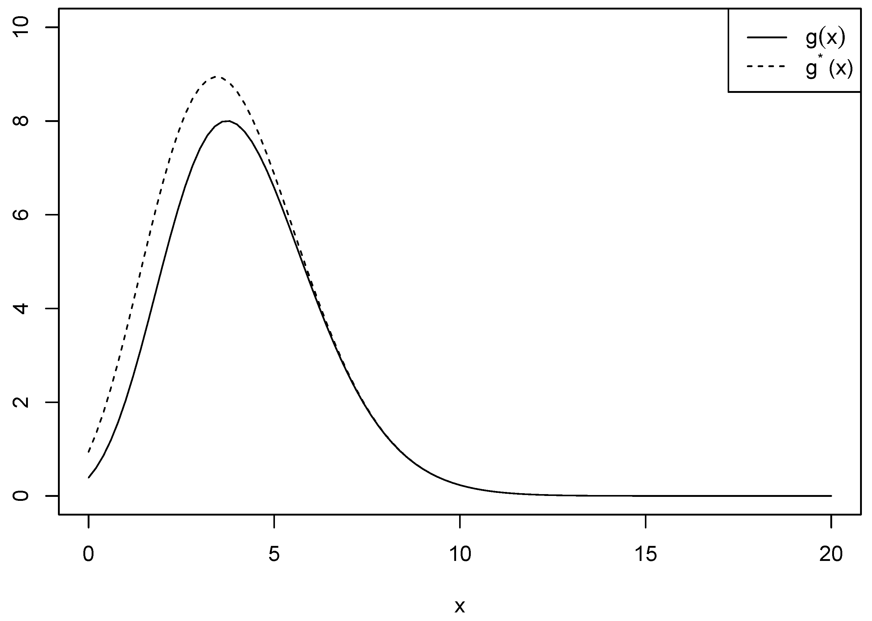
We provide some empirical calculations of the summand in (A1), which appears in the proof of Proposition 1 to justify the use of approximation. Let for simplicity, and let
be a function of x that should be manipulated through a reasonable approximation. Further, let
be another function used for approximation in which in is excluded. Figure 1 shows the two functions and when and for comparison purposes. We see that there is a number of differences between the ranges of the two functions for , while the difference vanishes when . We calculated the differences between and to ensure if the approximation is plausible. Table 1 provides the values of the differences when is and and is 3 and 4 for . We can see that the difference increases as increases, and it also increases as increases.
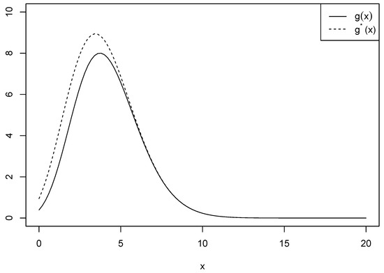
Figure 1.
Comparison of and when and .

Table 1.
The difference between and with different values of and .
3.3. Integral Prior
As mentioned in Section 2, Cano et al. [13] drew inspiration from the ideas of Peréz and Berger [22] to develop the concept of the integral prior. The proposed forms of the integral prior of each hypothesis are
and
Unlike Peréz and Berger [22], it can be observed that in (5) can be specified as distinct functions. Specifically, in (14) is obtained using the default prior, while the resulting is subsequently used to derive in (13).
Proposition 2.
The integral prior for under is
where k is a given constant and is called the zeta function, which is defined as
- The proof is provided in Appendix A.
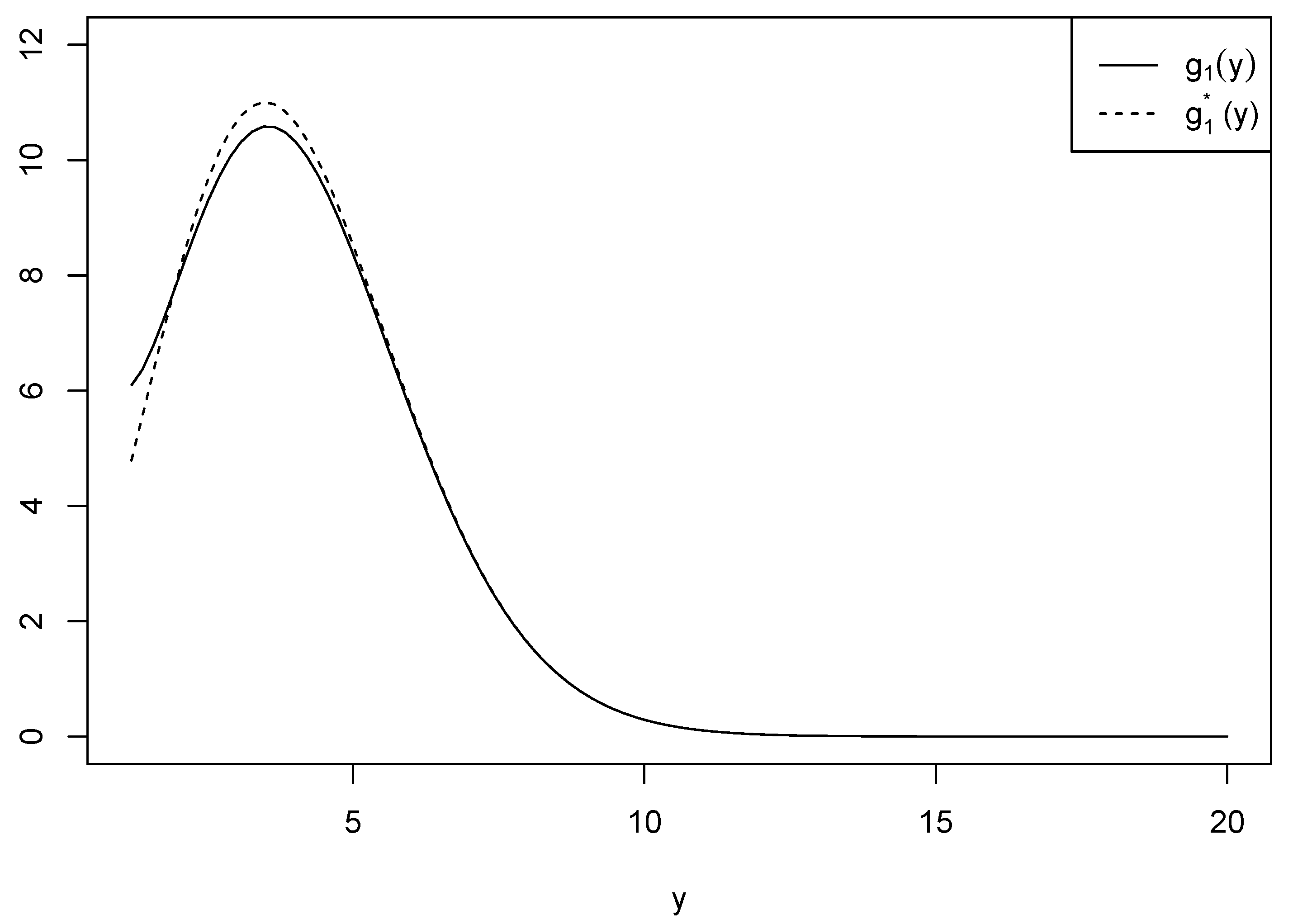
Similar to Proposition 1, an approximation method was utilized to obtain the result. For the purposes of consistency and simplicity in the analysis, we assumed . Let
be a function of y that should be manipulated through a reasonable approximation. Let
be another function used for approximation. Figure 2 shows the two functions and when for the comparison purposes conducted in Proposition 1.
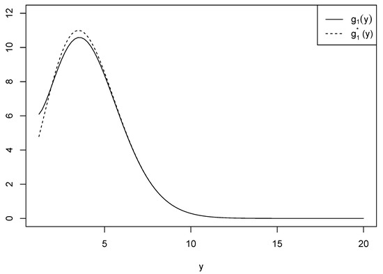
Figure 2.
Comparison of and when .
Proposition 3.
The integral prior for λ under is
where
Here k, , and are given constants, and is called a hypergeometric function and is defined as
Note that is called the rising factorial and is defined as .
- The proof is provided in Appendix A.
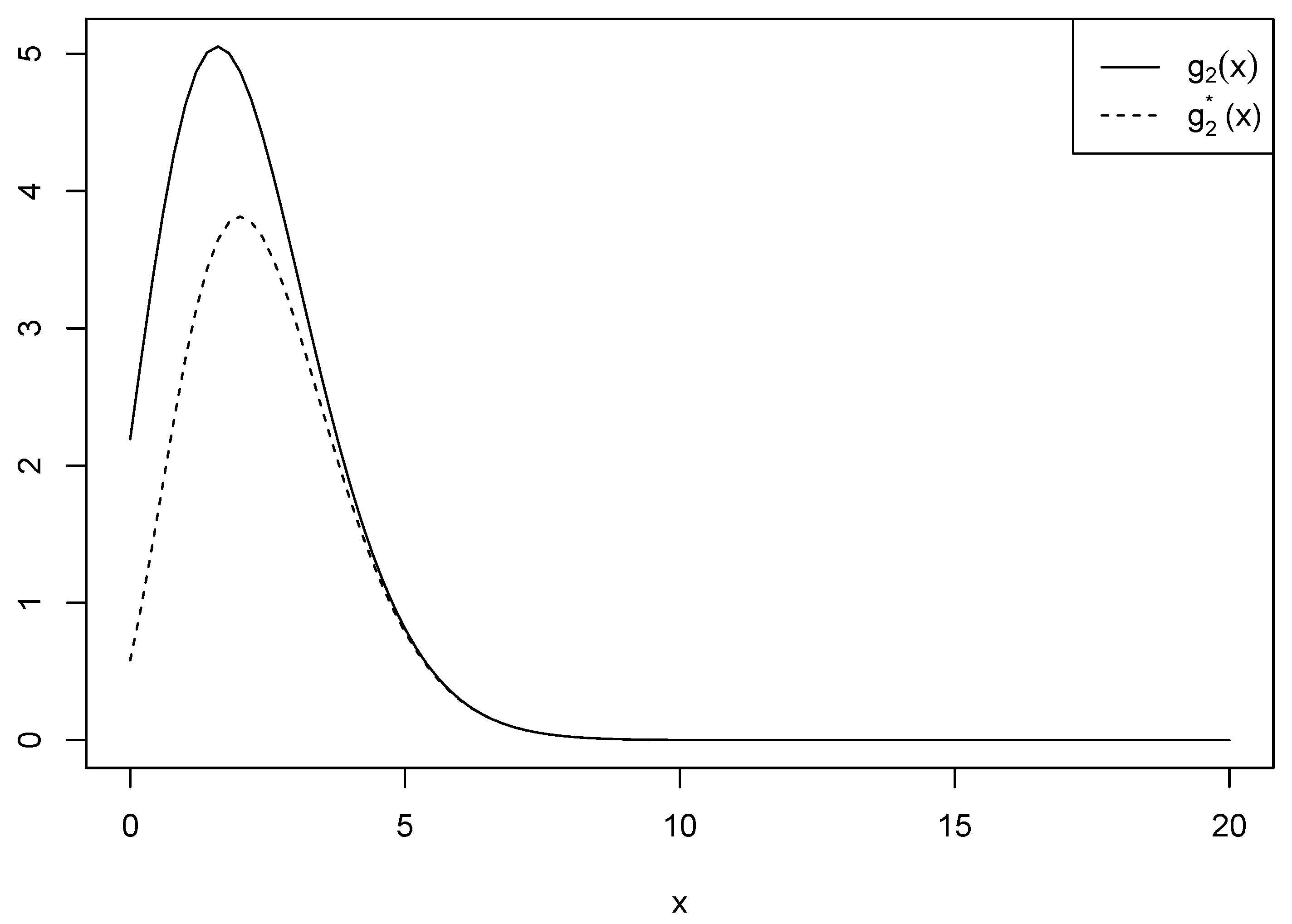
Two approximations are provided in the proof of Proposition 3. To proceed with the first approximation, let
be a function of x that should be manipulated through a reasonable approximation. Let
be another function used for approximation. Figure 3 shows the two functions and when and for comparison purposes. On the other hand, we noted that the second approximation closely resembled the approximation method used in Proposition 1.
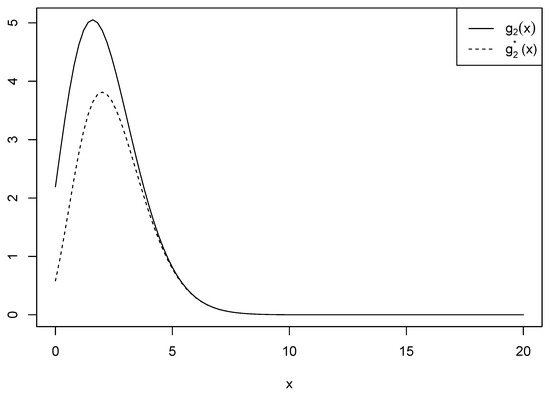
Figure 3.
Comparison of and when and .
We set to be associated with the intrinsic and integral priors in Propositions 1, 2, and 3 for both simulations and real data analyses.
3.4. An Encompassing Approach
Consider two nonnested hypotheses regarding based on a random sample from , that is, we are interested in testing
Since one cannot determine which model is more complex, Berger and Pericchi [10] suggested applying a global model, often called the encompassing model. Kim and Sun [24] conducted multiple tests on the power law process model using the encompassing approach. Sivaganesan and Jiang [17] used the encompassing model for testing the Poisson mean.
Let be the encompassing model. Then, the encompassing arithmetic Bayes factor of to is defined as
where is the Bayes factor of to based on the full Data with improper priors, and the correction factors are expressed as
and
where
Results for both simulations and real data analysis are presented in Section 4 and Section 5 to assess the model adequacy.
4. Simulation Studies
In this section, we conduct Monte Carlo simulations to evaluate the performance of default Bayes factors in testing the null hypothesis against the alternative when the underlying distribution follows a zero-inflated Poisson distribution with the parameters and . We generate data with four values of , and . We used two values of , 3 and 4, to identify an effect on . Regarding sample sizes, we used and 100 to check asymptotic behaviors. We calculated the default Bayes factor defined in (4) along with the two Bayes factors calculated with the intrinsic prior in (12) and the integral priors in (15) and (16), which are based only on the full sample and are denoted by and , respectively. We utilized R for our analysis, employing the parallel, doParallel, and foreach libraries for parallel processing. The pracma library was used to compute the Riemann zeta function, the hypergeo library for the hypergeometric function, and the cubature library for numerical integration.
Table 2 provides the simulated averages and standard deviations (in parentheses) of the three Bayes factors based on 1000 simulated data after eliminating 0.5% from both the top and bottom outliers. We also provide the median of the p-values based on the likelihood ratio test (LRT) to compare our Bayesian approach with the frequentist approach. Next, we provide four proportions based on 1000 replications: the proportion for which (supporting based on the Bayes factor), the proportion for which (supporting based on the LRT), the proportion for which both Bayesian and frequentist approaches support the true models (denoted by ), and the proportion for which both Bayesian and frequentist approaches have the same conclusions (denoted by ). First, we see that the direct approach works almost perfectly (in the sense that the two Bayes factors, and , are very close to each other on average). We noticed that there was a little discrepancy between and . Second, the results show that the proposed approach based on Bayes factors effectively identifies the true model, and the proportion supporting the true model increased as the sample size increased for most of the cases considered here. In particular, when the difference between and is 0.2, the Proportion increases rapidly as the sample size grows. This indicates that increasing sample sizes could entitle successful validations in which there is a not much difference between and . Regarding the comparison with the frequentist approach associated with the LRT, the proposed approach with Bayes factors provides comparable results in identifying the true model. Finally, there does not seem to be a large difference between and , though the results were slightly better when than when for all of the cases considered here.
Table 2.
The 0.5% trimmed average values and standard deviations (in parentheses) of the three Bayes factors based on 1000 replications. The following proportions are provided: , , , where both and the LRT support the true model; and : and the LRT yield the same conclusion.
Another simulation study was carried out for testing versus to assess the effectiveness of the encompassing approach presented in Section 3.4 by calculating the encompassing arithmetic Bayes factor defined in (17). We used three values (0.5, 0.6, and 0.7) to generate data by adding and subtracting 0.1 and 0.2 from . We also used the same values and sample sizes that were considered in the previous simulation setup. We report the posterior probability of defined in (1) instead of the Bayes factors so as to promptly check which of the two models identified the truth. Table 3 provides the results for the posterior probabilities with different configurations of parameters along with different sample sizes. Overall, the simulated data effectively support the true model. Specifically, the results are slightly better in terms of the posterior probabilities when is smaller. There did not appear to be large differences when changed.
Table 3.
Simulation results for testing versus based on the posterior probability. The results are based on 1000 replications.
5. Real Data Analysis
In this section, we demonstrate our proposed methodologies under the ZIP model with two real datasets possessing significant zero inflation patterns across time intervals. We calculated the default Bayes factors to see if they are close to each other. In addition, p-values based on the likelihood ratio test are reported for comparison purposes.
5.1. Yellow Dust Storm Data
We examined a dataset representing the number of yellow dust storms that occurred in South Korea during six-month intervals from the first half of 2003 to the second half of 2022. The sand and dust particles are mainly derived from the deserts in China and Mongolia, and they are carried by westerly winds from the Yangtze River, particularly in the spring season. Therefore, the frequency of yellow dust storms is dramatically higher during the first half of the year. We selected Incheon, a city in South Korea that is directly affected by yellow dust storms because it is only 360 km (about 224 miles) from mainland China. There are 10 zero observations from . Data are publicly accessible from the Korea Meteorological Administration website. Table 4 shows the results of testing with different values of that vary from 0.2 to 0.8 to see if the Bayes factors and the p-values effectively support the true models. We present the three Bayes factors along with the p-value as they were in the simulation study. The empirical proportion of zero observations is 25%, indicating that all three Bayes factors have minimum values at . Meanwhile, the p-value has a maximum value of 0.942 at , and decreases as moves away from 0.25.
Table 4.
Results of testing versus for yellow dust storm data. The three Bayes factors and p-values are provided with different values.
5.2. Book Reading Data
In this subsection, a reading dataset is employed to demonstrate the performance of the proposed methodologies as an illustration. The Korean Ministry of Culture, Sports, and Tourism has been conducting annual national reading surveys since 1993. The survey targets 6000 adults older than 19 years living in South Korea and asks the following: “How many paper books did you read from September 2020 to August 2021, excluding textbooks, reference books, and test preparation books?”. We extracted the data for male residents of Gyeonggi Province and gathered a total of 338 samples, 55.5% of which were zero observations. Table 5 shows the results for testing with a similar fashion to that which was conducted in Section 5.1. All three Bayes factors have minimum values at . On the other hand, the p-value has a maximum value of 0.959 at , as expected. Since we used a decently large sample of 338, a 5% differential from 0.55 yielded small p-values of 0.057 and 0.067 when is 0.5 and 0.6, respectively. These phenomena can also be observed for the Bayes factors.
Table 5.
Results of testing versus for book reading data. The three Bayes factors and the p-values are provided with different values.
6. Concluding Remarks
In this paper, we presented Bayesian testing procedures on the zero-inflated parameter in the zero-inflated Poisson distribution. We utilized a training sample to calculate the arithmetic intrinsic Bayes factor. Two types of priors were derived based on reasonable approximations. It turned out that the results were promising with the intrinsic prior outperforming the integral priors. We also tested nonnested hypotheses using the encompassing approach, and the simulation results showed that the true model was adequately captured. The proposed Bayesian approach and the existing frequentist approach with the likelihood ratio test were compared, and simulation studies yielded comparable results. Finally, two real datasets were analyzed to demonstrate practical applicability.
Since the Poisson distribution has the same mean and variance, discrepancies often arise as the actual data frequently exhibit different mean and variance values; this would be the most notable characteristic and limitation of the Poisson distribution. However, because of its inherent properties, the zero-inflated Poisson distribution naturally allows for a variance greater than the mean. Consequently, even when overdispersion occurs due to the presence of outliers in the data, the ZIP distribution can accommodate such variability to some extent.
There are some drawbacks in our approach that warrant further attention. While the three Bayes factors yielded similar values under the ZIP framework, the difference between the AIBF and the ordinary Bayes factor with the intrinsic prior should be expected to decrease in a consistent pattern as the sample size increases. However, this consistency is not perfectly observed. Analysis with extreme values or outliers is somewhat hindered due to overflow on numerical integration. Thus, there could be some limitations in calculations when the dataset contains these values. In addition, as appeared in the simulation studies, the results are better for larger values of . However, detailed explanations of these results are not available, necessitating further investigation. For future research, it is of our interest to consider a two-sample problem in testing both Poisson count parameter and the zero-inflated parameter in which default Bayesian procedures in conjunction with intrinsic and integral priors are proposed. Such research is in progress, and we hope to report the results in a future paper. Furthermore, it might be possible to find intrinsic and integral priors for the encompassing approach under our setup. This project may pose considerable challenges for future research.
Author Contributions
Conceptualization, J.H., K.K. and S.W.K.; methodology, J.H.; software, J.H.; validation, J.H., K.K. and S.W.K.; formal analysis, J.H.; investigation, J.H.; resources, J.H.; data curation, K.K.; writing—original draft preparation, J.H. and K.K.; writing—review and editing, J.H., K.K. and S.W.K.; visualization, J.H.; supervision, S.W.K.; project administration, S.W.K.; funding acquisition, K.K. and S.W.K. All authors have read and agreed to the published version of the manuscript.
Funding
K. Kim’s research was supported by the Basic Science Research Program through the National Research Foundation of Korea (NRF), which is funded by the Ministry of Education (NRF-202400000003334). S. W. Kim’s research was supported by the Basic Science Research Program through the National Research Foundation of Korea (NRF), which is funded by the Ministry of Education (NRF-2021R1A2C1005271).
Data Availability Statement
The original data presented in the study are openly available in the Korea Meteorological Administration at http://www.weather.go.kr and the Korean Ministry of Culture, Sports, and Tourism at https://mdis.kostat.go.kr/index.do.
Conflicts of Interest
The authors declare that they have no known competing financial interests or personal relationships that could have appeared to influence the work reported in this paper.
Appendix A
Proof of Proposition 1.
Note that follows a zero-truncated Poisson distribution with parameter . As such, we have
Now, let
Notice that in (A1) does not have a closed form due to the in the summand. We modified the summand to achieve a closed form through an approximation. Rewrite as
Thus, the result is readily obtained by the formula associated with the directional approach. □
Proof of Proposition 2.
Note that follows a zero-truncated Poisson distribution with parameter . As such, we have
□
Proof of Proposition 3.
To eliminate the nuisance parameter in , we integrated out with respect to . This results in having the following expression:
Thus, the marginal with becomes
Then, is calculated as follows:
Using the approximation process, the two infinite sums in become
and
Therefore, the integral prior for under is
□
References
- Cohen, A.C. Estimation in mixtures of two normal distributions. Technometrics 1967, 9, 15–28. [Google Scholar] [CrossRef]
- Lambert, D. Zero-inflated Poisson regression, with an application to defects in manufacturing. Technometrics 1992, 34, 1–14. [Google Scholar] [CrossRef]
- Hall, D.B. Zero-inflated Poisson and binomial regression with random effects: A case study. Biometrics 2000, 56, 1030–1039. [Google Scholar] [CrossRef] [PubMed]
- Yau, K.K.W.; Lee, A.H. Zero-inflated Poisson regression with random effects to evaluate an occupational injury prevention programme. Stat. Med. 2001, 20, 2907–2920. [Google Scholar] [CrossRef]
- Ghosh, S.K.; Mukhopadhyay, P.; Lu, J. Bayesian analysis of zero-inflated regression models. J. Stat. Plan. Inference 2006, 136, 1360–1375. [Google Scholar] [CrossRef]
- Yirdraw, B.S.; Debusho, L.K.; Samuel, A. Application of longitudinal multilevel zero inflated Poisson regression in modeling of infectious diseases among infants in Ethiopia. BMC Infect. Dis. 2024, 24, 927. [Google Scholar]
- Tshishimbi, W.M. Double robust semiparametric weighted M-estimators of a zero-inflated Poisson regression with missing data in covariates. Commun.-Stat.-Simul. Comput. 2024, 1–24. [Google Scholar] [CrossRef]
- Jeffreys, H. The Theory of Probability, 3rd ed.; Oxford University Press: New York, NY, USA, 1961; ISBN 978-01-9850-368-2. [Google Scholar]
- Berger, J.O.; Bernardo, J.M. Estimating a product of means: Bayesian analysis with reference priors. J. Am. Stat. Assoc. 1989, 84, 200–207. [Google Scholar] [CrossRef]
- Berger, J.O.; Pericchi, L.R. The intrinsic Bayes factor for model selection and prediction. J. Am. Stat. Assoc. 1996, 91, 109–122. [Google Scholar] [CrossRef]
- Lingham, R.T.; Sivaganesan, S. Intrinsic Bayes factor approach to a test for the power law process. J. Stat. Plan. Inference 1999, 77, 195–220. [Google Scholar] [CrossRef]
- Sanso, B.; Pericchi, L.R.; Moreno, E.; Racugno, W. On the robustness of the intrinsic Bayes factor for nested models [with discussion and rejoinder]. Lect. Notes-Monogr. Ser. 1996, 29, 155–173. [Google Scholar]
- Cano, J.A.; Robert, C.P.; Salmerón, D. Integral equation solutions as prior distributions for model selection. Test 2008, 17, 493–504. [Google Scholar] [CrossRef]
- Salmerón, D.; Cano, J.A.; Robert, C.P. Objective Bayesian hypothesis testing in binomial regression models with intgral prior distributions. Stat. Sin. 2015, 25, 1009–1023. [Google Scholar]
- Salmerón, D.; Cano, J.A.; Robert, C.P. On integral priors for multiple comparison in Bayesian model selection. arXiv 2024, arXiv:2406.14184. [Google Scholar]
- Bayarri, M.J.; García-Donato, G. Generalization of Jeffreys divergence-based priors for Bayesian hypothesis testing. J. R. Stat. Soc. Ser. B Stat. Methodol. 2008, 70, 981–1003. [Google Scholar] [CrossRef]
- Sivaganesan, S.; Jiang, D. Objective Bayesian testing of a Poisson mean. Commun. Stat.-Theory Methods 2010, 39, 1887–1897. [Google Scholar] [CrossRef]
- Han, Y.; Hwang, H.; Ng, H.K.T.; Kim, S.W. Default Bayesian testing for the zero-inflated Poisson distribution. Stat. Its Interface 2024, 17, 623–634. [Google Scholar] [CrossRef]
- Kass, R.E.; Raftery, A.E. Bayes factors. J. Am. Stat. Assoc. 1995, 90, 773–795. [Google Scholar] [CrossRef]
- Reid, N.; Mukerjee, R.; Fraser, D.A.S. Some aspects of matching priors. Lect. Notes-Monogr. Ser. 2003, 42, 31–43. [Google Scholar]
- Datta, G.S.; Mukerjee, R. Probability Matching Priors: Higher Order Asymptotics; Springer: New York, NY, USA, 2004; ISBN 978-0-387-20329-4. [Google Scholar]
- Peréz, J.M.; Berger, J.O. Expected-posterior prior distributions for model selection. Biometrika 2002, 89, 491–511. [Google Scholar] [CrossRef]
- Moreno, E.; Pericchi, L.R. Intrinsic priors for objective Bayesian model selection. Adv. Econom. 2014, 34, 279–300. [Google Scholar]
- Kim, S.W.; Sun, D. Intrinsic priors for model selection using an encompassing model with applications to censored failure time data. Lifetime Data Anal. 2000, 6, 251–269. [Google Scholar] [CrossRef]
Disclaimer/Publisher’s Note: The statements, opinions and data contained in all publications are solely those of the individual author(s) and contributor(s) and not of MDPI and/or the editor(s). MDPI and/or the editor(s) disclaim responsibility for any injury to people or property resulting from any ideas, methods, instructions or products referred to in the content. |
© 2025 by the authors. Licensee MDPI, Basel, Switzerland. This article is an open access article distributed under the terms and conditions of the Creative Commons Attribution (CC BY) license (https://creativecommons.org/licenses/by/4.0/).