Abstract
We consider time domain acoustic scattering from a bounded homogeneous penetrable obstacle. The problem is reduced to a system of time-dependent integral equations on the boundary of the scatter. Our aim is to determine the location and shape of the obstacle. Using convolution quadrature in time combined with the nonlinear integral equation method, we obtain the Helmholtz equation with complex wave numbers. Then the iterative scheme is presented to solve the nonlinear boundary integral equations, and the fully discrete system is given. Numerical experiments are presented to show the effectiveness of the proposed method.
Keywords:
inverse obstacle scattering; homogeneous penetrable obstacle; time domain; convolution quadrature; boundary integral equation MSC:
65N21
1. Introduction
Acoustic scattering problems have received increasing attention in diverse scientific areas such as medical diagnostics, ultrasound tomography, geophysical exploration, and nondestructive testing. However, compared with the frequency domain data, the time domain data is easier to get and contains more information at discrete frequencies. Thus, it is natural to consider the time domain inverse scattering problems. Although time domain inversion algorithms are more challenging due to the time dependence, different methods have been used to solve this problem either theoretically or numerically. Such as the enclosure method, linear sampling method, factorization method, Laguerre transform method, etc. For the framework of the enclosure method with dynamical data and its applications, we refer to [1]. For numerical examples of using the enclosure method for finding the convex hull of polygonal cavities, we refer to [2], and in the case of electromagnetic waves in the time domain, we refer to [3]. The advantage of this method is that one can calculate the support function of an unknown polygonal obstacle from only one measurement in a theoretical sense. However, the formula is ensured to work for estimating the value of the support function at only ‘regular’ directions. Using the enclosure method for the heat equation, we refer to [4], and for more details, we refer to [5,6]. The linear sampling method [7] is also a feasible tool in inverse acoustic scattering problems for the wave equation with Dirichlet, Robin, and Neumann boundary conditions from time domain measurements of scattered waves. In the article [8], the author determined the support of the inhomogeneity from measurements of causal scattered waves by using the linear sampling method in the time domain, and the first examples of using this method in three dimensions are included. The linear sampling method for sparse small aperture data we refer to [9]. Refer to [10,11,12,13,14,15] for more details of the linear sampling method. The factorization method [16] is used to characterize the Dirichlet scattering object from measurements of time-dependent causal scattered waves in the far field regime, and the method for obstacles with impedance boundary conditions in the time domain we refer to [17]. The Laguerre transform (LT) method is another useful tool for the acoustic scattering problem in the time domain. Compared with the Fourier–Laplace integral transform, the inverse transform of the LT method is to find the sum of corresponding Fourier–Laguerre series, which is proved to be more constructive. For more detail and applications of the LT method, we refer to [18,19,20].
In this paper, the inverse scattering problem we considered is the determination of the shape and location of an unknown homogeneous penetrable acoustic scatterer from the measurement of the scattered field in the time domain. Approaches based on retarded potentials are used since they reduce the time-dependent problem in the unbounded domain to an integral equation on the bounded surface. A particular class of methods for the discretization in time domain boundary integral equations (TDBIEs) for the wave equation are the so-called convolution quadratures (CQs); see Lunbich [21,22], in which Christian Lubich introduced this method by extending classical ideas of discrete operational calculus. This method is based on sustainable methods for ordinary differential equations and is more efficient than Galerkin or collocation time approximations. Refer to [23]; the author considered theoretically acoustic scattering problems with respect to various kinds of situations, such as scattering from sound soft, sound hard, non-penetrable, and penetrable with homogeneous or non-homogeneous media. For more details and applications of the CQ method, we refer to [24,25,26,27,28,29,30].
In this work, we propose the convolution quadrature method combined with the nonlinear integral equation method for the inverse problem. We note that this method is also used in [31] for the sound-soft obstacle. Specifically, the author uses the convolution quadrature method (CQ) for time discretization, and then a system of nonlinear integral equations-based iterative reconstruction method is developed to reconstruct both the location and shape of the obstacle. To our best knowledge, here the author first employs it in an inverse problem combined with a nonlinear integral equation method, which belongs to a simplified Newton method [32,33]. In this work, we also use the convolution quadrature method combined with the nonlinear integral equation method for the model of the homogeneous penetrable obstacle (see Equation (2) below). Given time-dependent scattering data, the Fourier transform of time-domain scattered field data is employed in the classic method, and then single frequency reconstruction methods are applied at several frequencies. Using the convolution quadrature method, we obtain a system of boundary integral equations for the Helmholtz equation with time-dependent complex wave numbers. Then, frequency-domain boundary integral operators are linearized with respect to the two-dimensional boundary’s parametrization to construct an iterative domain reconstruction method.
The outline of the paper is as follows. In Section 2, we formulate the direct and inverse scattering problem for the wave equation with a homogeneous penetrable obstacle. In Section 3, we obtain the boundary integral equations in the time domain and Laplace domain. In Section 4, we parameterize the curve and demonstrate that the regularized boundary integral equation has at least one solution in the frequency domain for the case of a ball-shaped obstacle. In Section 5, we introduce the convolution quadrature method for time discretization. In Section 6, an iterative scheme is presented, and the nonlinear boundary integral equation is linearized. Full discretization is given. In Section 7, numerical experiments are presented to demonstrate the effectiveness of the proposed methods. In Section 8, the conclusion of this paper with some future work. Detailed proof of eigenvalues of single-layer operator for unit circle is in Appendix A.
2. Problem Formulation
Let be a bounded open set in , and denote the complement of the scatter , with the common interface denoted by . Let denote the unit outward normal to . Given an incident wave field in free space, the scattering produced by the obstacle can be computed as follows [23]:
We assume the support of at time shall not intersect with the boundary of the obstacle . This assumption guarantees vanishing initial conditions for the scattered field and the total field inside the obstacle with their derivatives, respectively:
The physical parameters and are defined, respectively, by and , where is the density and c is the speed of propagation of sound. In this paper we only consider the situation where the obstacle is homogeneous and penetrable such that the parameters and are set to be constants. Thus, in the interior domain, the total field satisfies the equation:
Consequently, Equation (1) will be reduced to a system of equations as [23]
for which the incident wave satisfies
where the source term should not intersect with the obstacle.
The Inverse Problem. For a suitable constant , we define such that . Let the boundary be the observation curve. Using the incident wave emitted from a launch position and the scattered field received at observation curve , our aim is to locate the obstacle and predict the shape of it.
3. From Time Domain to Laplace Domain
The retarded single-layer potential with density in two dimensions is defined as follows [31]:
where
and H is the Heaviside function. The trace of a function u to the boundary from the interior and exterior of will be denoted and , respectively. The normal derivatives from inside and outside are and . Averages are denoted as follows [34]:
On the boundary, we define the following two operators:
The definitions above imply the jump relation of potentials [34]:
In this work, the scattered field and the interior total field in Equation (2) can be represented by a single layer potential as follows, with densities and , respectively.
Thus we have
From the boundary conditions and jump relations [34], we obtain the time domain boundary integral equations:
Now, we consider the corresponding Laplace-domain problem as follows:
and are the Laplace transforms of and , respectively, while is the Laplace transform of the income wave . We first recall the fundamental solution for the operator in two dimensions [34]:
where denotes the zero-order Hankel function of the first kind.
Consider the layer potential and integral operators associated with for . Given the density function , for arbitrary , the single layer potential has the expression in the frequency domain [34]:
Consequently, on the boundary, we can define two boundary integral operators [34]:
Using single layer potential for the problem (5), we assume that the exterior and interior solutions can be represented by
with densities and , respectively. Thus, on the boundary, we can define
and,
where is the Hankel function of the first kind of order one.
In the end, from the boundary conditions and jump relations [23], we obtain the Laplace domain boundary integral equations as follows:
4. Parameterization of the Curve
For brevity, let ; if correspondingly, . Now we can define new operators for some density :
We assume that the boundary is an analytic curve with the parametric form [35,36]
where is analytic and period with for all t. The normal derivative is represented by , while the outward unit normal derivative is denoted by . The parameterized integral operators are denoted by and , i.e.,
where
Firstly, we split the kernel into [36]
with
Accordingly,
Similarly, the kernel can be written in the form [36]
with analytic function
- where is known as Bessel function of order zero.
- Correspondingly,
Theorem 1.
The operators and are both compact operators from to .
Proof of Theorem 1.
Using (Theorem 12.15 [36]) and referring to [35], we can deduce that operators and are bounded from to for all . Consequently, both operators are compact from to .
Since the kernel functions and are analytic, it follows from (Theorem 8.13 [36]) and (Theorem A.45 [37]) that the operator and from to are bounded for all integers and arbitrary . Thus, we can deduce that the operator is compact from to .
Since the operator is bounded from to , the operator is also compact from to . □
Let ; assuming is not the eigenvalue of operator , then the operator has a bounded inverse . We can then turn the equation:
into the form
Let , . We can reformulate the above equation as
Since is a compact operator, Equation (11) is an integral equation of the first kind. For simplicity here, we only prove the existence of the solution of the regularized equation for the unit circle.
Let , and , and . We use the incident waves (40) to ensure that , both belong to for some ; thus, we have the following theorem:
Theorem 2.
For the trigonometric monomials , the eigenvalues of operator are tende to zero as . Let denote the linear subspace of generated by and denote the regularizer operator from to . Then, for Equation (11), there exists a solution satisfies the regularized equation: .
Remark 1.
Detailed proof of these eigenvalues; refer to Appendix A.
Proof of Theorem 2.
For , we first consider the series
It is easy to show that
where the series is absolutely convergent. Similarly, for the second and the third part of , the series
If we assume that , it is easy to compute that the series is absolutely convergent:
Similarly, for the second and third parts of , it is easy to show that the series
and
satisfy the inequality (assuming , ; , ):
for some constant . It is clear that the series and are both absolutely convergent. Accordingly, tends to zero, as . □
With the eigenfunctions , the eigenvalues are as follows:
for ,
- Here, we define , , denote Euler’s constant.
- For ,
- are both absolutely convergent.
- For we consider the second part of :
5. Time Discretization
We use the convolution quadrature method [29,31] to handle the time discretization of the boundary integral Equation (4). Briefly, the right-hand side of expression (3) can be written as
where w is a parameter-dependent integral operator:
The Laplace transform of w is defined by
Its specific expression has the form
where .
In order to discretize the time convolution, we split the time interval into time steps of equal length with ,. Then, using the convolution quadrature method [29,31], we replace the continuous convolution operator at the discrete times by the discrete convolution operator, for ,
The convolution weights are defined below:
where is the quotient of the generating polynomials of the BDF2 scheme. As recommended in [31], the convolution weights have their representation as a contour integral
where C can be chosen as a circle centered at the origin of radius . Using the trapezoidal rule, the approximate convolution weights are given by
where , . Substituting the definition of in (15), we obtain the expression as follows:
where
Using the above results, for the time domain boundary integral to Equation (4), we can define new discrete convolution quadrature operators as follows:
The time-discrete problem is given as follows: find , such that
where and are some approximations to and , respectively. For the above Equation (22), applying the discrete Fourier transform to both sides, we finally get the following decoupled boundary integral equations
where and are the scaled discrete Fourier transform
Similarly, and are the scaled discrete Fourier transform
Ultimately, we obtain the densities and by applying the inverse transform
Because the scaled discrete Fourier transform of has the expression
for , , the scattering wave is given by
6. The Inverse Scheme
6.1. Nonlinear Integral Equations
For brevity, we use the symbols as follows:
and
where and
Then, we can get the parameterized expressions of Equation (23) as
- where
- For simplicity, we use symbols to represent the retarded single layer potential (3)
6.2. Fully Discretization
Next, we describe the full discretization of (29) and (36). Let , be equidistant sets of quadrature knots. Seting , and , for and . Using the Nystrom method [36], we can get the full discretization of (29)
for , , where
Meanwhile, we can decuce the diagonal term as
with the Euler constant . Similarly,
and the diagonal term is
Next, we discretize the linearized Equation (36) to obtain the update by using least squares with Tikhonov regularization [37,38]. We choose the space of trigonometric polynomials of the form [31] to approximate the radial function r and its update
where the integer is the truncation number. We can reformulate Equation (36) as follows; for details of the fully discretization, we refer to [31].
Utilizing the trapezoidal rule, we obtain the discretized linear system from (33)–(36)
to determine the real coefficients , and , where
and
Since , due to the ill-posedness, the Tikhonov regularization can be used to tackle the overdetermined system (37). Thus, the linear system (37) is turned into the following function [31,38]:
with a positive regularization parameter and penalty term. It is clear that the minimizer of above equation is the solution of the system
where
Consequently, the new approximation is obtained
7. Numerical Experiments
For the numerical experiments, we considered the following income wave, defined by
which is emitted from a single launch position such that the incident wave clearly satisfies the two-dimensional time-domain wave equation. The scattered field data are numerically computed at 60 points, .e., . And 100 quadrature nodes are chosen for the direct problem and 64 quadrature nodes for the inverse problem. We construct the noisy data in the following way [38]: , where are random numbers ranging in , is the relative noise level. By using the Tikhonov regularization and penalty term, we will get the update from a scaled Newton step, i.e.,
where the scaling factor is a fixed number throughout the iteration. Analogously to [31], the regularization parameters in (39) are chosen as
Analogously to [31,38], we choose the update when the norm of the right hand is less than the tolerance: .
Numerical Examples. Inverse acoustic scattering problem for a homogeneous penetrable obstacle with a single launch position. We investigate the inverse scattering problem of reconstructing a homogeneous penetrable obstacle from the scattered-field data in the time domain, including the shape and the position. The reconstructions with different noise levels for the acorn-shaped, bean-shaped, peanut-shaped, and kite-shaped obstacles are shown in Figure 1, Figure 2, Figure 3, and Figure 4, respectively. The numerical results show that the reconstruction of a homogeneous penetrable obstacle deals with the angle of the incident wave, the position and radius of the initial guess, the shape of the obstacle, and the size of the noise level. These results show that the reconstruction is not sensitive to the initial guess or the launch position of the incident wave, although there will be a large error in reconstructing the shape of the obstacle at some cusp positions, and the error is within our control. Note that all the programs are written using Matlab.
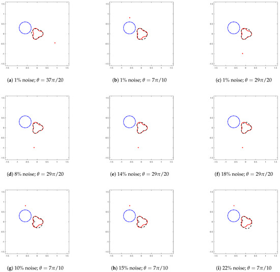
Figure 1.
Reconstruction of an acorn-shaped obstacle at different levels of noise. The radius of the initial guess is . The position of the initial guess is . The (a–c) show that when we keep the initial guess unchanged and incident waves from different angles, we can have a better reconstruction effect, except that the error of the reconstruction far away from the point source is a little large. But the result is in line with our expectations. The results of (d–i) show that when we increase the noise level, the reconstruction method is still used, but the error will be larger.
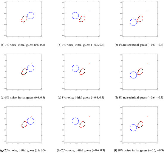
Figure 2.
Reconstruction of a bean-shaped obstacle at different levels of noise. The angle of incident wave is . We keep the angle of the incident wave unchanged while the initial guess is in different position. (a–c) show that for bean-shaped obstacles, the change in initial guess position does not affect the effectiveness of the reconstruction method, except that the error of the reconstruction far away from the point source is a little large, such as (f) shows. (d–i) shows that when we increase the noise level, the reconstruction method still works. But compared with the reconstruction results of acorn-shaped obstacles, it (i) tells us that even if we enhance the noise level to , the method still performs well (But when we enhance the noise level to , the error is too large to accept).
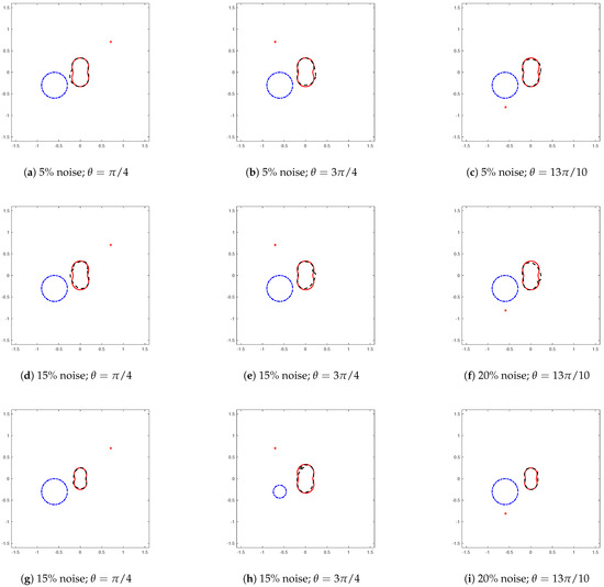
Figure 3.
Reconstruction of a peanut-shaped obstacle at different levels of noise. The position of the initial guess is . In (h), the radius of initial guess is , while the others are . (a–c) show that for peanut-shaped obstacle, when we fixed the initial guess, the reconstruction method is effective for incident waves at different angles. (d–i) show that when we increase the noise level, the reconstruction method still works. However, by comparing (d,g), we find that after fixing the incident wave angle and noise level, adjusting the relative size of the initial guess and the obstacle has an impact on the accuracy of the reconstruction results. As the result of (g) shows, when we reduce the size of the obstacle, the reconstruction result is better than that of (d). We can get same results from (e,f,h,i).
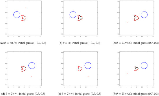
Figure 4.
Reconstruction of a kite-shaped obstacle. The noise level is , and the radius of initial guess is . (a–f) shows that even if we keep the noise level at for the reconstruction of kite-shaped obstacle, the angle of the incident wave will have a relatively large impact on the reconstruction results. The (d) clearly shows that. But this is also in line with our expectations. Further, as the results of (d–f) show, when we reduce the size of the obstacle, the reconstruction result is better. Note that the parametric equations for kite-shaped obstacle are set to be ; In (d,e), we choose r to be and , respectively, while in (f), r is set to be .
In all the following figures, the exact boundary curves are expressed by solid lines while the reconstructed boundary curves are displayed by dashed lines , and all the initial guesses are taken to be a circle with radius , which is indicated by the dash-dotted lines . The position of incident waves is marked by an asterisk *. We choose , the radius of the observation curve , the center of the observation curve , the scaling factor , the cycle index for per , and the truncation .
8. Conclusions
In this paper, we have studied the two-dimensional inverse acoustic scattering from a homogeneous penetrable obstacle. The challenge of the time domain inverse problem is due to the time dependence. The fact that we obtain a convolution equation suggests the possibility of using CQ methods for the time variable. Although we obtain expressions for the time-domain potentials, we will write all the equations in the frequency domain. However, it has to be understood that this method works in the time domain, and the solutions are computed in a time-stepping fashion. The fact that we use the operators in the frequency domain (which is a requisite of CQ) does not mean that we are going to solve at that domain and then invert the Laplace transform.
That scattered waves outside the obstacle and the total wave inside the obstacle are both represented by a single-layer potential, resulting in the boundary integral equation reformulating to an integral equation of the first kind. Thus, we only prove the existence of the solution of the boundary integral equation under regularization. But this is not conducive to accurate numerical analysis. This is one of the problems that we will solve in our follow-up work. A nonlinear integral equation method is developed for the inverse problem, and numerical examples are presented to demonstrate the effectiveness and stability of the method. In summary, the angle of the incident wave, the position and radius of the initial guess, the shape of the obstacle, and the size of the noise level all affect the reconstruction results. All the numerical experiment results show the method presented in this paper is very effective for retrieving the position of the obstacle, and there will be a large error in reconstructing the shape of the obstacle at some cusp positions, which is also related to the angle of the incident wave. For example, the results of reconstruction for kite-shaped obstacles do not perform as well as for bean-shaped obstacles. From the results of numerical experiments, we can also see that for a bean-shaped obstacle, even if we enhance the noise level to , the method still works, while for a kite-shaped obstacle, the results are barely acceptable for a noise level. Similar results can be found in the literature [31], which uses the same method to reconstruct the position and shape of sound soft obstacles. In general, these results show that the reconstruction is not sensitive to the initial guess or the launch position of the incident wave. Future work includes the application to other inverse acoustic scattering problems for non-homogeneous penetrable obstacles and error analysis.
Author Contributions
Writing—original draft, Z.Q.; Writing—review & editing, F.M. All authors have read and agreed to the published version of the manuscript.
Funding
This research received no external funding.
Data Availability Statement
The original contributions presented in this study are included in the article. Further inquiries can be directed to the corresponding author.
Conflicts of Interest
The authors declare no conflicts of interest.
Appendix A
The main content of the appendix is how to calculate the eigenvalue of the single-layer operator in the case of the unit circle. Retrospective the Formula (8), its specific expression is:
The main procedure is to divide the above operator into three parts to calculate. After a simple substitution, our aim is to calculate Equations (A3) and (A12). We solve (A3) by calculating (A4) and (A5). Solve (A13) to get the result of (A12). The main calculation skills see Problem A1 and Problem A2.
We consider the first part of Equation (A1):
We substitute for ; then, we have
First we focus on the integral
We use the integral followed to tackle Equation (A3):
Refer to Problem A1, we have
Similarly,
Refer to Problem A1, we have
From (A2)–(A8), we conclude that
For the second part of Equation (A1), we substitute for , then the Equation (A1) turns into
We first consider the expression
By simple calculation, we obtain
and we utilize the contour integral
to handle the right side of the expression (A12), where C denote the unit circle and is a possible singularity. Let ,
Using the Residue theorem, we have
for detailed proof we refer to Problem A2. Then, we can write that
For the second part of (A1), we consider the expression
It is easy to show that
And for simple computation, we have
From (A15), we will have
Problem A1.
Compute the integral: .
Proof.
and
Thus, the integral in the upper semicircle
and the integral in the lower semicircle
Next,
and
Thus we can write that
Next, we compute
For easy computation, we obtain
thus,
We can conclude that, for and ,
Secondly, we compute
For , then is always a singularity. Let , then is a pole of it with order . Let ,
For and , we have
Next for ,
And
Finally, we have
We utilize contour integral
- to resolve the problem. C denote the integral curve, which is unite circle and from [39,40], we have with denote a half circle and its radius is .

- Let , for , we have
(1) if and , then is a removable singularity of ; thus, the integral is equal to zero.
(2) if and , then is a pole of
- with order . Let
- Then, we have
□
Problem A2.
Compute the integral:
Proof.
(1) if and , is removable singularity; thus, the integral is equal to zero.
- (2) if and , is a pole of order .
- Let , then we havethus,(3) if and , the integral is equal to zero. and for , the integral is equal to . □
References
- Ikehata, M. The framework of the enclosure method with dynamical data and its applications. Inverse Probl. 2011, 27, 065005. [Google Scholar] [CrossRef]
- Ikehata, M.; Ohe, T. A numerical method for finding the convex hull of polygonal cavities using the enclosure method. Inverse Probl. 2002, 18, 111. [Google Scholar] [CrossRef]
- Ikehata, M. The enclosure method for inverse obstacle scattering using a single electromagnetic wave in time domain. arXiv 2013, arXiv:1401.0083. [Google Scholar] [CrossRef]
- Ikehata, M.; Kawashita, M. The enclosure method for the heat equation. Inverse Probl. 2009, 25, 075005. [Google Scholar] [CrossRef]
- Ikehata, M. The enclosure method for inverse obstacle scattering problems with dynamical data over a finite time interval. Inverse Probl. 2010, 26, 055010. [Google Scholar] [CrossRef]
- Ikehata, M. Revisiting the probe and enclosure methods. Inverse Probl. 2022, 38, 075009. [Google Scholar] [CrossRef]
- Haddar, H.; Lechleiter, A.; Marmorat, S. An improved time domain linear sampling method for Robin and Neumann obstacles. Appl. Anal. 2014, 93, 369–390. [Google Scholar] [CrossRef][Green Version]
- Guo, Y.; Monk, P.; Colton, D. Toward a time domain approach to the linear sampling method. Inverse Probl. 2013, 29, 095016. [Google Scholar] [CrossRef]
- Guo, Y.; Monk, P.; Colton, D. The linear sampling method for sparse small aperture data. Appl. Anal. 2016, 95, 1599–1615. [Google Scholar] [CrossRef]
- Cakoni, F.; Colton, D. On the mathematical basis of the linear sampling method. Georgian Math. J. 2003, 411–425. [Google Scholar] [CrossRef]
- Arens, T.; Lechleiter, A. The linear sampling method revisited. J. Integral Equ. Appl. 2009, 21, 179–202. [Google Scholar] [CrossRef]
- Arens, T. Why linear sampling works. Inverse Probl. 2003, 20, 163. [Google Scholar] [CrossRef]
- Cakoni, F.; Colton, D. The linear sampling method for cracks. Inverse Probl. 2003, 19, 279. [Google Scholar] [CrossRef]
- Chen, Q.; Haddar, H.; Lechleiter, A.; Monk, P. A sampling method for inverse scattering in the time domain. Inverse Probl. 2010, 26, 085001. [Google Scholar] [CrossRef]
- Cakoni, F.; Monk, P.; Selgas, V. Analysis of the linear sampling method for imaging penetrable obstacles in the time domain. Anal. PDE 2021, 14, 667–688. [Google Scholar] [CrossRef]
- Cakoni, F.; Haddar, H.; Lechleiter, A. On the factorization method for a far field inverse scattering problem in the time domain. SIAM J. Math. Anal. 2019, 51, 854–872. [Google Scholar] [CrossRef]
- Haddar, H.; Liu, X. A time domain factorization method for obstacles with impedance boundary conditions. Inverse Probl. 2020, 36, 105011. [Google Scholar] [CrossRef]
- Litynskyy, S.; Muzychuk, Y.; Muzychuk, A. On the numerical solution of the initial-boundary value problem with neumann condition for the wave equation by the use of the laguerre transform and boundary elements method. Acta Mech. Autom. 2016, 10, 285–290. [Google Scholar] [CrossRef]
- Hlova, A.; Litynskyy, S.; Muzychuk Yu, A.; Muzychuk, A. Coupling of Laguerre transform and Fast BEM for solving Dirichlet initial-boundary value problems for the wave equation. J. Comput. Appl. Math 2018, 128, 42–60. [Google Scholar]
- Litynskyy, S.; Muzychuk, A. Solving of initial-boundary value problems for the wave equation using retarded surface potential and Laguerre transform. Mat. Stud. 2015, 44, 185–203. [Google Scholar] [CrossRef]
- Lubich, C. Convolution quadrature and discretized operational calculus. I. Numer. Math. 1988, 52, 129–145. [Google Scholar] [CrossRef]
- Lubich, C. Convolution quadrature and discretized operational calculus. II. Numer. Math. 1988, 52, 413–425. [Google Scholar] [CrossRef]
- Laliena, A.R.; Sayas, F.J. Theoretical aspects of the application of convolution quadrature to scattering of acoustic waves. Numer. Math. 2009, 112, 637–678. [Google Scholar] [CrossRef]
- Lubich, C. Convolution quadrature revisited. BIT Numer. Math. 2004, 44, 503–514. [Google Scholar] [CrossRef]
- Labarca, I.; Hiptmair, R. Acoustic scattering problems with convolution quadrature and the method of fundamental solutions. Commun. Comput. Phys. 2021, 30, 985–1008. [Google Scholar] [CrossRef]
- Aldahham, E.; Banjai, L. A modified convolution quadrature combined with the method of fundamental solutions and Galerkin BEM for acoustic scattering. arXiv 2022, arXiv:2203.00996. [Google Scholar]
- Ballani, J.; Banjai, L.; Sauter, S.A.; Veit, A. Numerical solution of exterior Maxwell problems by Galerkin BEM and Runge-Kutta convolution quadrature. Numer. Math. 2013, 123, 643–670. [Google Scholar] [CrossRef]
- Lubich, C. On the multistep time discretization of linear initial-boundary value problems and their boundary integral equations. Numer. Math. 1994, 67, 365–389. [Google Scholar] [CrossRef]
- Banjai, L.; Sauter, S. Rapid solution of the wave equation in unbounded domains. SIAM J. Numer. Anal. 2009, 47, 227–249. [Google Scholar] [CrossRef]
- Banjai, L.; Lubich, C. An error analysis of Runge–Kutta convolution quadrature. BIT Numer. Math. 2011, 51, 483–496. [Google Scholar] [CrossRef]
- Zhao, L.; Dong, H.; Ma, F. Inverse obstacle scattering for acoustic waves in the time domain. Inverse Probl. Imaging 2021, 15, 1269. [Google Scholar] [CrossRef]
- Ivanyshyn, O.; Johansson, T. Nonlinear integral equation methods for the reconstruction of an acoustically sound-soft obstacle. J. Integral Equ. Appl. 2007, 19, 289–308. [Google Scholar] [CrossRef]
- Johansson, T.; Sleeman, B.D. Reconstruction of an acoustically sound-soft obstacle from one incident field and the far-field pattern. IMA J. Appl. Math. 2007, 72, 96–112. [Google Scholar] [CrossRef]
- Sayas, F.J. Retarded Potentials and Time Domain Boundary Integral Equations: A Road Map; Springer: Berlin/Heidelberg, Germany, 2016; Volume 50. [Google Scholar]
- Dong, H.; Lai, J.; Li, P. A highly accurate boundary integral method for the elastic obstacle scattering problem. Math. Comput. 2021, 90, 2785–2814. [Google Scholar] [CrossRef]
- Kress, R. Linear Integral Equations; Springer: Berlin/Heidelberg, Germany, 1989. [Google Scholar]
- Kirsch, A. An Introduction to the Mathematical Theory of Inverse Problems; Springer: Berlin/Heidelberg, Germany, 2011; Volume 120. [Google Scholar]
- Dong, H.; Zhang, D.; Guo, Y. A reference ball based iterative algorithm for imaging acoustic obstacle from phaseless far-field data. arXiv 2018, arXiv:1804.05062. [Google Scholar] [CrossRef]
- Courant, R.; Hilbert, D. Methoden der Mathematischen Physik; Springer: Berlin/Heidelberg, Germany, 2013. [Google Scholar]
- Dennery, P.; Krzywicki, A. Mathematics for Physicists; Courier Corporation: Chelmsford, MA, USA, 2012. [Google Scholar]


Disclaimer/Publisher’s Note: The statements, opinions and data contained in all publications are solely those of the individual author(s) and contributor(s) and not of MDPI and/or the editor(s). MDPI and/or the editor(s) disclaim responsibility for any injury to people or property resulting from any ideas, methods, instructions or products referred to in the content. |
© 2025 by the authors. Licensee MDPI, Basel, Switzerland. This article is an open access article distributed under the terms and conditions of the Creative Commons Attribution (CC BY) license (https://creativecommons.org/licenses/by/4.0/).