A Non-Self-Referential Characterization of the Gram–Schmidt Process via Computational Induction

Abstract

The Gram–Schmidt process (GSP) plays an important role in algebra. It provides a theoretical and practical approach for generating an orthonormal basis, QR decomposition, unitary matrices, etc. It also facilitates some applications in the fields of communication, machine learning, feature extraction, etc. The typical GSP is self-referential, while the non-self-referential GSP is based on the Gram determinant, which has exponential complexity. The motivation for this article is to find a way that could convert a set of linearly independent vectors ${\left\{{\overrightarrow{u}}_i\right\}}_{j=1}^n$ into a set of orthogonal vectors ${\left\{\overrightarrow{v}\right\}}_{j=1}^n$ via a non-self-referential GSP (NsrGSP). The approach we use is to derive a method that utilizes the recursive property of the standard GSP to retrieve a NsrGSP. The individual orthogonal vector form we obtain is ${\displaystyle {\overrightarrow{v}}_k=\sum _{j=1}^k{\beta }_{[k\to j]}{\overrightarrow{u}}_j}$, and the collective orthogonal vectors, in a matrix form, are $V_k=U_k\left(B_{{\Delta }_k}^{+}\right)$. This approach could reduce the exponential computational complexity to a polynomial one. It also has a neat representation. To this end, we also apply our approach on a classification problem based on real data. Our method shows the experimental results are much more persuasive than other familiar methods.

1. Introduction

The Gram–Schmidt method plays an important role in both theoretical and practical aspects. It has also been applied in constructing some orthogonal elements in some algebraic systems [1], in signal processing [2], and in QR decomposition [3,4] (although there are other approaches to the QR problem [5]). In addition, it could also be applied to machine learning and feature extraction [6,7] via a modified Gram–Schmidt method [8]. However, one would like to have a non-self-referential form of the GSP; but the typical one is in a formal determinant form—whose computational complexity is exponentially high and whose form is not succinctly presented. There is a research gap in bridging the typical (self-referential) and the non-self-referential GSP. This motivates our research on finding a non-self-referential method that could reduce the complexity and enhance the presentation. The novelty part of this article is to find the internal recursive relation between the input vectors U and the converted orthogonal vectors V, as well as a hypothesis of the non-self-referential form and a proof that our hypothesis is correct. Let $\mathbb{R}$ denote the set of real numbers. Let $(W,•)$ denote an inner product space, where the inner product $•:W\times W\to \mathbb{R}$ satisfies $\overrightarrow{u}•\overrightarrow{v}=\overrightarrow{v}•\overrightarrow{u}$, $\overrightarrow{u}•\overrightarrow{u}\ge 0$, $\overrightarrow{u}•\overrightarrow{u}=0\Rightarrow \overrightarrow{u}=0\in W$, and $(\alpha \overrightarrow{u}+\beta \overrightarrow{v})•\overrightarrow{w}=\alpha ·(\overrightarrow{u}•\overrightarrow{w})+\beta ·(\overrightarrow{v}•\overrightarrow{w})$ for all $\alpha ,\beta \in \mathbb{R}$ and all $\overrightarrow{u},\overrightarrow{v},\overrightarrow{w}\in W$. Let $U=\{{\overrightarrow{u}}_1,{\overrightarrow{u}}_2,\cdots ,{\overrightarrow{u}}_m\}\subseteq W$ be a set of independent vectors, i.e., U is a basis. Then, one associates by the Gram–Schmidt method, the following:

• ${\overrightarrow{v}}_1={\overrightarrow{u}}_1;{\overrightarrow{\omega }}_1={\displaystyle \frac{{\overrightarrow{v}}_1}{\left|\right|{\overrightarrow{v}}_1\left|\right|}}$;
• ${\overrightarrow{v}}_2={\overrightarrow{u}}_2-({\overrightarrow{u}}_2•{\overrightarrow{w}}_1){\overrightarrow{w}}_1;{\overrightarrow{w}}_2={\displaystyle \frac{{\overrightarrow{v}}_2}{\left|\right|{\overrightarrow{v}}_2\left|\right|}}$;
• ${\overrightarrow{v}}_3={\overrightarrow{u}}_3-({\overrightarrow{u}}_3•{\overrightarrow{w}}_1){\overrightarrow{w}}_1-({\overrightarrow{u}}_3•{\overrightarrow{w}}_2){\overrightarrow{w}}_2;{\overrightarrow{w}}_3={\displaystyle \frac{{\overrightarrow{v}}_3}{\left|\right|{\overrightarrow{v}}_3\left|\right|}}$;
  ⋮
• ${\displaystyle {\overrightarrow{v}}_k={\overrightarrow{u}}_k-\sum _{i=1}^{k-1}({\overrightarrow{u}}_k•{\overrightarrow{w}}_i){\overrightarrow{w}}_i;{\overrightarrow{w}}_k=\frac{{\overrightarrow{v}}_k}{\left|\right|{\overrightarrow{v}}_k\left|\right|}}$;
• ${\displaystyle {\overrightarrow{v}}_{k+1}={\overrightarrow{u}}_{k+1}-\sum _{i=1}^k({\overrightarrow{u}}_{k+1}•{\overrightarrow{w}}_i){\overrightarrow{w}}_i;{\overrightarrow{w}}_{k+1}=\frac{{\overrightarrow{v}}_{k+1}}{\left|\right|{\overrightarrow{v}}_{k+1}\left|\right|}}$;
  ⋮
• ${\displaystyle {\overrightarrow{v}}_m={\overrightarrow{u}}_m-\sum _{j=1}^{m-1}({\overrightarrow{u}}_m•{\overrightarrow{w}}_j){\overrightarrow{w}}_j;{\overrightarrow{w}}_m=\frac{{\overrightarrow{v}}_m}{\left|\right|{\overrightarrow{v}}_m\left|\right|}}$.

This can also be represented in a matrix form: $\left[\begin{array}{c}{\overrightarrow{v}}_1\\ {\overrightarrow{v}}_2\\ {\overrightarrow{v}}_3\\ ⋮\\ {\overrightarrow{v}}_{k+1}\\ ⋮\\ {\overrightarrow{v}}_m\end{array}\right]=\left[\begin{array}{c}{\overrightarrow{u}}_1\\ {\overrightarrow{u}}_2\\ {\overrightarrow{u}}_3\\ ⋮\\ {\overrightarrow{u}}_{k+1}\\ ⋮\\ {\overrightarrow{u}}_m\end{array}\right]-\left[\begin{array}{ccccccc}0& 0& 0& \cdots & 0& \cdots & 0\\ 0& {\overrightarrow{u}}_2•{\overrightarrow{w}}_1& 0& \cdots & 0& \cdots & 0\\ 0& {\overrightarrow{u}}_3•{\overrightarrow{w}}_1& {\overrightarrow{u}}_3•{\overrightarrow{w}}_2& \cdots & 0& \cdots & 0\\ ⋮\\ 0& {\overrightarrow{u}}_{k+1}•{\overrightarrow{w}}_1& {\overrightarrow{u}}_{k+1}•{\overrightarrow{w}}_2& \cdots & {\overrightarrow{u}}_{k+1}•{\overrightarrow{w}}_k& \cdots & 0\\ ⋮\\ 0& {\overrightarrow{u}}_m•{\overrightarrow{w}}_1& {\overrightarrow{u}}_m•{\overrightarrow{w}}_2& \cdots & {\overrightarrow{u}}_m•{\overrightarrow{w}}_k& \cdots & {\overrightarrow{u}}_m•{\overrightarrow{w}}_{m-1}\end{array}\right]\left[\begin{array}{c}1\\ {\overrightarrow{w}}_1\\ {\overrightarrow{w}}_2\\ ⋮\\ {\overrightarrow{w}}_k\\ ⋮\\ {\overrightarrow{w}}_{m-1}\end{array}\right]$ This is a typical self-referential (or where ${\overrightarrow{v}}_k$ is explicitly dependent on ${\left\{{\overrightarrow{v}}_j\right\}}_{j=1}^{k-1}$) version of the Gram–Schmidt process (GSP). For the non-self-referential version of the Gram–Schmidt process (see [9], Chapter 7), one often resorts to the Gram determinant in the following formula:

$${\overrightarrow{v}}_k=FDET(\left[\begin{array}{cccc}{\overrightarrow{u}}_1•{\overrightarrow{u}}_1& {\overrightarrow{u}}_1•{\overrightarrow{u}}_2& \cdots & {\overrightarrow{u}}_1•{\overrightarrow{u}}_k\\ {\overrightarrow{u}}_2•{\overrightarrow{u}}_1& {\overrightarrow{u}}_2•{\overrightarrow{u}}_2& \cdots & {\overrightarrow{u}}_2•{\overrightarrow{u}}_k\\ ⋮& ⋮& \cdots & ⋮\\ {\overrightarrow{u}}_{k-1}•{\overrightarrow{u}}_1& {\overrightarrow{u}}_{k-1}•{\overrightarrow{u}}_2& \cdots & {\overrightarrow{u}}_{k-1}•{\overrightarrow{u}}_k\\ {\overrightarrow{u}}_1& {\overrightarrow{u}}_2& \cdots & {\overrightarrow{u}}_k\end{array}\right]),$$

(1)

where $FDET$ stands for the formal determinant and is defined by the normalized ${\displaystyle {\overrightarrow{v}}_k=\sum _{j=1}^k{(-1)}^{k+j}det\left(U_j\right){\overrightarrow{u}}_j}$, where $k-1$ by $k-1$ matrix $U_j={[{\overrightarrow{u}}_p•{\overrightarrow{u}}_q]}_{1\le p\le k-1}^{1\le q\ne j\le k}$ and $det\left(U_j\right)$ is the determinant of $U_j$. For example, suppose ${\overrightarrow{u}}_1=\left[\begin{array}{c}-1\\ 2\\ 3\end{array}\right]$; ${\overrightarrow{u}}_2=\left[\begin{array}{c}2\\ -9\\ 5\end{array}\right]$; ${\overrightarrow{u}}_3=\left[\begin{array}{c}6\\ -3\\ 2\end{array}\right]$. Then, the normalized ${\overrightarrow{v}}_1$ is ${\displaystyle \frac{{\overrightarrow{u}}_1}{\sqrt{{\overrightarrow{u}}_1•{\overrightarrow{u}}_1}}}={\displaystyle \frac{1}{\sqrt{14}}}·\left[\begin{array}{c}-1\\ 2\\ 3\end{array}\right]$; the normalized ${\overrightarrow{v}}_2$ is ${\displaystyle \frac{({\overrightarrow{u}}_1•{\overrightarrow{u}}_1)·{\overrightarrow{u}}_2-({\overrightarrow{u}}_1•{\overrightarrow{u}}_2)·{\overrightarrow{u}}_1}{\left|\right|({\overrightarrow{u}}_1•{\overrightarrow{u}}_1)·{\overrightarrow{u}}_2-({\overrightarrow{u}}_1•{\overrightarrow{u}}_2)·{\overrightarrow{u}}_1\left|\right|}}={\displaystyle \frac{1}{\sqrt{(}{23}^2+{(-116)}^2+{85}^2)}}·\left[\begin{array}{c}23\\ -116\\ 85\end{array}\right]=\left[\begin{array}{c}0.1579\\ -0.7965\\ 0.5836\end{array}\right]$; and the normalized ${\overrightarrow{v}}_3$ is the normalization of the formal determinant $\left|\begin{array}{ccc}{\overrightarrow{u}}_1•{\overrightarrow{u}}_1& {\overrightarrow{u}}_1•{\overrightarrow{u}}_2& {\overrightarrow{u}}_1•{\overrightarrow{u}}_3\\ {\overrightarrow{u}}_2•{\overrightarrow{u}}_1& {\overrightarrow{u}}_2•{\overrightarrow{u}}_2& {\overrightarrow{u}}_2•{\overrightarrow{u}}_3\\ {\overrightarrow{u}}_1& {\overrightarrow{u}}_2& {\overrightarrow{u}}_3\end{array}\right|=\left|\begin{array}{cc}{\overrightarrow{u}}_1•{\overrightarrow{u}}_2& {\overrightarrow{u}}_1•{\overrightarrow{u}}_3\\ {\overrightarrow{u}}_2•{\overrightarrow{u}}_2& {\overrightarrow{u}}_2•{\overrightarrow{u}}_3\end{array}\right|{\overrightarrow{u}}_1-\left|\begin{array}{cc}{\overrightarrow{u}}_1•{\overrightarrow{u}}_1& {\overrightarrow{u}}_1•{\overrightarrow{u}}_3\\ {\overrightarrow{u}}_2•{\overrightarrow{u}}_1& {\overrightarrow{u}}_2•{\overrightarrow{u}}_3\end{array}\right|{\overrightarrow{u}}_2+\left|\begin{array}{cc}{\overrightarrow{u}}_1•{\overrightarrow{u}}_1& {\overrightarrow{u}}_1•{\overrightarrow{u}}_2\\ {\overrightarrow{u}}_2•{\overrightarrow{u}}_1& {\overrightarrow{u}}_2•{\overrightarrow{u}}_2\end{array}\right|{\overrightarrow{u}}_3=415·{\overrightarrow{u}}_1-656·{\overrightarrow{u}}_2+1515·{\overrightarrow{u}}_3=\left[\begin{array}{c}7363\\ 2189\\ 995\end{array}\right]$, i.e., the normalized ${\overrightarrow{v}}_3$ is $\left[\begin{array}{c}0.9506\\ 0.2826\\ 0.1285\end{array}\right]$. This computation, however, has exponential complexity. In order to reduce such complexity and to enhance the comprehension, we kept track of all the indexes of the typical GPS and found out the pattern for an inductive computation. Our approach, i.e., the NsrGSP (non-self-referential Gram–Schmidt process), shows (see   Theorem 1 and 3 for more details) the following: $V_k=U_k\left(B_{{\Delta }_k}^{+}\right)$, where $V_k\equiv \left[\begin{array}{cccc}{\overrightarrow{v}}_1& {\overrightarrow{v}}_2& \cdots & {\overrightarrow{v}}_k\end{array}\right]$; $U_k\equiv \left[\begin{array}{cccc}{\overrightarrow{u}}_1& {\overrightarrow{u}}_2& \cdots & {\overrightarrow{u}}_k\end{array}\right]$; and ${(B_{{\Delta }_k}^{+})}^t={\left[\begin{array}{cc}{B}_{{\Delta }_{k-1}}^{+}& 0_{(k-1)\times 1}\\ U_{k-1}^{•}{(B_{{\Delta }_{k-1}}^{+})}^t({\displaystyle \frac{-1}{[U_{k-1}{(B_{{\Delta }_{k-1}}^{+})}^t]{\odot }_c[U_{k-1}{(B_{{\Delta }_{k-1}}^{+})}^t]}})B_{{\Delta }_{k-1}}^{+}& 1\end{array}\right]}^t,$ where   $B_{{\Delta }_1}^{+}=\left[\begin{array}{c}1\end{array}\right]$ and $k\ge 2$.

2. Theories and Methods

To show each ${\overrightarrow{v}}_i•{\overrightarrow{v}}_j=0$, for all $i\ne j$, it suffices to show ${\overrightarrow{v}}_i•{\overrightarrow{w}}_j=0$.

Proposition 1. 

For all $1\le i\ne j\le m[{\overrightarrow{v}}_i•{\overrightarrow{v}}_j=0]$.

Proof. 

If $i=1$, then ${\overrightarrow{v}}_1•{\overrightarrow{v}}_2=0$. Assume for all $1\le i\ne j\le k[{\overrightarrow{v}}_i•{\overrightarrow{v}}_j=0]$. Now, let $i,j$ be arbitrary such that $1\le i\ne j=k+1$. If $i,j<k+1$, then it is true by the assumption. Now, let $i=k+1$ and $j<k+1$. Then, ${\displaystyle {\overrightarrow{v}}_{k+1}•{\overrightarrow{w}}_j={\overrightarrow{u}}_{k+1}•{\overrightarrow{w}}_j-\sum _{i=1,i\ne j}^k[({\overrightarrow{u}}_{k+1}•{\overrightarrow{w}}_i)\dot{(}{\overrightarrow{w}}_i•{\overrightarrow{w}}_j)]-{\overrightarrow{u}}_{k+1}•{\overrightarrow{w}}_j=0}$, since ${\overrightarrow{w}}_i•{\overrightarrow{w}}_j=0$ for all $1\le i\ne j\le k$ by the induction assumption.    □

Since ${\displaystyle {\overrightarrow{v}}_k={\overrightarrow{u}}_k-\sum _{i=1}^{k-1}({\overrightarrow{u}}_k•{\overrightarrow{w}}_i){\overrightarrow{w}}_i={\overrightarrow{u}}_k+\sum _{i=1}^{k-1}[\frac{-1}{\left|\right|{\overrightarrow{v}}_i\left|\right|}({\overrightarrow{u}}_k•{\overrightarrow{v}}_i){\overrightarrow{v}}_i]}$, we can focus on finding the pattern of the latter part. An official definition for this part is given in Definition 1. Thus, it could be written as

$${\displaystyle {\overrightarrow{v}}_k={\overrightarrow{u}}_k+\sum _{i=1}^{k-1}{\beta }_{ki}{\overrightarrow{v}}_i.}$$

(2)

Let $[p\to q]$ denote all the connected paths, whose nodes are all natural numbers and whose edges consist of decreasing natural numbers, from p to q, where $p,q\in \mathbb{N}$ and $p>q$. For example, $[4\to 1]=\{PATH1=\{(4,1)\},PATH2=\{(4,2),(2,1)\},$   $PATH3=\left\{\right(4,3),(3,1\left)\right\},PATH4=\left\{\right(4,3),(3,2),(2,1\left)\right\}\}$. Indeed, $[p\to q]$ is unique, which could be verified by the following mathematical induction: suppose $[p\to q]$ is unique, then $[p+1\to q]$ consists of two parts—all the paths from $p+1$ to q are such without going through the node p, and all the paths from $p+1$ to q are such via the node p. Since both sets are disjointed and both are unique by the mathematical assumption, $[p\to q]$ is unique and the size is $\left|\right[p+1\to q\left]\right|=2·\left|\right[p\to q\left]\right|$. Let ${\beta }_{[4\to 1]}$ denote the sum of the $[4\to 1]$-indexed $\beta$ multiplicative values, i.e.,

$${\beta }_{[4\to 1]}={\beta }_{41}+{\beta }_{42}·{\beta }_{21}+{\beta }_{43}·{\beta }_{31}+{\beta }_{43}·{\beta }_{32}·{\beta }_{21}.$$

This definition is generalized in Definition 2.

Definition 1. 

(Projection value)

$${\beta }_{k,i}:={\displaystyle \frac{-1}{\left|\right|{\overrightarrow{v}}_i{\left|\right|}^2}}·({\overrightarrow{u}}_k•{\overrightarrow{v}}_i).$$

If the meaning could be understood from the context, then ${\beta }_{k,i}$ is written as ${\beta }_{ki}$.

Definition 2. 

(β multiplicative value) The β multiplicative value from node k to node i is defined by ${\displaystyle {\beta }_{[k\to i]}:=\sum _{j=i}^{k-1}({\beta }_{kj}·{\beta }_{[j\to i]})=[{\beta }_{k,i},{\beta }_{k,i+1},\cdots {\beta }_{k,k-1}]\left[\begin{array}{c}{\beta }_{[i\to i]}\\ {\beta }_{\left[\right(i+1)\to i]}\\ {\beta }_{\left[\right(i+2)\to i]}\\ ⋮\\ {\beta }_{\left[\right(k-2)\to i]}\\ {\beta }_{\left[\right(k-1)\to i]}\end{array}\right]}$, if $k>i$ and ${\beta }_{[k\to i]}=1$, if $k=i$.

A tree-like expression of these two definitions could be referred to, as shown in Figure 1 and Figure 2.

Figure 1. Beta directional tree: we name this structure a beta directional tree in the sense that all the directed edges are only feasible from a higher-indexed node to a lower-indexed node. There are $k-i+1$ nodes, or $\{i,i+1,i+2,\cdots ,k\}\subseteq \mathbb{N}$. Each node p is associated with two quantities: $[p\to i]$, the feasible paths from p to i and ${\beta }_{[p\to i]}$; and the multiplicative values of all the $[p\to q]$-indexed $\beta$ values. The edge from p to q ($p>q$) is assigned the weight ${\beta }_{p,q}$, which is defined as ${\beta }_{p,q}={\displaystyle \frac{-1}{\left|\right|{\overrightarrow{v}}_q{\left|\right|}^2}}·{\overrightarrow{u}}_p•{\overrightarrow{v}}_q$.

Figure 2. Structures of ${\beta }_{ki}$ and ${\beta }_{[k\to i]}$: the (top-left) figure is a visual description of Proposition 3 ${\displaystyle {\beta }_{ki}=\frac{-1}{\left|\right|{\overrightarrow{v}}_i{\left|\right|}^2}·\left[\sum _{q=1}^i{\beta }_{[i\to q]}({\overrightarrow{u}}_k•{\overrightarrow{u}}_q)\right]}$. The (top-right) figure depicts the matrix multiplication in Definition 2: ${\displaystyle {\beta }_{[k\to i]}:=\sum _{j=i}^{k-1}({\beta }_{kj}·{\beta }_{[j\to i]})=[{\beta }_{k,i},{\beta }_{k,i+1},\cdots {\beta }_{k,k-1}]\left[\begin{array}{c}{\beta }_{[i\to i]}\\ {\beta }_{\left[\right(i+1)\to i]}\\ ⋮\\ {\beta }_{\left[\right(k-1)\to i]}\end{array}\right]}$. The (bottom) figures depict the result from Lemma 2: ${\displaystyle {\overrightarrow{v}}_{k+1}=\sum _{j=1}^{k+1}{\beta }_{\left[\right(k+1)\to j]}{\overrightarrow{u}}_j}$.

Definition 3. 

(β multiplicative vector) The set of β multiplicative distributive values from node k to nodes $\{1,2,\cdots ,k\}$ is defined by $B_k^{+}:=\left[\begin{array}{cccccc}{\beta }_{[k\to 1]}& {\beta }_{[k\to 2]}& {\beta }_{[k\to 3]}& \cdots & {\beta }_{[k\to (k-1\left)\right]}& {\beta }_{[k\to k]}\end{array}\right]$.

Definition 4. 

(Projection vector) $B_k^{-}:=\left[\begin{array}{cccccc}{\beta }_{k,1}& {\beta }_{k,2}& {\beta }_{k,3}& \cdots & {\beta }_{k,k-1}& 1\end{array}\right]$.

Lemma 1. 

$B_k^{+}=B_k^{-}\left[\begin{array}{cc}{B}_{{\Delta }_{k-1}}^{+}& 0_{(k-1)\times 1}\\ 0_{1\times (k-1)}& 1\end{array}\right]$.

Proof. 

From Definitions 2 and 3, we have

$$\begin{gathered} {\left(B_k^{+}\right)}^t=\left[\begin{array}{ccccc}{\beta }_{[1\to 1]}& {\beta }_{[2\to 1]}& \cdots & {\beta }_{\left[\right(k-1)\to 1]}& 0\\ 0& {\beta }_{[2\to 2]}& \cdots & {\beta }_{\left[\right(k-1)\to 2]}& 0\\ ⋮& ⋮& ⋮& \cdots & ⋮\\ 0& 0& \cdots & {\beta }_{\left[\right(k-1)\to (k-1\left)\right]}& 0\\ 0& 0& \cdots & 0& {\beta }_{[k\to k]}\end{array}\right]\left[\begin{array}{c}{\beta }_{k1}\\ {\beta }_{k2}\\ ⋮\\ {\beta }_{k,k-1}\\ 1\end{array}\right] \\ =\left[\begin{array}{cc}{\left(B_{{\Delta }_{k-1}}^{+}\right)}^t& 0_{(k-1)\times 1}\\ 0_{1\times (k-1)}& 1\end{array}\right]{\left(B_k^{-}\right)}^t. \square \end{gathered}$$

From this definition, we could have the following matrix representation:

$$\left[\begin{array}{c}{\beta }_{[i\to i]}\\ {\beta }_{\left[\right(i+1)\to i]}\\ {\beta }_{\left[\right(i+2)\to i]}\\ ⋮\\ {\beta }_{\left[\right(k-1)\to i]}\\ {\beta }_{[k\to i]}\end{array}\right]=\left[\begin{array}{cccccc}1& 0& 0& \cdots & 0& 0\\ {\beta }_{i+1,i}& 0& 0& \cdots & 0& 0\\ {\beta }_{i+2,i}& {\beta }_{i+2,i+1}& 0& \cdots & 0& 0\\ ⋮& ⋮& ⋮& \cdots & ⋮& ⋮\\ {\beta }_{k-1,i}& {\beta }_{k-1,i+1}& {\beta }_{k-1,i+2}& \cdots & {\beta }_{k-1,k-2}& 0\\ {\beta }_{k,i}& {\beta }_{k,i+1}& {\beta }_{k,i+2}& \cdots & {\beta }_{k,k-2}& {\beta }_{k,k-1}\end{array}\right]\left[\begin{array}{c}{\beta }_{[i\to i]}\\ {\beta }_{\left[\right(i+1)\to i]}\\ {\beta }_{\left[\right(i+2)\to i]}\\ ⋮\\ {\beta }_{\left[\right(k-2)\to i]}\\ {\beta }_{\left[\right(k-1)\to i]}\end{array}\right].$$

(3)

Let $\overrightarrow{a}=(\overrightarrow{a}\left(1\right),\overrightarrow{a}\left(2\right),\cdots ,\overrightarrow{a}\left(n\right))$ be a vector with length n. Let ${\beta }_{\overrightarrow{a}}=({\beta }_{n,\overrightarrow{a}\left(1\right)},{\beta }_{n,\overrightarrow{a}\left(2\right)},\cdots ,$   ${\beta }_{n,\overrightarrow{a}\left(n\right)})$. Let $\overrightarrow{1}=\left(1\right),\overrightarrow{2}=(1,1_1),\overrightarrow{3}=(1,1_1,2_1,2_2),\cdots ,\overrightarrow{k}=(1,1_1,2_1,2_2,3_1,3_2,3_3,3_4,\cdots ,h_1,$  $h_2,\cdots ,h_{2^{h-1}},\cdots ,k_1,k_2,\cdots ,k_{2^{k-1}},)$ Let us investigate some terms of ${\overrightarrow{v}}_k$ and then find their general non-self-referential expressions.

• $k=1:{\overrightarrow{v}}_1=\left[{\beta }_{11}\right]{\overrightarrow{v}}_1={\beta }_{[1\to 1]}{\overrightarrow{u}}_1$;
• $k=2:{\overrightarrow{v}}_2=\left[{\beta }_{21}\right]{\overrightarrow{v}}_1+{\overrightarrow{u}}_2={\beta }_{[2\to 1]}{\overrightarrow{u}}_1+{\beta }_{[2\to 2]}{\overrightarrow{u}}_2$;
• $k=3:{\overrightarrow{v}}_3={\overrightarrow{u}}_3+{\beta }_{31}{\overrightarrow{v}}_1+{\beta }_{32}{\overrightarrow{v}}_2={\overrightarrow{u}}_3+{\beta }_{31}{\overrightarrow{v}}_1+{\beta }_{32}[{\overrightarrow{u}}_2+{\beta }_{21}{\overrightarrow{v}}_1]=[{\beta }_{31}+{\beta }_{32}{\beta }_{21}]{\overrightarrow{u}}_1+\left[{\beta }_{32}\right]{\overrightarrow{u}}_2+{\overrightarrow{u}}_3={\beta }_{[3\to 1]}{\overrightarrow{u}}_1+{\beta }_{[3\to 2]}{\overrightarrow{u}}_2+{\beta }_{[3\to 3]}{\overrightarrow{u}}_3$;
• $k=4:{\overrightarrow{v}}_4={\overrightarrow{u}}_4+{\beta }_{41}{\overrightarrow{v}}_1+{\beta }_{42}{\overrightarrow{v}}_2+{\beta }_{43}{\overrightarrow{v}}_3={\overrightarrow{u}}_4+{\beta }_{41}{\overrightarrow{v}}_1+{\beta }_{42}[{\overrightarrow{u}}_2+{\beta }_{21}{\overrightarrow{v}}_1]+{\beta }_{43}[({\beta }_{31}+{\beta }_{32}{\beta }_{21}){\overrightarrow{u}}_1+{\beta }_{32}{\overrightarrow{u}}_2+{\overrightarrow{u}}_3]=[{\beta }_{41}+{\beta }_{42}{\beta }_{21}+{\beta }_{43}{\beta }_{31}+{\beta }_{43}{\beta }_{32}·{\beta }_{21}]{\overrightarrow{u}}_1+[{\beta }_{42}+{\beta }_{43}{\beta }_{32}]{\overrightarrow{u}}_2+\left[{\beta }_{43}\right]{\overrightarrow{u}}_3+{\overrightarrow{u}}_4={\beta }_{[4\to 1]}{\overrightarrow{u}}_1+{\beta }_{[4\to 2]}{\overrightarrow{u}}_2+{\beta }_{[4\to 3]}{\overrightarrow{u}}_3+{\beta }_{[4\to 4]}{\overrightarrow{u}}_4.$

This process could keep on going. The main purpose of this article is to find out the pattern for any arbitrary terms and put them into succinct forms.

Definition 5 

(Multiplicative path). Suppose the j’th path is denoted by $PAT{H}_j=\{({\alpha }_1^j,{\alpha }_2^j),({\alpha }_2^j,{\alpha }_3^j),$$\cdots ,({\alpha }_{k-2}^j,{\alpha }_{k-1}^j),({\alpha }_{k-1}^j,{\alpha }_k^j)\}$. Define the beta value associated with the j’th path by ${\displaystyle \beta \left(PAT{H}_j\right)\equiv {\beta }_{PAT{H}_j}:=\prod _{i=1}^{k-1}{\beta }_{{\alpha }_i^j,{\alpha }_{i+1}^j}}$.

Definition 6. 

Suppose the set of all paths is denoted by $PATH={\left\{PAT{H}_j\right\}}_{j=1}^q$. Define its associated beta value by ${\displaystyle \beta \left(PATH\right)\equiv {\beta }_{PATH}:=\sum _{j=1}^q{\beta }_{PAT{H}_j}}$.

Next, we extend these cases and form the following claims and lemmas:

Proposition 2. 

${\displaystyle [(n+1)\to i]=\left\{(n+1,i)\right\}\bigcup _{j=2}^n(\left\{(n+1,j)\right\}\cup [j\to i])}$.

Proof. 

The set of all the paths from node $n+1$ to node i are the paths from $n+1$ to all the other nodes $\{i,i+1,i+2,i+3,\cdots ,n\}$ and the existing paths from each node to the node i.    □

Corollary 1. 

The size of all the paths from node n to node i, or $\left|[n\to i]\right|=2^{n-i-1}$, are for all $n>i$, i.e., there are $2^{n-i-1}$ paths from node n to node i.

Lemma 2. 

(Non-self-referential representation) ${\displaystyle {\overrightarrow{v}}_k=\sum _{j=1}^k{\beta }_{[k\to j]}{\overrightarrow{u}}_j\equiv U_k{\left(B_k^{+}\right)}^t}$, where   $U_k=\left[\begin{array}{cccc}{\overrightarrow{u}}_1& {\overrightarrow{u}}_2& \cdots & {\overrightarrow{u}}_k\end{array}\right]$.

Proof. 

Let us show this by mathematical induction. Assume ${\displaystyle {\overrightarrow{v}}_p=\sum _{j=1}^p{\beta }_{[p\to j]}{\overrightarrow{u}}_j}$ is true for all $1\le p\le k-1$. By Equation (2) and the preceding assumption, one has

$$\begin{array}{c}\hfill {\overrightarrow{v}}_k\\ \hfill & ={\overrightarrow{u}}_k+\sum _{j=1}^{k-1}{\beta }_{kj}{\overrightarrow{v}}_j\hfill & \\ \hfill & ={\overrightarrow{u}}_k+\sum _{j=1}^{k-1}{\beta }_{kj}[\sum _{q=1}^j{\beta }_{[j\to q]}{\overrightarrow{u}}_q]\hfill & \\ \hfill & ={\overrightarrow{u}}_k+\sum _{j=1}^{k-1}({\beta }_{kj}·{\beta }_{[j\to 1]}){\overrightarrow{u}}_1+\sum _{j=2}^{k-1}({\beta }_{kj}·{\beta }_{[j\to 2]}){\overrightarrow{u}}_2+\cdots +\sum _{j=k-1}^{k-1}({\beta }_{kj}·{\beta }_{[j\to (k-1\left)\right]}){\overrightarrow{u}}_{k-1}\hfill & \hfill .\end{array}$$

Then, the result follows immediately from Definition 2.    □

Definition 7. 

1. $B_{{\Delta }_k}^{+}:=\left[\begin{array}{ccccc}{\beta }_{[1\to 1]}& 0& \cdots & 0& 0\\ {\beta }_{[2\to 1]}& {\beta }_{[2\to 2]}& \cdots & 0& 0\\ ⋮& ⋮& \ddots & ⋮& ⋮\\ {\beta }_{\left[\right(k-1)\to 1]}& {\beta }_{\left[\right(k-1)\to 2]}& \cdots & {\beta }_{\left[\right(k-1)\to (k-1\left)\right]}& 0\\ {\beta }_{[k\to 1]}& {\beta }_{[k\to 2]}& \cdots & {\beta }_{[k\to (k-1\left)\right]}& {\beta }_{[k\to k]}\end{array}\right]$;

2. $M_1{\odot }_c{M}_2:=\left[\begin{array}{cccc}{M}_1[,1]•M_2[,1]& \cdots & M_1[,q-1]•M_2[,q-1]& M_1[,q]•M_2[,q]\end{array}\right]$,   where $M_1$ and $M_2$ are both p-by-q matrices and where $M_i[,j]$ denotes the j’th column of matrix $M_i$;

3. ${\displaystyle \frac{a}{M}}\equiv {\left[{\displaystyle \frac{a}{M_{ij}}}\right]}_{i,j=1}^q$, where $a\in \mathbb{R}$ and the square matrix $M={\left[M_{ij}\right]}_{i,j=1}^q$, whose elements are all non-zero.

4. For any vector $\overrightarrow{q}=(q_1,q_2,\cdots ,q_r)$, we use $diag\left(\overrightarrow{q}\right)$ to denote $\left[\begin{array}{ccccc}{q}_1& 0& \cdots & 0& 0\\ 0& q_2& \cdots & 0& 0\\ ⋮& ⋮& \cdots & ⋮& ⋮\\ 0& 0& \cdots & 0& q_r\end{array}\right].$

Theorem 1. 

$$\begin{gathered} V_k\equiv \left[\begin{array}{ccccc}{\overrightarrow{v}}_1& {\overrightarrow{v}}_2& \cdots & {\overrightarrow{v}}_{k-1}& {\overrightarrow{v}}_k\end{array}\right] \\ =\left[\begin{array}{ccccc}{\displaystyle \sum _{j=1}^1{\beta }_{[1\to j]}{\overrightarrow{u}}_j}& {\displaystyle \sum _{j=1}^2{\beta }_{[2\to j]}{\overrightarrow{u}}_j}& \cdots & {\displaystyle \sum _{j=1}^{m-1}{\beta }_{\left[\right(m-1)\to j]}{\overrightarrow{u}}_j}& {\displaystyle \sum _{j=1}^m{\beta }_{[m\to j]}{\overrightarrow{u}}_j}\end{array}\right] \\ =\left[\begin{array}{ccccc}{\overrightarrow{u}}_1& {\overrightarrow{u}}_2& \cdots & {\overrightarrow{u}}_{k-1}& {\overrightarrow{u}}_k\end{array}\right]\left[\begin{array}{ccccc}{\beta }_{[1\to 1]}& {\beta }_{[2\to 1]}& \cdots & {\beta }_{\left[\right(k-1)\to 1]}& {\beta }_{[k\to 1]}\\ 0& {\beta }_{[2\to 2]}& \cdots & {\beta }_{\left[\right(k-1)\to 2]}& {\beta }_{[k\to 2]}\\ ⋮& ⋮& ⋮& \cdots & ⋮\\ 0& 0& \cdots & {\beta }_{\left[\right(k-1)\to (k-1\left)\right]}& {\beta }_{[k\to (k-1\left)\right]}\\ 0& 0& \cdots & 0& {\beta }_{[k\to k]}\end{array}\right] \\ \equiv U_k{\left(B_{{\Delta }_k}^{+}\right)}^t. \end{gathered}$$

Proof. 

It follows immediately from Lemma 2 and Definition 7.    □

Lemma 3. 

The k-by-k matrix is $B_{{\Delta }_k}^{+}=\left[\begin{array}{ccc}{B}_{{\Delta }_{k-1}}^{+}& & 0_{(k-1)\times 1}\\ & B_k^{+}\end{array}\right]$.

For example, $[5\to 1]=\left\{\right(5,1\left)\right\}\cup \left(\right\{(5,2)\}\cup [2\to 1\left]\right)\cup \left(\right\{(5,3)\}\cup [3\to 1\left]\right)\cup \left(\right\{(5,4)\}\cup [4\to 1\left]\right)=\{PATH1\equiv \{(5,1)\},PATH2\equiv \{(5,2),(2,1)\},PATH3\equiv \{(5,3),(3,1)\},PATH4\equiv \{(5,3),(3,2),(2,1)\},PATH5\equiv \{(5,4),(4,1)\},PATH6\equiv \{(5,4),$$(4,3),(3,1)\},PATH7\equiv \{(5,4),(4,3),(3,2),(2,1)\},PATH8\equiv \{(5,4),$  $(4,2),(2,1)\left\}\right\}$. Moreover, ${\beta }_{[5\to 1]}=({\beta }_{51},{\beta }_{52},{\beta }_{53},{\beta }_{54})•({\beta }_{[1\to 1]},{\beta }_{[2\to 1]},{\beta }_{[3\to 1]},{\beta }_{[4\to 1]})$. The tree structure could refer to Figure 1.

Proposition 3. 

${\displaystyle {\beta }_{ki}=\frac{-1}{\left|\right|{\overrightarrow{v}}_i{\left|\right|}^2}·[({\beta }_{[i\to 1]},{\beta }_{[i\to 2]},\cdots ,{\beta }_{[i\to (i-1\left)\right]},{\beta }_{[i\to i]})•({\overrightarrow{u}}_k•{\overrightarrow{u}}_1,{\overrightarrow{u}}_k•{\overrightarrow{u}}_2,\cdots ,{\overrightarrow{u}}_k•{\overrightarrow{u}}_{i-1},{\overrightarrow{u}}_k•{\overrightarrow{u}}_i)]=\frac{-1}{\left|\right|{\overrightarrow{v}}_i{\left|\right|}^2}·\left[\sum _{q=1}^i{\beta }_{[i\to q]}({\overrightarrow{u}}_k•{\overrightarrow{u}}_q)\right]}$.

Proof. 

By Equation (1) and Lemma 2, we have ${\displaystyle {\beta }_{ki}=\frac{-1}{\left|\right|{\overrightarrow{v}}_i{\left|\right|}^2}·({\overrightarrow{u}}_k•{\overrightarrow{v}}_i)=\frac{-1}{\left|\right|{\overrightarrow{v}}_i{\left|\right|}^2}·{\overrightarrow{u}}_k•\left[\sum _{q=1}^i{\beta }_{[i\to q]}{\overrightarrow{u}}_q\right]=\frac{-1}{\left|\right|{\overrightarrow{v}}_i{\left|\right|}^2}·\left[\sum _{q=1}^i{\beta }_{[i\to q]}({\overrightarrow{u}}_k•{\overrightarrow{u}}_q)\right]}$.    □

The visual depiction of this proposition is also presented in the top-left figure in Figure 2.

Corollary 2. 

1. ${\beta }_{k1}={\displaystyle \frac{-1}{\left|\right|{\overrightarrow{v}}_1{\left|\right|}^2}}·({\overrightarrow{u}}_k•{\overrightarrow{u}}_1)={\displaystyle \frac{-1}{\left|\right|{\overrightarrow{v}}_1{\left|\right|}^2}}·({\overrightarrow{u}}_k•{\overrightarrow{u}}_1)$;

2. ${\beta }_{k2}={\displaystyle \frac{-1}{\left|\right|{\overrightarrow{v}}_2{\left|\right|}^2}}·[{\beta }_{[2\to 1]}·({\overrightarrow{u}}_k•{\overrightarrow{u}}_1)+{\beta }_{[2\to 2]}·({\overrightarrow{u}}_k•{\overrightarrow{u}}_2)]$;

3. ${\displaystyle {\beta }_{k,k-1}=\frac{-1}{\left|\right|{\overrightarrow{v}}_{k-1}{\left|\right|}^2}·\sum _{i=1}^{k-1}[{\beta }_{\left[\right(k-1)\to i]}·({\overrightarrow{u}}_k•{\overrightarrow{u}}_i)]}$;

4. ${\displaystyle {\beta }_{k+1,k}=\frac{-1}{\left|\right|{\overrightarrow{v}}_k{\left|\right|}^2}·\sum _{i=1}^k[{\beta }_{[k\to i]}·({\overrightarrow{u}}_{k+1}•{\overrightarrow{u}}_i)]}$.

The interaction between them could be seen in Figure 3.

Figure 3. The inductive Gram–Schmidt Table for coefficients: given the premises ${\left\{{\beta }_{i,j}\right\}}_{1\le j<i\le k};$ ${\left\{{\beta }_{[i\to j]}\right\}}_{1\le j<i\le k}$; and ${\left\{{\overrightarrow{v}}_i\right\}}_{i=1}^k$, this table tabulates how to inductively find the results of ${\left\{{\beta }_{k+1,j}\right\}}_{1\le j\le k};$${\left\{{\beta }_{\left[\right(k+1)\to j]}\right\}}_{1\le j\le k}$; and ${\overrightarrow{v}}_{k+1}$. Inductively, the following then applies: ${\displaystyle {\overrightarrow{v}}_{k+1}=\sum _{i=1}^k{\beta }_{\left[\right(k+1)\to i]}{\overrightarrow{u}}_i={\beta }_{\left[\right(k+1)\to 1]}{\overrightarrow{u}}_1+{\beta }_{\left[\right(k+1)\to 2]}{\overrightarrow{u}}_2+\cdots +{\beta }_{\left[\right(k+1)\to k]}{\overrightarrow{u}}_k+{\beta }_{\left[\right(k+1)\to (k+1\left)\right]}{\overrightarrow{u}}_{k+1}}$. In the table, they are represented by notation ⊙. Here, let us demonstrate how to resolve some of the terms of the coefficients: ${\beta }_{\left[\right(k+1)\to 1]}=[{\beta }_{k+1,1},{\beta }_{k+1,2},\cdots ,{\beta }_{k+1,k}]•[{\beta }_{[1\to 1]},{\beta }_{[2\to 1]},\cdots ,{\beta }_{[k\to 1]}](\mathrm{refers}\mathrm{to}\mathrm{the}\mathrm{red}\mathrm{dashed}\mathrm{lines})$; ${\beta }_{\left[\right(k+1)\to 2]}=[{\beta }_{k+1,2},{\beta }_{k+1,3},\cdots ,{\beta }_{k+1,k}]•[{\beta }_{[2\to 2]},{\beta }_{[3\to 2]},\cdots ,{\beta }_{[k\to 2]}](\mathrm{refers}\mathrm{to}\mathrm{the}\mathrm{blue}\mathrm{dashed}\mathrm{lines})$; ${\beta }_{\left[\right(k+1)\to 3]}=[{\beta }_{k+1,3},{\beta }_{k+1,4},\cdots ,{\beta }_{k+1,k}]•[{\beta }_{[3\to 3]},{\beta }_{[4\to 3]},\cdots ,{\beta }_{[k\to 3]}](\mathrm{refers}\mathrm{to}\mathrm{the}\mathrm{green}\mathrm{dashed}\mathrm{lines})$.

Lemma 4. 

$$\begin{gathered} B_k^{-}=\left[\begin{array}{ccccc}{\overrightarrow{u}}_k•{\overrightarrow{u}}_1& {\overrightarrow{u}}_k•{\overrightarrow{u}}_2& \cdots & {\overrightarrow{u}}_k•{\overrightarrow{u}}_{k-1}& 1\end{array}\right] \\ \left[\begin{array}{ccccc}{\beta }_{[1\to 1]}& {\beta }_{[2\to 1]}& \cdots & {\beta }_{\left[\right(k-1)\to 1]}& 0\\ 0& {\beta }_{[2\to 2]}& \cdots & {\beta }_{\left[\right(k-1)\to 2]}& 0\\ ⋮& ⋮& \ddots & ⋮& ⋮\\ 0& 0& \cdots & {\beta }_{\left[\right(k-1)\to (k-1\left)\right]}& 0\\ 0& 0& \cdots & 0& {\beta }_{[k\to k]}\end{array}\right] \\ \left[\begin{array}{ccccc}{\displaystyle \frac{-1}{\left|\right|{\overrightarrow{v}}_1{\left|\right|}^2}}& 0& \cdots & 0& 0\\ 0& {\displaystyle \frac{-1}{\left|\right|{\overrightarrow{v}}_2{\left|\right|}^2}}& \cdots & 0& 0\\ ⋮& ⋮& \ddots & ⋮& ⋮\\ 0& 0& \cdots & {\displaystyle \frac{-1}{\left|\right|{\overrightarrow{v}}_{k-1}{\left|\right|}^2}}& 0\\ 0& 0& \cdots & 0& 1\end{array}\right]\equiv \left[\begin{array}{cc}{U}_{k-1}^{•}& 1\end{array}\right]{\left[\begin{array}{cc}{\beta }_{{\Delta }_{k-1}}^{+}& 0_{(k-1)\times 1}\\ 0_{1\times (k-1)}& {\beta }_{[k\to k]}\end{array}\right]}^t\mathcal{N}\left(V_{k-1}\right), \mathit{where} \\ {U}_{k-1}^{•}=\left[\begin{array}{cccc}{\overrightarrow{u}}_k•{\overrightarrow{u}}_1& {\overrightarrow{u}}_k•{\overrightarrow{u}}_2& \cdots & {\overrightarrow{u}}_k•{\overrightarrow{u}}_{k-1}\end{array}\right];\mathcal{N}\left(V_{k-1}\right)=\left[\begin{array}{cc}{V}_{k-1}^{\Delta }& 0\\ 0& 1\end{array}\right], \mathit{and} \mathit{where} \\ {V}_{k-1}^{\Delta }=\left[\begin{array}{cccc}{\displaystyle \frac{-1}{\left|\right|{\overrightarrow{v}}_1{\left|\right|}^2}}& 0& \cdots & 0\\ 0& {\displaystyle \frac{-1}{\left|\right|{\overrightarrow{v}}_2{\left|\right|}^2}}& \cdots & 0\\ ⋮& ⋮& \ddots & ⋮\\ 0& 0& \cdots & {\displaystyle \frac{-1}{\left|\right|{\overrightarrow{v}}_{k-1}{\left|\right|}^2}}\end{array}\right]. \end{gathered}$$

Proof. 

In general, one has the following:

$$\begin{gathered} \begin{array}{c}[{\beta }_{k+1,i},{\beta }_{k+1,i+1},\cdots {\beta }_{k+1,k-1},{\beta }_{k+1,k}]\\ {\displaystyle =[\frac{-1}{\left|\right|{\overrightarrow{v}}_i{\left|\right|}^2}·\sum _{p=1}^i{\beta }_{[i\to p]}({\overrightarrow{u}}_{k+1}•{\overrightarrow{u}}_p),\frac{-1}{\left|\right|{\overrightarrow{v}}_{i+1}{\left|\right|}^2}·\sum _{p=1}^{i+1}{\beta }_{\left[\right(i+1)\to p]}({\overrightarrow{u}}_{k+1}•{\overrightarrow{u}}_p),}\\ {\displaystyle \cdots ,\frac{-1}{\left|\right|{\overrightarrow{v}}_{k-1}{\left|\right|}^2}·\sum _{p=1}^{k-1}{\beta }_{\left[\right(k-1)\to p]}({\overrightarrow{u}}_{k+1}•{\overrightarrow{u}}_p),\frac{-1}{\left|\right|{\overrightarrow{v}}_k{\left|\right|}^2}·\sum _{p=1}^k{\beta }_{[k\to p]}({\overrightarrow{u}}_{k+1}•{\overrightarrow{u}}_p)]}\end{array} \\ =\left[\begin{array}{cccc}{\displaystyle \sum _{p=1}^i{\beta }_{[i\to p]}({\overrightarrow{u}}_{k+1}•{\overrightarrow{u}}_p)}& {\displaystyle \sum _{p=1}^{i+1}{\beta }_{\left[\right(i+1)\to p]}({\overrightarrow{u}}_{k+1}•{\overrightarrow{u}}_p)}& \cdots & {\displaystyle \sum _{p=1}^k{\beta }_{[k\to p]}({\overrightarrow{u}}_{k+1}•{\overrightarrow{u}}_p)}\end{array}\right]\left[\begin{array}{c}{\displaystyle \frac{-1}{\left|\right|{\overrightarrow{v}}_i{\left|\right|}^2}}\\ {\displaystyle \frac{-1}{\left|\right|{\overrightarrow{v}}_{i+1}{\left|\right|}^2}}\\ ⋮\\ {\displaystyle \frac{-1}{\left|\right|{\overrightarrow{v}}_k{\left|\right|}^2}}\end{array}\right]. \end{gathered}$$

   □

Lemma 5. 

$V_{k-1}^{\Delta }={\displaystyle \frac{-1}{\left[U_{k-1}{\left(B_{{\Delta }_{k-1}}^{+}\right)}^t\right]{\odot }_c\left[U_{k-1}{\left(B_{{\Delta }_{k-1}}^{+}\right)}^t\right]}}$.

Proof. 

From the definition of $V_{k-1}^{\Delta }$ and Definition 7, one has

$V_{k-1}^{\Delta }=\left[\begin{array}{cccc}{\displaystyle \frac{-1}{\left|\right|{\overrightarrow{v}}_1{\left|\right|}^2}}& 0& \cdots & 0\\ 0& {\displaystyle \frac{-1}{\left|\right|{\overrightarrow{v}}_2{\left|\right|}^2}}& \cdots & 0\\ ⋮& ⋮& \ddots & ⋮\\ 0& 0& \cdots & {\displaystyle \frac{-1}{\left|\right|{\overrightarrow{v}}_{k-1}{\left|\right|}^2}}\end{array}\right]={\displaystyle \frac{-1}{diag\left(V_{k-1}{\odot }_c{V}_{k-1}\right)}}$. Then, by Theorem 1, the result follows immediately.    □

Theorem 2. 

$B_{{\Delta }_k}^{+}=\left[\begin{array}{cc}{B}_{{\Delta }_{k-1}}^{+}& 0_{(k-1)\times 1}\\ U_{k-1}^{•}{(B_{{\Delta }_{k-1}}^{+})}^t({\displaystyle \frac{-1}{[U_{k-1}{(B_{{\Delta }_{k-1}}^{+})}^t]{\odot }_c[U_{k-1}{(B_{{\Delta }_{k-1}}^{+})}^t]}})B_{{\Delta }_{k-1}}^{+}& 1\end{array}\right]$.

Proof. 

By Lemmas 1,3, 4 and 5, we have the following:

$$\begin{gathered} B_{{\Delta }_k}^{+}=\left[\begin{array}{ccc}{B}_{{\Delta }_{k-1}}^{+}& & 0_{(k-1)\times 1}\\ & B_k^{+}\end{array}\right]=\left[\begin{array}{ccc}{B}_{{\Delta }_{k-1}}^{+}& & 0_{(k-1)\times 1}\\ & B_k^{-}\left[\begin{array}{cc}{B}_{{\Delta }_{k-1}}^{+}& 0_{(k-1)\times 1}\\ 0_{1\times (k-1)}& 1\end{array}\right]\end{array}\right] \\ =\left[\begin{array}{ccc}{B}_{{\Delta }_{k-1}}^{+}& & 0_{(k-1)\times 1}\\ & \left[\begin{array}{cc}{U}_{k-1}^{•}& 1\end{array}\right]{\left[\begin{array}{cc}{B}_{{\Delta }_{k-1}}^{+}& 0_{(k-1)\times 1}\\ 0_{1\times (k-1)}& {\beta }_{[k\to k]}\end{array}\right]}^t\mathcal{N}\left(V_{k-1}\right)\left[\begin{array}{cc}{B}_{{\Delta }_{k-1}}^{+}& 0_{(k-1)\times 1}\\ 0_{1\times (k-1)}& 1\end{array}\right]\end{array}\right] \\ =\left[\begin{array}{ccc}{B}_{{\Delta }_{k-1}}^{+}& & 0_{(k-1)\times 1}\\ & \left[\begin{array}{cc}{U}_{k-1}^{•}& 1\end{array}\right]{\left[\begin{array}{cc}{B}_{{\Delta }_{k-1}}^{+}& 0_{(k-1)\times 1}\\ 0_{1\times (k-1)}& {\beta }_{[k\to k]}\end{array}\right]}^t\left[\begin{array}{cc}{V}_{k-1}^{\Delta }& 0\\ 0& 1\end{array}\right]\left[\begin{array}{cc}{B}_{{\Delta }_{k-1}}^{+}& 0_{(k-1)\times 1}\\ 0_{1\times (k-1)}& 1\end{array}\right]\end{array}\right] \\ =\left[\begin{array}{cc}{B}_{{\Delta }_{k-1}}^{+}& 0_{(k-1)\times 1}\\ U_{k-1}^{•}{\left(B_{{\Delta }_{k-1}}^{+}\right)}^t{V}_{k-1}^{\Delta }{B}_{{\Delta }_{k-1}}^{+}& 1\end{array}\right] \\ =\left[\begin{array}{cc}{B}_{{\Delta }_{k-1}}^{+}& 0_{(k-1)\times 1}\\ U_{k-1}^{•}{(B_{{\Delta }_{k-1}}^{+})}^t({\displaystyle \frac{-1}{[U_{k-1}{(B_{{\Delta }_{k-1}}^{+})}^t]{\odot }_c[U_{k-1}{(B_{{\Delta }_{k-1}}^{+})}^t]}})B_{{\Delta }_{k-1}}^{+}& 1\end{array}\right]. \square \end{gathered}$$

Observe that $B_{{\Delta }_k}^{+}$ is a k-by-k square matrix.

Theorem 3. 

(Non-self-referential GSP recursion) The set of GSP orthogonal vectors is calculated by $V_k=U_k{\left[\begin{array}{cc}{B}_{{\Delta }_{k-1}}^{+}& 0_{(k-1)\times 1}\\ U_{k-1}^{•}{(B_{{\Delta }_{k-1}}^{+})}^t({\displaystyle \frac{-1}{[U_{k-1}{(B_{{\Delta }_{k-1}}^{+})}^t]{\odot }_c[U_{k-1}{(B_{{\Delta }_{k-1}}^{+})}^t]}})B_{{\Delta }_{k-1}}^{+}& 1\end{array}\right]}^t$, where $k\ge 2$ and $B_{{\Delta }_1}^{+}=\left[1\right]$.

Proof. 

This follows immediately from Theorems 1 and 2.    □

The inductive steps could be referred to in Figure 4.

Figure 4. Inductive procedures for calculating $V_h\equiv \left[\begin{array}{ccccc}{\overrightarrow{v}}_1& {\overrightarrow{v}}_2& \cdots & {\overrightarrow{v}}_{h-1}& {\overrightarrow{v}}_h\end{array}\right]$: this figure demonstrates the inductive output of non-self-referential representations of orthogonal vectors $V_h$ given the input vector-based matrix $U_h=\left[\begin{array}{ccccc}{\overrightarrow{u}}_1& {\overrightarrow{u}}_2& \cdots & {\overrightarrow{u}}_{h-1}& {\overrightarrow{u}}_h\end{array}\right]$. In the figure, $U_{h-1}^{•}=$  $\left[\begin{array}{cccc}{\overrightarrow{u}}_h•{\overrightarrow{u}}_1& {\overrightarrow{u}}_h•{\overrightarrow{u}}_2& \cdots & {\overrightarrow{u}}_h•{\overrightarrow{u}}_{h-1}\end{array}\right];\mathcal{N}\left(V_{h-1}\right)=\left[\begin{array}{cc}{V}_{h-1}^{\Delta }& 0\\ 0& 1\end{array}\right];B_h^{-}=\left[\begin{array}{ccccc}{\beta }_{h,1}& {\beta }_{h,2}& \cdots & {\beta }_{h,h-2}& {\beta }_{h,h-1}\end{array}\right]=$  $\left[\begin{array}{cc}{U}_{h-1}^{•}& 1\end{array}\right]{\left[\begin{array}{cc}{\beta }_{{\Delta }_{h-1}}^{+}& 0_{(h-1)\times 1}\\ 0_{1\times (h-1)}& {\beta }_{[h\to h]}\end{array}\right]}^t\mathcal{N}\left(V_{h-1}\right);$   $B_h^{+}=\left[\begin{array}{ccccc}{\beta }_{[h\to 1]}& {\beta }_{[h\to 2]}& \cdots & {\beta }_{[h\to (h-2\left)\right]}& {\beta }_{[h\to (h-1\left)\right]}\end{array}\right]$  $=B_h^{-}\left[\begin{array}{cc}{B}_{{\Delta }_{h-1}}^{+}& 0_{(h-1)\times 1}\\ 0_{1\times (h-1)}& 1\end{array}\right]$;  $B_{{\Delta }_k}^{+}=\left[\begin{array}{cc}{B}_{{\Delta }_{k-1}}^{+}& 0_{(k-1)\times 1}\\ U_{k-1}^{•}{(B_{{\Delta }_{k-1}}^{+})}^t({\displaystyle \frac{-1}{[U_{k-1}{(B_{{\Delta }_{k-1}}^{+})}^t]{\odot }_c[U_{k-1}{(B_{{\Delta }_{k-1}}^{+})}^t]}})B_{{\Delta }_{k-1}}^{+}& 1\end{array}\right]$.

Example 1. 

Suppose $\left[\begin{array}{ccccc}{\overrightarrow{u}}_1& {\overrightarrow{u}}_2& {\overrightarrow{u}}_3& {\overrightarrow{u}}_4& {\overrightarrow{u}}_5\end{array}\right]=\left[\begin{array}{ccccc}-2& 7& 10& 2& 4\\ 5& -1& 0& 5& 3\\ 1& -1& -3& 1& 11\\ 0& 2& 2& 7& 0\\ 4& -4& 1& -1& 6\end{array}\right]$.

Then, ${\beta }_{1,1}={\beta }_{[1\to 1]}=\left[1\right]$ and ${\overrightarrow{v}}_1={\overrightarrow{u}}_1$. Other terms are found in the following inductive steps:

1. 

$k=2$; $\left[\begin{array}{c}{\beta }_{2,1}\\ {\beta }_{2,2}\end{array}\right]=\left[\begin{array}{c}{\displaystyle \frac{-{\overrightarrow{u}}_2•{\overrightarrow{v}}_1}{{\overrightarrow{v}}_1•{\overrightarrow{v}}_1}}\\ 1\end{array}\right]=\left[\begin{array}{c}0.783\\ 1\end{array}\right]$; $\left[\begin{array}{cc}{\beta }_{[2\to 1]}& {\beta }_{[2\to 2]}\end{array}\right]=[{\beta }_{2,1},{\beta }_{2,2}]=\left[\begin{array}{cc}0.783& 1\end{array}\right]$;${\overrightarrow{v}}_2={\beta }_{[2\to 1]}·{\overrightarrow{u}}_1+{\beta }_{[2\to 2]}·{\overrightarrow{u}}_2=\left[\begin{array}{ccccc}5.43& 2.91& -0.22& 2.00& -0.87\end{array}\right]$; $V2=\left[\begin{array}{cc}{\overrightarrow{v}}_1& {\overrightarrow{v}}_2\end{array}\right]=\left[\begin{array}{cc}{\overrightarrow{u}}_1& {\overrightarrow{u}}_2\end{array}\right]{\left(B_{{\Delta }_2}^{+}\right)}^t=\left[\begin{array}{cc}{\overrightarrow{u}}_1& {\overrightarrow{u}}_2\end{array}\right]{\left[\begin{array}{cc}{B}_{{\Delta }_1}^{+}& 0\\ {\beta }_{[2\to 1]}& {\beta }_{[2\to 2]}\end{array}\right]}^t=\left[\begin{array}{cc}-2& 7\\ 5& -1\\ 1& -1\\ 0& 2\\ 4& -4\end{array}\right]\left[\begin{array}{cc}1& 0.783\\ 0& 1\end{array}\right]=\left[\begin{array}{cc}-2& 5.43\\ 5& 2.91\\ 1& -0.22\\ 0& 2.00\\ 4& -0.87\end{array}\right]$;

2. 

$k=3$; $\left[\begin{array}{c}{\beta }_{3,1}\\ {\beta }_{3,2}\\ {\beta }_{3,3}\end{array}\right]=\left[\begin{array}{c}-{\displaystyle \frac{{\overrightarrow{u}}_3•{\overrightarrow{v}}_1}{{\overrightarrow{v}}_1•{\overrightarrow{v}}_1}}\\ -{\displaystyle \frac{{\overrightarrow{u}}_3•{\overrightarrow{v}}_2}{{\overrightarrow{v1}}_2•{\overrightarrow{v}}_2}}\\ 1\end{array}\right]=\left[\begin{array}{c}0.41\\ -1.36\\ 1\end{array}\right]$;

$\left[\begin{array}{ccc}{\beta }_{[3\to 1]}& {\beta }_{[3\to 2]}& {\beta }_{[3\to 3]}\end{array}\right]=[{\beta }_{31}·{\beta }_{[1\to 1]}+{\beta }_{32}·{\beta }_{[2\to 1]},{\beta }_{32},1]=\left[\begin{array}{ccc}-0.65& -1.36& 1\end{array}\right]$;

${\overrightarrow{v}}_3={\beta }_{[3\to 1]}·{\overrightarrow{u}}_1+{\beta }_{[3\to 2]}·{\overrightarrow{u}}_2+{\beta }_{[3\to 3]}·{\overrightarrow{u}}_3=\left[\begin{array}{ccccc}1.80& -1.89& -2.29& -0.71& 3.83\end{array}\right]$; $V3=\left[\begin{array}{ccc}{\overrightarrow{v}}_1& {\overrightarrow{v}}_2& {\overrightarrow{v}}_3\end{array}\right]=\left[\begin{array}{ccc}{\overrightarrow{u}}_1& {\overrightarrow{u}}_2& {\overrightarrow{u}}_3\end{array}\right]{\left(B_{{\Delta }_3}^{+}\right)}^t=\left[\begin{array}{ccc}{\overrightarrow{u}}_1& {\overrightarrow{u}}_2& {\overrightarrow{u}}_3\end{array}\right]{\left[\begin{array}{cc}{B}_{{\Delta }_2}^{+}& 0\\ {\beta }_{[3\to 1]}& {\beta }_{[3\to 2]}& {\beta }_{[3\to 3]}\end{array}\right]}^t=\left[\begin{array}{ccc}-2& 7& 10\\ 5& -1& 0\\ 1& -1& -3\\ 0& 2& 2\\ 4& -4& 1\end{array}\right]\left[\begin{array}{ccc}1& 0.783& -0.65\\ 0& 1& -1.36\\ 0& 0& 1\end{array}\right]$;

3. 

$k=4$; $\left[\begin{array}{c}{\beta }_{4,1}\\ {\beta }_{4,2}\\ {\beta }_{4,3}\\ {\beta }_{4,4}\end{array}\right]=\left[\begin{array}{c}-{\displaystyle \frac{{\overrightarrow{u}}_4•{\overrightarrow{v}}_1}{{\overrightarrow{v}}_1•{\overrightarrow{v}}_1}}\\ -{\displaystyle \frac{{\overrightarrow{u}}_4•{\overrightarrow{v}}_2}{{\overrightarrow{v}}_2•{\overrightarrow{v}}_2}}\\ -{\displaystyle \frac{{\overrightarrow{u}}_4•{\overrightarrow{v}}_3}{{\overrightarrow{v}}_3•{\overrightarrow{v}}_3}}\\ 1\end{array}\right]=\left[\begin{array}{c}-0.39\\ -0.94\\ 0.62\\ 1\end{array}\right]$; $\left[\begin{array}{cccc}{\beta }_{[4\to 1]}& {\beta }_{[4\to 2]}& {\beta }_{[4\to 3]}& {\beta }_{[4\to 4]}\end{array}\right]=\left[\begin{array}{cccc}-1.53& -1.78& 0.62& 1\end{array}\right]$;

${\overrightarrow{v}}_4={\displaystyle \sum _{j=1}^4{\beta }_{[4\to j]}{\overrightarrow{u}}_j=U_4{\left({\beta }_{{\Delta }_4}^{+}\right)}^t=\left[\begin{array}{cccc}{\overrightarrow{u}}_1& {\overrightarrow{u}}_2& {\overrightarrow{u}}_3& {\overrightarrow{u}}_4\end{array}\right]{\left[\begin{array}{cc}{B}_{{\Delta }_3}^{+}& 0\\ {\beta }_{[4\to 1]}& {\beta }_{[4\to 2]}& {\beta }_{[4\to 3]}& {\beta }_{[4\to 4]}\end{array}\right]}^t=}\left[\begin{array}{ccccc}-1.18& -0.86& -0.62& 4.68& 0.64\end{array}\right]$;

4. 

$k=5$; $\left[\begin{array}{c}{\beta }_{5,1}\\ {\beta }_{5,2}\\ {\beta }_{5,3}\\ {\beta }_{5,4}\\ {\beta }_{5,5}\end{array}\right]=\left[\begin{array}{c}-0.91\\ -0.53\\ 0.03\\ 0.41\\ 1\end{array}\right]$; $\left[\begin{array}{ccccc}{\beta }_{[5\to 1]}& {\beta }_{[5\to 2]}& {\beta }_{[5\to 3]}& {\beta }_{[5\to 4]}& {\beta }_{[5\to 5]}\end{array}\right]=\left[\begin{array}{ccccc}-1.98& -1.31& 0.28& 0.41& 1\end{array}\right]$; ${\overrightarrow{v}}_5{\displaystyle =\sum _{j=1}^5{\beta }_{[5\to j]}{\overrightarrow{u}}_j=U_5{\left({\beta }_{{\Delta }_5}^{+}\right)}^t}=\left[\begin{array}{ccccc}2.48& -3.52& 9.89& 0.85& 3.17\end{array}\right]$.

Observe that ${\overrightarrow{v}}_i•{\overrightarrow{v}}_j=0$ for all $1\le i\ne j\le 5$.

3. Application One

Since the obtained orthonormal bases V are completely dependent on the given input vectors U, we could reduce such dependence. Let $\mathbb{U}$ denote the set of all permutations of unit $U_j^{*}=\left[\begin{array}{cccc}{\overrightarrow{u}}_{j1}^{*}& {\overrightarrow{u}}_{j2}^{*}& \cdots & {\overrightarrow{u}}_{jm}^{*}\end{array}\right]$, i.e., ${\mathbb{U}}^{*}={\left\{U_j^{*}\right\}}_{j=1}^{m!}$, where each $U_j^{*}\equiv P_j\left(U^{*}\right)$ denotes the j’th permutation of $U^{*}$ and each ${\overrightarrow{u}}_k^{*}$ denotes the unit vector of ${\overrightarrow{u}}_k$. Let ${\mathbb{V}}^{*}$ denote the set of all corresponding orthonormal bases with respect to U, i.e., ${\mathbb{V}}^{*}={\left\{V_j^{*}\right\}}_{j=1}^{m!}$, where $V_i^{*}=\left[\begin{array}{cccc}{\overrightarrow{v}}_{i1}^{*}& {\overrightarrow{v}}_{i2}^{*}& \cdots & {\overrightarrow{v}}_{im}^{*}\end{array}\right]$ denotes the obtained orthonormal basis from $U_j^{*}$, i.e.,   $V_i^{*}=GSP\left(P_i\left(U^{*}\right)\right)$. Let us represent $V_i^{*}$ and $U_j^{*}$ by tensor products, i.e., $V_i^{*}\equiv {\overrightarrow{v}}_{i1}^{*}\otimes {\overrightarrow{v}}_{i2}^{*}\otimes \cdots \otimes {\overrightarrow{v}}_{im}^{*}$ and $U_j^{*}\equiv {\overrightarrow{u}}_{j1}^{*}\otimes {\overrightarrow{u}}_{j2}^{*}\otimes \cdots \otimes {\overrightarrow{u}}_{jm}^{*}$. We could set up some criteria to locate some off the optimal bases among ${\mathbb{V}}^{*}$, such as, for example, a natural one based on distances between an unordered ${\mathbb{U}}^{*}$. Thus, the candidate basis is

$${\displaystyle V_k^{*}=\underset{V_i^{*}\in {\mathbb{V}}^{*}}{argmin}\{\sum _{j=1}^{m!}\left|\right|V_i^{*}-U_j^{*}{\left|\right|}^2:U_j^{*}\in {\mathbb{U}}^{*}\},}$$

(4)

where ${\mathbb{V}}^{*}={\left\{V_i^{*}\right\}}_{i=1}^{m!}$ and $\left|\right|V_i^{*}-U_j^{*}{\left|\right|}^2$ is defined by the Euclidean norm, i.e.,

$${\displaystyle \left|\right|V_i^{*}-U_j^{*}{\left|\right|}^2:=\sum _{k=1}^m\left|\right|{\overrightarrow{v}}_{ik}^{*}-{\overrightarrow{u}}_{jk}^{*}{\left|\right|}^2.}$$

Observe that ${\displaystyle \left|\right|V_i^{*}-U_j^{*}{\left|\right|}^2=\sum _{k=1}^m\left|\right|{\overrightarrow{v}}_{ik}^{*}-{\overrightarrow{u}}_{jk}^{*}{\left|\right|}^2=\sum _{k=1}^m⟨{\overrightarrow{v}}_{ik}^{*}-{\overrightarrow{u}}_{jk}^{*},{\overrightarrow{v}}_{ik}^{*}-{\overrightarrow{u}}_{jk}^{*}⟩=\sum _{k=1}^m⟨{\overrightarrow{v}}_{ik}^{*},{\overrightarrow{v}}_{ik}^{*}⟩-2·\sum _{k=1}^m⟨{\overrightarrow{v}}_{ik}^{*},{\overrightarrow{u}}_{jk}^{*}⟩+\sum _{k=1}^m⟨{\overrightarrow{u}}_{jk}^{*},{\overrightarrow{u}}_{jk}^{*}⟩=⟨V_i^{*},V_i^{*}⟩-2·⟨V_i^{*},U_j^{*}⟩+⟨U_j^{*},U_j^{*}⟩\equiv ⟨V_i^{*}-U_j^{*},V_i^{*}-U_j^{*}⟩}$.

Let us take $m=2$, for example, and render a precise decision procedure. Let $U^{*}=\{{\overrightarrow{u}}_1^{*},{\overrightarrow{u}}_2^{*}\}$; $U_1^{*}=P_1\left(U^{*}\right)=[{\overrightarrow{u}}_1^{*},{\overrightarrow{u}}_2^{*}]$; and $U_2^{*}=P_2\left(U^{*}\right)=[{\overrightarrow{u}}_2^{*},{\overrightarrow{u}}_1^{*}]$ (or $U_1^{*}={\overrightarrow{u}}_1^{*}\otimes {\overrightarrow{u}}_2^{*},$  $U_2^{*}={\overrightarrow{u}}_2^{*}\otimes {\overrightarrow{u}}_1^{*}$). Then, the following applies:

$$V_1^{*}={\overrightarrow{v}}_{11}^{*}\otimes {\overrightarrow{v}}_{12}^{*}={\overrightarrow{u}}_1^{*}\otimes ({\displaystyle \frac{-{\overrightarrow{u}}_2^{*}•{\overrightarrow{u}}_1^{*}}{\left|\right|{\overrightarrow{u}}_1^{*}{\left|\right|}^2}}·{\overrightarrow{u}}_1^{*}+{\overrightarrow{u}}_2^{*});$$

$$V_2^{*}={\overrightarrow{v}}_{21}^{*}\otimes {\overrightarrow{v}}_{22}^{*}={\overrightarrow{u}}_2^{*}\otimes ({\displaystyle \frac{-{\overrightarrow{u}}_1^{*}•{\overrightarrow{u}}_2^{*}}{\left|\right|{\overrightarrow{u}}_2{\left|\right|}^2}}·{\overrightarrow{u}}_2^{*}+{\overrightarrow{u}}_1^{*}).$$

Next,

• $\left|\right|V_1^{*}-U_1^{*}{\left|\right|}^2=⟨V_1^{*}-U_1^{*},V_1^{*}-U_1^{*}⟩=⟨V_1^{*},V_1^{*}⟩-2·⟨V_1^{*},U_1^{*}⟩+⟨U_1^{*},U_1^{*}⟩$;
• $\left|\right|V_1^{*}-U_2^{*}{\left|\right|}^2=⟨V_1^{*}-U_2^{*},V_1^{*}-U_2^{*}⟩=⟨V_1^{*},V_1^{*}⟩-2·⟨V_1^{*},U_2^{*}⟩+⟨U_2^{*},U_2^{*}⟩$;
• $\left|\right|V_2^{*}-U_1^{*}{\left|\right|}^2=⟨V_2^{*}-U_1^{*},V_2^{*}-U_1^{*}⟩=⟨V_2^{*},V_2^{*}⟩-2·⟨V_2^{*},U_1^{*}⟩+⟨U_1^{*},U_1^{*}⟩$;
• $\left|\right|V_2^{*}-U_2^{*}{\left|\right|}^2=⟨V_2^{*}-U_2^{*},V_2^{*}-U_2^{*}⟩=⟨V_2^{*},V_2^{*}⟩-2·⟨V_2^{*},U_2^{*}⟩+⟨U_2^{*},U_2^{*}⟩$.

In order to decide which GSP result is much more acceptable under the uncertainty (or permutations), it suffices to calculate the value of

$$\alpha =\left|\right|V_1^{*}-U_1^{*}{\left|\right|}^2+\left|\right|V_1^{*}-U_2^{*}{\left|\right|}^2-\left|\right|V_2^{*}-U_1^{*}{\left|\right|}^2-\left|\right|V_2^{*}-U_2^{*}{\left|\right|}^2.$$

If $\alpha \ge 0$, then we should choose the optimal GSP result to be $V_2^{*}$, and, if $\alpha <0$, then we should choose $V_1^{*}$ to be the optimal one.

$\begin{array}{c}\hfill \alpha =2·[⟨V_1^{*},V_1^{*}⟩-⟨V_2^{*},V_2^{*}⟩]+2·[⟨V_2^{*},U_1^{*}⟩+⟨V_2^{*},U_2^{*}⟩-⟨V_1^{*},U_1^{*}⟩-⟨V_1^{*},U_2^{*}⟩]\\ \hfill =2·\left[\right|\left|{\overrightarrow{v}}_{11}\right|{|}^4·\left|\right|{\overrightarrow{v}}_{12}|{|}^4-|\left|{\overrightarrow{v}}_{21}\right|{|}^4·\left|\right|{\overrightarrow{v}}_{22}|{|}^4+⟨V_2^{*},U_2^{*}⟩-⟨V_1^{*},U_1^{*}⟩],\\ \hfill \sin \mathrm{ce}⟨V_1^{*},V_1^{*}⟩=⟨{\overrightarrow{v}}_{11}^{*},{\overrightarrow{v}}_{11}^{*}⟩·⟨{\overrightarrow{v}}_{11}^{*},{\overrightarrow{v}}_{11}^{*}⟩;\\ \hfill ⟨V_2^{*},V_2^{*}⟩=⟨{\overrightarrow{v}}_{22}^{*},{\overrightarrow{v}}_{22}^{*}⟩·⟨{\overrightarrow{v}}_{22}^{*},{\overrightarrow{v}}_{22}^{*}⟩;\\ \hfill ⟨V_2^{*},U_1^{*}⟩=⟨{\overrightarrow{v}}_{21}^{*}\otimes {\overrightarrow{v}}_{22}^{*},{\overrightarrow{u}}_1^{*}\otimes {\overrightarrow{u}}_2^{*}⟩=⟨{\overrightarrow{v}}_{21}^{*},{\overrightarrow{u}}_1^{*}⟩·⟨{\overrightarrow{v}}_{22}^{*},{\overrightarrow{u}}_2^{*}⟩\\ \hfill =⟨{\overrightarrow{u}}_2^{*},{\overrightarrow{u}}_1^{*}⟩·\{⟨{\displaystyle \frac{-{\overrightarrow{u}}_1^{*}•{\overrightarrow{u}}_2^{*}}{\left|\right|{\overrightarrow{u}}_2^{*}{\left|\right|}^2}}·{\overrightarrow{u}}_2^{*}+{\overrightarrow{u}}_1^{*},{\overrightarrow{u}}_2^{*}⟩\}=0;\\ \hfill ⟨V_1^{*},U_2^{*}⟩=⟨{\overrightarrow{v}}_{11}^{*}\otimes {\overrightarrow{v}}_{12}^{*},{\overrightarrow{u}}_2^{*}\otimes {\overrightarrow{u}}_1^{*}⟩=⟨{\overrightarrow{v}}_{11}^{*},{\overrightarrow{u}}_2^{*}⟩·⟨{\overrightarrow{v}}_{12}^{*},{\overrightarrow{u}}_1^{*}⟩\\ \hfill =⟨{\overrightarrow{u}}_1^{*},{\overrightarrow{u}}_2^{*}⟩·\{⟨{\displaystyle \frac{-{\overrightarrow{u}}_1^{*}•{\overrightarrow{u}}_2^{*}}{\left|\right|{\overrightarrow{u}}_1^{*}{\left|\right|}^2}}·{\overrightarrow{u}}_1^{*}+{\overrightarrow{u}}_2^{*},{\overrightarrow{u}}_1^{*}⟩\}=0.\end{array}$

$\begin{array}{c}\hfill Moreover,⟨V_2^{*},U_2^{*}⟩=⟨{\overrightarrow{v}}_{21}^{*}\otimes {\overrightarrow{v}}_{22}^{*},{\overrightarrow{u}}_2^{*}\otimes {\overrightarrow{u}}_1^{*}⟩=⟨{\overrightarrow{v}}_{21}^{*},{\overrightarrow{u}}_2^{*}⟩·⟨{\overrightarrow{v}}_{22}^{*},{\overrightarrow{u}}_1^{*}⟩\\ \hfill =⟨{\overrightarrow{u}}_2^{*},{\overrightarrow{u}}_2^{*}⟩·⟨{\displaystyle \frac{-{\overrightarrow{u}}_1^{*}•{\overrightarrow{u}}_2^{*}}{\left|\right|{\overrightarrow{u}}_2{\left|\right|}^2}}·{\overrightarrow{u}}_2^{*}+{\overrightarrow{u}}_1^{*},{\overrightarrow{u}}_1^{*}⟩=-{({\overrightarrow{u}}_1^{*}•{\overrightarrow{u}}_2^{*})}^2+\left|\right|{\overrightarrow{u}}_1^{*}{\left|\right|}^2·\left|\right|{\overrightarrow{u}}_2^{*}{\left|\right|}^2\\ \hfill ⟨V_1^{*},U_1^{*}⟩=⟨{\overrightarrow{v}}_{11}^{*}\otimes {\overrightarrow{v}}_{12}^{*},{\overrightarrow{u}}_1^{*}\otimes {\overrightarrow{u}}_2^{*}⟩=⟨{\overrightarrow{v}}_{11}^{*},{\overrightarrow{u}}_1^{*}⟩·⟨{\overrightarrow{v}}_{12}^{*},{\overrightarrow{u}}_2^{*}⟩\\ \hfill =⟨{\overrightarrow{u}}_1^{*},{\overrightarrow{u}}_1^{*}⟩·⟨{\displaystyle \frac{-{\overrightarrow{u}}_1^{*}•{\overrightarrow{u}}_2^{*}}{\left|\right|{\overrightarrow{u}}_1{\left|\right|}^2}}·{\overrightarrow{u}}_1^{*}+{\overrightarrow{u}}_2^{*},{\overrightarrow{u}}_2^{*}⟩=-{({\overrightarrow{u}}_1^{*}•{\overrightarrow{u}}_2^{*})}^2+\left|\right|{\overrightarrow{u}}_1^{*}{\left|\right|}^2·\left|\right|{\overrightarrow{u}}_2^{*}{\left|\right|}^2.\\ \hfill Hence,\alpha =2·\left[\right|\left|{\overrightarrow{v}}_{11}^{*}\right|{|}^4·\left|\right|{\overrightarrow{v}}_{12}^{*}|{|}^4-|\left|{\overrightarrow{v}}_{21}^{*}\right|{|}^4·\left|\right|{\overrightarrow{v}}_{22}^{*}\left|{|}^4\right],\\ \hfill \mathrm{i}.\mathrm{e}.,\mathrm{the}\mathrm{sign}\mathrm{of}\alpha \mathrm{is}\mathrm{decided}\mathrm{by}\mathrm{the}\mathrm{sign}\mathrm{of}\mathrm{the}\mathrm{determinant}\left|\begin{array}{cc}\left|\right|{\overrightarrow{v}}_{11}^{*}\left|\right|& \left|\right|{\overrightarrow{v}}_{21}^{*}\left|\right|\\ \left|\right|{\overrightarrow{v}}_{22}^{*}\left|\right|& \left|\right|{\overrightarrow{v}}_{12}^{*}\left|\right|\end{array}\right|.\end{array}$

This result could be captured by the following statement:

$${\displaystyle argmin\{\sum _{j=1}^2\left|\right|V^{*}-U_j^{*}{\left|\right|}^2:U_j^{*}\in {\mathbb{U}}^{*}\equiv \{U_1^{*},U_2^{*}\},V^{*}\in {\mathbb{V}}^{*}\}=\left\{\begin{array}{c}{V}_1^{*},\mathrm{if}\left|\begin{array}{cc}\left|\right|{\overrightarrow{v}}_{11}^{*}\left|\right|& \left|\right|{\overrightarrow{v}}_{21}^{*}\left|\right|\\ \left|\right|{\overrightarrow{v}}_{22}^{*}\left|\right|& \left|\right|{\overrightarrow{v}}_{12}^{*}\left|\right|\end{array}\right|<0\hfill \\ V_2^{*},\mathrm{if}\left|\begin{array}{cc}\left|\right|{\overrightarrow{v}}_{11}^{*}\left|\right|& \left|\right|{\overrightarrow{v}}_{21}^{*}\left|\right|\\ \left|\right|{\overrightarrow{v}}_{22}^{*}\left|\right|& \left|\right|{\overrightarrow{v}}_{12}^{*}\left|\right|\end{array}\right|\ge 0\hfill \end{array}\right.,}$$

where ${\mathbb{V}}^{*}\equiv \{V_1^{*},V_2^{*}\}$.

Let us take the U in Example 1 and demonstrate how to find the optimal basis (or bases).

${\mathbb{U}}^{*}=perm(\left[\begin{array}{ccccc}-0.295& 0.831& 0.937& 0.224& 0.296\\ 0.737& -0.119& 0.000& 0.559& 0.222\\ 0.147& -0.119& -0.281& 0.112& 0.815\\ 0.000& 0.237& 0.187& 0.783& 0.000\\ 0.590& -0.475& 0.094& -0.112& 0.445\end{array}\right])={\left\{U_j^{*}\right\}}_{j=1}^{120}.$ After a sequence of numerical computations via R 4.2.2 programming (https://github.com/raymingchen/Gram-Schimdt-Process.git (accessed on 10 February 2025)), we obtain the results (see  Figure 5) according to Equation (4): ${\displaystyle \underset{V_i^{*}\in {\mathbb{V}}^{*}}{argmin}\{\sum _{j=1}^{120}\left|\right|V_i^{*}-U_j^{*}{\left|\right|}^2:U_j^{*}\in {\mathbb{U}}^{*}\}}$ (which are shown in Figure 5) $=V_{83}^{*}=\left[\begin{array}{ccccc}0.831& 0.449& 0.256& -0.068& -0.194\\ -0.119& 0.165& 0.174& 0.937& -0.226\\ -0.119& -0.316& 0.932& -0.124& 0.036\\ 0.237& -0.009& 0.024& 0.253& 0.937\\ -0.475& 0.819& 0.184& -0.196& 0.176\end{array}\right],$ and its corresponding input (permutated) vector is

$U_{83}^{*}=$$\left[\begin{array}{ccccc}0.831& 0.937& 0.296& -0.295& 0.224\\ -0.119& 0.000& 0.222& 0.737& 0.559\\ -0.119& -0.281& 0.815& 0.147& 0.112\\ 0.237& 0.187& 0.000& 0.000& 0.783\\ -0.475& 0.094& 0.445& 0.590& -0.112\end{array}\right]$

Figure 5. Computed results of ${\displaystyle \{\sum _{j=1}^{120}\left|\right|V_i^{*}-U_j^{*}{\left|\right|}^2:U_j^{*}\in {\mathbb{U}}^{*}{\}}_{i=1}^{120}}$. The minimal deviation lies in the 83rd permutation, and the value is $905.4479$, i.e., the optimal GSP result is $V_{83}^{*}=GSP\left(U_{83}^{*}\right)$.

A somewhat related optimization problem is to minimize the distance between input vectors and the converted orthogonal vectors. If a reader is interested in extending our method to such a problem, he could also refer to LLL, a lattice basis reduction   algorithm [10,11].

4. Application Two

In this section, we will show how to apply our non-self-referential GSP approach to a classification problem. The targets are countries, and the criteria are the governance indicators. The goal is to classify the countries with similar governance systems into the same category. In our case, there are 6 categories for the countries to be classified into.The procedures go as follows:

• Collect time-series data (from Year 2013 to Year 2023) for 202 countries (see Numbered 202 countries.pdf in https://github.com/raymingchen/Gram-Schimdt-Process/blob/ae4e4e7d98059e4dc1cd08b3591b884d4acdc13a/Numbered%20202%20countries.pdf (accessed on 10 February 2025)) from Data Bank. The source data are further processed to fit our purpose and saved as data.csv (https://github.com/raymingchen/Gram-Schimdt-Process/blob/920de0ef528c06058cf0178b2b1718d99862c254/data.csv (accessed on 10 February 2025)). There are six indicators to be studied:
  • ($ID1$) Control of Corruption: Estimate;
  • ($ID2$) Government Effectiveness: Estimate;
  • ($ID3$) Political Stability and Absence of Violence/Terrorism: Estimate;
  • ($ID4$) Regulatory Quality: Estimate;
  • ($ID5$) Rule of Law: Estimate;
  • ($ID6$) Voice and Accountability: Estimate.
  For the source data, the meaning of the indicators and how they are collected/computed in the database, please refer to Worldwide Governance Indicators, in particular its Metadata, or https://databank.worldbank.org/source/worldwide-governance-indicators?l=en# (accessed on 10 February 2025). We could use the set of column vectors ${\left\{{\overrightarrow{w}}_{tj}\right\}}_{t=2013:2023}^{j=1:202}$ to denote the set of all the time-series data collected, where each column vector ${\overrightarrow{w}}_{tj}$ is a 6-by-1 column vector (matrix) recording the values of $ID1,ID2,\cdots ,ID6$ for country j at Year t.
• Single out 6 representative countries as benchmarks: China ($\equiv 38$), France ($\equiv 63$), Germany ($\equiv 68$), India ($\equiv 82$), Russia Federatioin ($\equiv 151$), USA ($\equiv 193$)-the exact content could refer to 6 representative.pdf (https://github.com/raymingchen/Gram-Schimdt-Process/blob/920de0ef528c06058cf0178b2b1718d99862c254/6%20representatives.pdf   (accessed on 10 February 2025)); let column vectors ${\overrightarrow{c}}_t,{\overrightarrow{f}}_t,{\overrightarrow{g}}_t,{\overrightarrow{i}}_t,{\overrightarrow{r}}_t,{\overrightarrow{u}}_t$ denote the values of $ID1,ID2,ID3,$  $ID4,ID5,ID6$ at Year t; and a 6-by-6 matrix $U_t=\left[\begin{array}{cccccc}{\overrightarrow{c}}_t& {\overrightarrow{f}}_t& {\overrightarrow{g}}_t& {\overrightarrow{i}}_t& {\overrightarrow{r}}_t& {\overrightarrow{u}}_t\end{array}\right]\equiv \left[\begin{array}{cccccc}{\overrightarrow{u}}_{t1}& {\overrightarrow{u}}_{t2}& {\overrightarrow{u}}_{t3}& {\overrightarrow{u}}_{t4}& {\overrightarrow{u}}_{t5}& {\overrightarrow{u}}_{t6}\end{array}\right]$; for example, $U_{2013}$ is the matrix form of the following tabulated data of Table 1.
  Table 1. The values of 6 governance indicators for China, France, Germany, India, Russia, and the USA at Year 2013.

  Indicators	${\overrightarrow{\mathit{c}}}_{2013}$	${\overrightarrow{\mathit{f}}}_{2013}$	${\overrightarrow{\mathit{g}}}_{2013}$	${\overrightarrow{\mathit{i}}}_{2013}$	${\overrightarrow{\mathit{r}}}_{2013}$	${\overrightarrow{\mathit{u}}}_{2013}$
  $ID1$	$0.36$	1.3	1.8	−0.52	$-1.02$	1.31
  $ID2$	$-0.01$	1.48	1.51	$-0.16$	$-0.45$	1.52
  $ID3$	$-0.54$	0.45	0.93	$-1.23$	$-0.74$	0.64
  $ID4$	$-0.33$	1.15	1.54	$-0.48$	$-0.36$	1.26
  $ID5$	$-0.53$	1.4	1.64	$-0.05$	$-0.82$	1.55
  $ID6$	$-1.63$	1.22	1.41	0.43	$-1.02$	1.10

• For each Year t, define a 202-by-6 matrix $Y_t=\left[\begin{array}{c}{\left({\overrightarrow{w}}_{t,1}\right)}^T\\ {\left({\overrightarrow{w}}_{t,2}\right)}^T\\ ⋮\\ {\left({\overrightarrow{w}}_{t,202}\right)}^T\end{array}\right],$ where T denotes the transpose. For example (round to 2 decimal places),

  $$Y_{2013}=\left[\begin{array}{c}{\left({\overrightarrow{w}}_{2013,1}\right)}^T\\ {\left({\overrightarrow{w}}_{2013,2}\right)}^T\\ ⋮\\ {\left({\overrightarrow{w}}_{2013,202}\right)}^T\end{array}\right]=\left[\begin{array}{cccccc}-1.45& -1.4& -2.52& -1.19& -1.61& -1.24\\ -0.75& -0.32& 0.09& 0.25& -0.52& 0.05\\ ⋮& ⋮& ⋮& ⋮& ⋮& ⋮\\ -1.42& -1.31& -0.67& -1.85& -1.59& -1.39\end{array}\right]$$

  and implement the matrix multiplication $Y_t{U}_t$ (regarded as a set of projections from the vectors in $Y_t$ onto the vectors in $Ut$) to form a 202-by-6 matrix $D_t$ that records the projection values of all the 202 countries onto the 6 representatives $U_t$ at Year t. We partially demonstrate (round to 2 decimal places) the 202-by-6 matrix
  ${\left[Y_{2013}\right]}_{U_{2013}}=D_t=\left[\begin{array}{c}{\overrightarrow{d}}_{2013,1}\\ {\overrightarrow{d}}_{2013,2}\\ ⋮\\ {\overrightarrow{d}}_{2013,202}\end{array}\right]=\left[\begin{array}{cccccc}0.87& -2.26& -2.9& 0.69& 1.32& -2.41\\ 0.1& -0.4& -0.49& 0.06& 0.3& -0.4\\ ⋮& ⋮& ⋮& ⋮& ⋮& ⋮\\ 0.91& -2.52& -3.21& 0.65& 1.33& -2.68\end{array}\right]$, where each row vector ${\overrightarrow{d}}_{t,j}$ represents the projection of vector ${\overrightarrow{w}}_{tj}$ on the representative vectors $U_t$. For the full matrix, one could refer to the file named Y_2013ontoU2013.pdf (https://github.com/raymingchen/Gram-Schimdt-Process/blob/3443a9e08ab603e7754d959acfd1189f1e30e248/Y_2013ontoU2013.pdf (accessed on 10 February 2025)). We also skip all the other presentations of ${\left[Y_t\right]}_{U_t}$;
• For each year t, find the set of orthogonal vectors $V_t=\left[\begin{array}{cccccc}{\overrightarrow{v}}_{t1}& {\overrightarrow{v}}_{t2}& {\overrightarrow{v}}_{t3}& {\overrightarrow{v}}_{t4}& {\overrightarrow{v}}_{t5}& {\overrightarrow{v}}_{t6}\end{array}\right]$ of the 6 representatives $U_t$ to yield the maximally-independent vectors (or hidden features) in terms of 6 representatives $U_t$ via the non-self referential representation presented in this article. The implementation of this conversion could refer to Non-self-referential GSP.R in https://github.com/raymingchen/Gram-Schimdt-Process/blob/3d28a5349bf514770c23a5df8950f8fc674aa9d7/Non_self_referential%20GSP.R (accessed on 10 February 2025). For the whole results from $V_{2013}$ to $V_{2023}$, please refer to https://github.com/raymingchen/Gram-Schimdt-Process/blob/e6f2c27c9ab16a17e0370d1e1c7bd0382f49aeef/Vk_2013to2023.pdf (accessed on 10 February 2025). For example (round to 2 decimal places),
  $V_{2013}=\left[\begin{array}{cccccc}{\overrightarrow{v}}_{2013,1}& {\overrightarrow{v}}_{2013,2}& {\overrightarrow{v}}_{2013,3}& {\overrightarrow{v}}_{2013,4}& {\overrightarrow{v}}_{2013,5}& {\overrightarrow{v}}_{2013,6}\end{array}\right]=\left[\begin{array}{cccccc}-0.36& 0.91& 0.23& 0.28& -0.2& -0.06\\ -0.01& 1.48& -0.23& -0.31& -0.01& -0.04\\ -0.54& -0.15& 0.35& -0.42& -0.04& 0.02\\ -0.33& 0.78& 0.16& 0.12& 0.35& 0\\ -0.53& 0.82& -0.06& 0.08& -0.09& 0.13\\ -1.63& -0.58& -0.18& 0.03& 0.02& -0.03\end{array}\right]$;
• Since ${\displaystyle {\overrightarrow{v}}_k=\sum _{j=1}^k{\beta }_{[k\to j]}{\overrightarrow{u}}_j}$ (by Lemma 2), we compute ${\left[V_t\right]}_{U_t}$, indeed we could recursively compute these values directly from evaluating each ${\beta }_{[k\to j]}$ via our method (this is implemented by the file named code and data for application Two_19.R in https://github.com/raymingchen/Gram-Schimdt-Process/blob/5c8327b7782a16fcd06092814b9192a1fdf8182e/code%20and%20data%20for%20application%20Two_19.R (accessed on 10 February 2025)). For example (round to 2 decimal places and read as row vectors),

  $${\left[V_{2013}\right]}_{U_{2013}}=\left[\begin{array}{c}{\overrightarrow{b}}_{2013,1}\\ {\overrightarrow{b}}_{2013,2}\\ {\overrightarrow{b}}_{2013,3}\\ {\overrightarrow{b}}_{2013,4}\\ {\overrightarrow{b}}_{2013,5}\\ {\overrightarrow{b}}_{2013,6}\end{array}\right]=\left[\begin{array}{cccccc}1& 0& 0& 0& 0& 0\\ 1.1& 1& 0& 0& 0& 0\\ 0.09& -1.18& 1& 0& 0& 0\\ 0.4& -2.43& 2.28& 1& 0& 0\\ -0.38& -0.29& 0.57& -0.07& 1& 0\\ 0.02& -1.12& 0.06& 0.19& -0.09& 1\end{array}\right],$$

  where each ${\overrightarrow{b}}_{t,j}$ is the projection of the vector ${\overrightarrow{v}}_{t,j}$ onto $U_t$. For a complete computed result of ${\left\{{\left[V_t\right]}_{U_t}\right\}}_{t=2013}^{2023}$, please refer to the file Vk_2013to2023.pdf in https://github.com/raymingchen/Gram-Schimdt-Process/blob/8edd29d1b755559b5755a491422f534dd30dd8fa/Vk_2013to2023.pdf (accessed on 10 February 2025)
• For each year t, compute the set of cosine values $Co{s}_t\equiv {\{{\displaystyle \frac{{\overrightarrow{d}}_{t,i}•{\overrightarrow{b}}_{t,j}}{\left|\right|{\overrightarrow{d}}_{t,i}\left|\right|·\left|\right|{\overrightarrow{b}}_{t,j}\left|\right|}}\}}_{i=1:202,j=1:6}$. For a partial demonstration (round to 2 decimal places), $Co{s}_{2013}=\left[\begin{array}{c}co{s}_{2013,1}\\ co{s}_{2013,2}\\ ⋮\\ co{s}_{2013,202}\end{array}\right]=\left[\begin{array}{cccccc}0.18& -0.18& -0.02& -0.01& -0.01& 0\\ 0.13& -0.23& -0.01& -0.02& 0.09& 0\\ ⋮& ⋮& ⋮& ⋮& ⋮& ⋮\\ 0.18& -0.2& -0.02& -0.01& -0.03& 0\end{array}\right],$ where $co{s}_{tj}$ reflects the similarity of governance systems between country j and the other 6 orthogonal features.
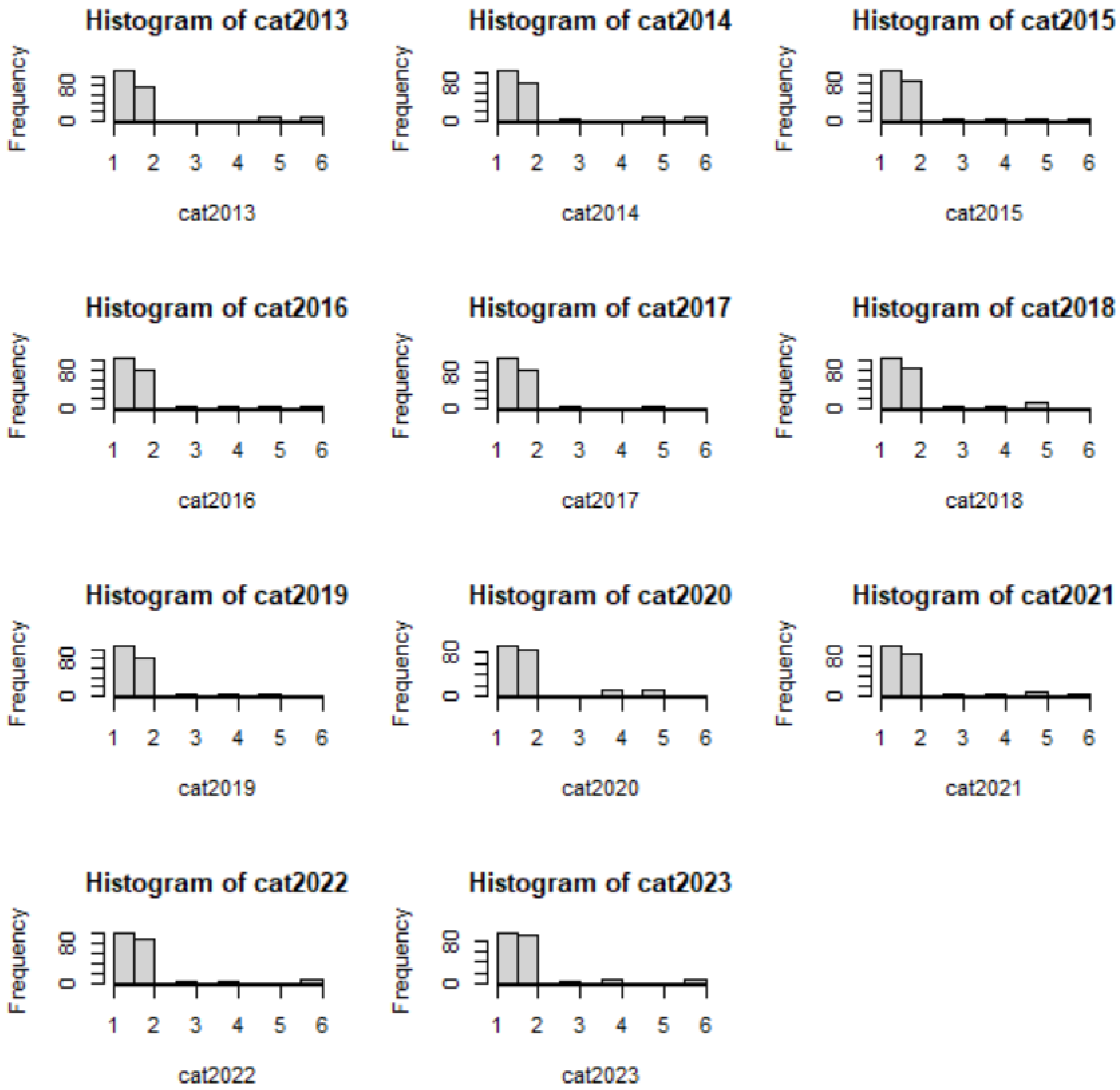
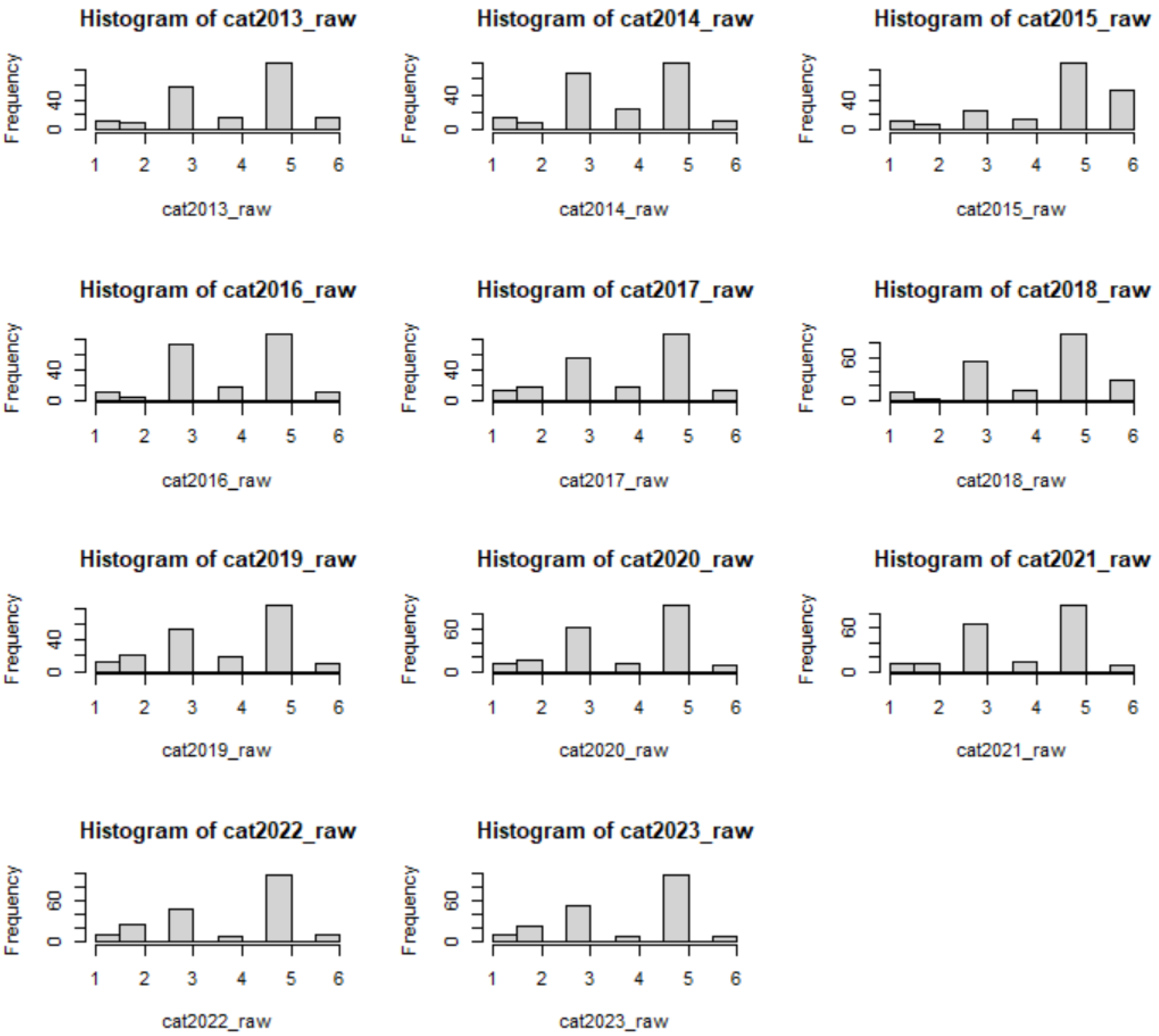
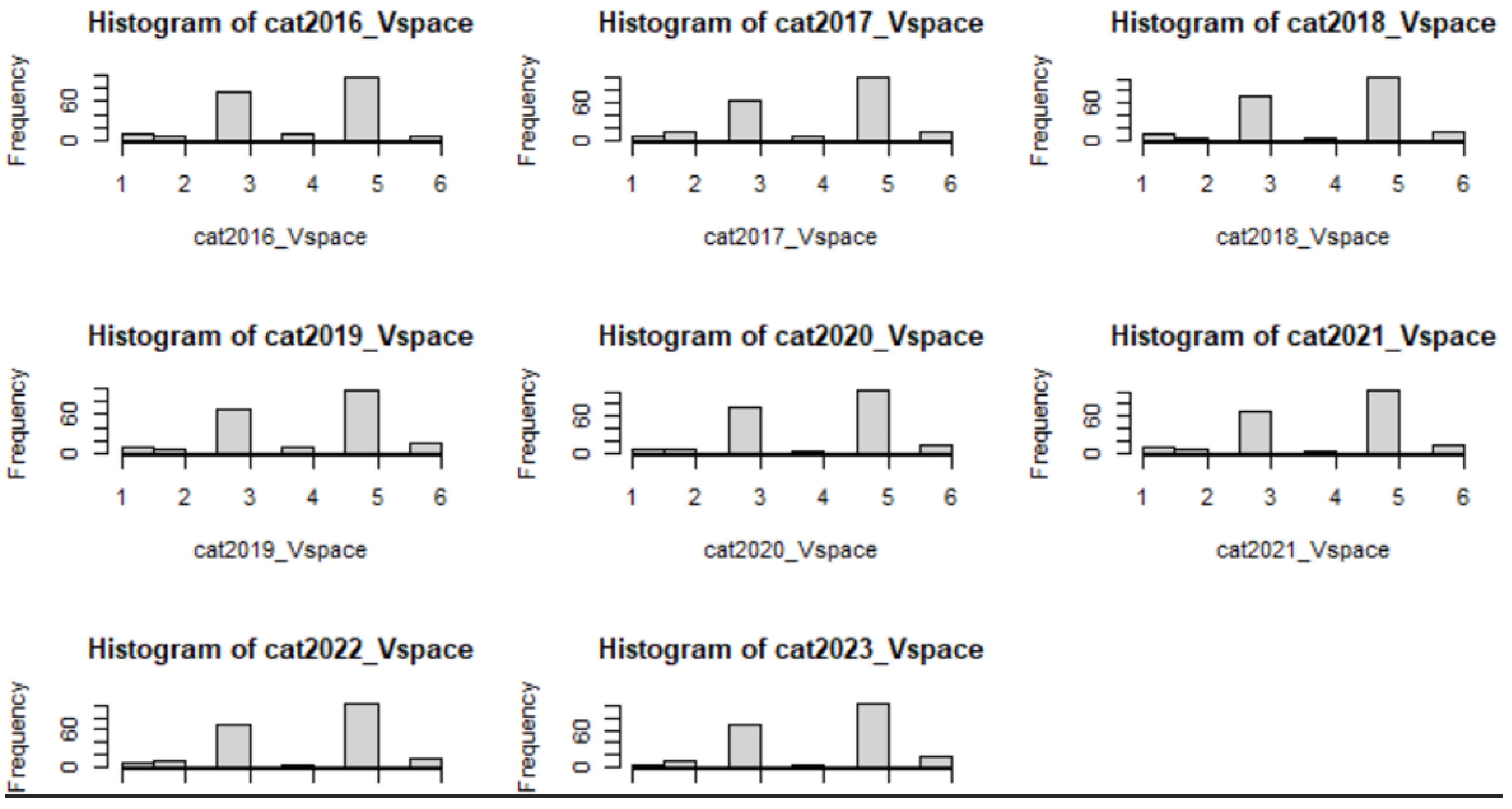
• Assign the categories (from 1 to 6) for each country by its maximal cosine value among all the 6 features. For each year t, find the positions (among columns) that yield the maximal values of $Co{s}_t$, row by row—let us name the categorization at year t by $Ca{t}_t$. For example, in the previous case, $Ca{t}_{2013}=\left[\begin{array}{c}ca{t}_{2013,1}\\ ca{t}_{2013,2}\\ ⋮\\ ca{t}_{2013,202}\end{array}\right]=\left[\begin{array}{c}1\\ 1\\ ⋮\\ 1\end{array}\right]$. The detailed categorization for all $Ca{t}_{2013},Ca{t}_{2014},\cdots ,Ca{t}_{2023}$ is presented in the Appendix A Listing A1. The categorization regarding the 6 representative countries is in particular singled out in Table 2. As for the statistics of the categorization distribution for the other countries, they are revealed in Figure 6.
  Table 2. The orthogonal features associated with each representative country from the year 2013 to 2023: The orthogonal features associated with each country are extremely stable—this indicates the governance systems in the representatives are consistent and also indicates their representations are reliable for the classification problem.

  Year	China	France	Germany	India	Russia	USA
  2013	1	2	2	1	1	2
  2014	1	2	2	1	1	2
  2015	1	2	2	1	1	2
  2016	1	2	2	1	1	2
  2017	1	2	2	1	1	2
  2018	1	2	2	1	1	2
  2019	1	2	2	1	1	2
  2020	1	2	2	1	1	2
  2021	1	2	2	1	1	2
  2022	1	2	2	1	1	2
  2023	1	2	2	1	1	2

  

  Figure 6. Frequency distribution of six categories from Year 2013 to 2023 by NsrGSP: These frequencies represent the relative proportion of countries that lie in each category. In total, there are six categories: 1, 2, 3, 4, 5, and 6. Each of the 202 countries were assigned a distinct category, and the overall distribution was captured by these histograms. The underlying method (NsrGSP) adopted is described as an algorithm in Section Application Two. The features for the six representative countries (China, France, Germany, India, Russia, and the USA) were further analyzed by another six orthogonal (hidden) features—one could regard these six new features as six new dummy countries. By associating (see Table 2) these new six dummy countries with the original six chosen representative countries, then some of the dummy countries become immediately explainable. Dummy Country 1 is associated with China, and Dummy Country 2 is associated with the USA—this is good since we could find the dominating factors/features/countries to represent the clustering/classification. These temporal histograms, which are named the Histogram of catxxxx, show that the China-style and USA-style governance systems are dominating this world, and there is no distinct difference for their domination.

Now let us do some evaluation and comparison regarding the classification problem with various methods based on cosine values and some bases. To this aim, together with our method (NsrGSP), we add two other approaches: one without any GSP involved (or NonGSP) and the other, with Classical GSP thought (or CGSP). The results for the NonGSP are shown in Figure 7. It shows the 3rd (Germany) and 5th (Russian) style governance systems dominate this world, and so does CGSP (the results are shown in Figure 8. Obviously this classification is not exactly what we anticipate—we would like the classification to preserve some distinct features that could differentiate it from another. This is achieved by NsrGSP, since the distinct features are now related to China and America, a result that could polarize the classification more.

Figure 7. Frequency distribution of the six categories from Year 2013 to 2023 by the nonGSP: These frequencies represent the relative proportion of countries that lie in each category. In total, there are six categories: 1, 2, 3, 4, 5, and 6. Each of the 202 countries were assigned a distinct category, and the overall distribution was captured by these histograms. The underlying method adopted was named nonGSP analysis (or nonGSP): the usual approach adopted in calculating cosine values to analyze the similarities between vectors/data. In our case, the representative vectors were six subjectively chosen countries (China, France, Germany, India, Russia, and the USA). Then, we calculated the cosine values of the 202 countries’ IDs with these six representative IDs and then picked up the most similar country (among the six representative countries) for each of the 202 countries. The results were then plotted as a histogram of $catxxx\_raw$, where raw means there is no further processing regarding the given IDs for the representative countries. From the temporal histograms, one could observe that Germany and Russia dominate the main representatives since their systems mix with various other factors that are also shared with other countries. Since their IDs were not further processed, such classification was less informative—we could not perceive the underlying differences easily.

Figure 8. Frequency distribution of the six categories from Year 2013 to 2023 by CGSP: These frequencies represent the relative proportion of countries that lie in each category. In total, there were six categories: 1, 2, 3, 4, 5, and 6. Each of the 202 countries was assigned a distinct category, and the overall distribution was captured by these histograms. The underlying method adopted was named Classical GSP analysis (or CGSP): this approach converts/projects all the original IDs into/onto the new (sub-)space spanned by the orthogonal vectors derived from the self-referential (or classical) GSP. The cosine values for the similarity computation are based on the coefficient vectors in this newly constructed space. Theoretically, it is appeasing; but experimentally, it has pretty much the same classifying results as nonGSP. It is also much more time consuming because we need to project the IDs of all the 202 countries onto the newly constructed space.

5. Conclusions

In this paper, we derived a non-self-referential inductive method for Gram–Schmidt processes based on the typical Gram–Schmidt process (TGSP). The main idea is to keep track of all indices of the TGSP and find the patterns of change between these indices. The results show that we could largely reduce the computational complexity of GSP and also keep the theoretical favor that all of the generated orthonormal vectors are non-referential. This will give us another perspective for GSP. The results show that

$$V_k=U_k{\left[\begin{array}{cc}{B}_{{\Delta }_{k-1}}^{+}& 0_{(k-1)\times 1}\\ U_{k-1}^{•}{(B_{{\Delta }_{k-1}}^{+})}^t({\displaystyle \frac{-1}{[U_{k-1}{(B_{{\Delta }_{k-1}}^{+})}^t]{\odot }_c[U_{k-1}{(B_{{\Delta }_{k-1}}^{+})}^t]}})B_{{\Delta }_{k-1}}^{+}& 1\end{array}\right]}^t,$$

where $k\ge 2$ and $B_{{\Delta }_1}^{+}=\left[1\right]$. Unlike another non-referential GSP or FDET (see Equation (1)), whose complexity is exponential due to the permutation, our method uses only polynomial complexity. This will bring some theoretical and practical advantages; for example, in Application Two, we showed it could provide a much more persuasive classification and could maintain the polynomial complexity. There are also some disadvantages to this approach. First of all, the presentation of our method is succinct, but the computation of the coefficients still needs to go through a set of recursive procedures. Secondly, we derive our method based on the classical GSP, which tends to cause computational error [12,13]. For a better performance, the readers could derive a new version of our method based on modified GSP [14,15]. Furthermore, it still needs more experiments and research on its applicability to other real-world problems.

References

- Deng, Y. On p-adic Gram–Schmidt Orthogonalization Process. Front. Math. 2024. [Google Scholar] [CrossRef]
- Huang, X.; Caron, M.; Hindson, D. A recursive Gram-Schmidt orthonormalization procedure and its application to communications. In Proceedings of the 2001 IEEE Third Workshop on Signal Processing Advances in Wireless Communications (SPAWC’01), Taiwan, China, 20–23 March 2001; Workshop Proceedings (Cat. No.01EX471). pp. 340–343. [Google Scholar]
- Balabanov, O.; Grigori, L. Randomized Gram-Schmidt process with application to GMRES. Siam J. Sci. Comput. 2022, 44, A1450–A1474. [Google Scholar] [CrossRef]
- Ford, W. Numerical Linear Algebra with Applications: Using MATLAB and Octave; Academic Press: Cambridge, MA, USA, 2014. [Google Scholar]
- Morrison, D.D. Remarks on the Unitary Triangularization of a Nonsymmetric Matrix. J. ACM 1960, 7, 185–186. [Google Scholar] [CrossRef]
- Skogholt, J.; Lil, K.H.; Næs, T.; Smilde, A.K.; Indahl, U.G. Selection of principal variables through a modified Gram–Schmidt process with and without supervision. J. Chemom. 2023, 37, e3510. [Google Scholar] [CrossRef]
- Robinson, P.J.; Saranraj, A. Intuitionistic Fuzzy Gram-Schmidt Orthogonalized Artificial Neural Network for Solving MAGDM Problems. Indian J. Sci. Technol. 2024, 17, 2529–2537. [Google Scholar] [CrossRef]
- Dax, A. A modified Gram–Schmidt algorithm with iterative orthogonalization and column pivoting. Linear Algebra Its Appl. 2000, 310, 25–42. [Google Scholar] [CrossRef]
- Trefethen, L.N.; Bau, D. Numerical Linear Algebra; SIAM: New Delhi, India, 1997. [Google Scholar]
- Bremner, M.R. Lattice Basis Reduction: An Introduction to the LLL Algorithm and Its Applications; CRC Press: Boca Raton, FL, USA, 2012. [Google Scholar]
- Available online: http://www.noahsd.com/mini_lattices/02__GS_and_LLL.pdf (accessed on 10 February 2025).
- Giraud, L.; Langou, J.; Rozložník, M.; Eshof, J.V.D. Rounding error analysis of the classical Gram–Schmidt orthogonalization process. Numer. Math. 2005, 101, 87–100. [Google Scholar] [CrossRef]
- Giraud, L.; Langou, J.; Rozloznik, M. The loss of orthogonality in the Gram–Schmidt orthogonalization process. Comput. Math. Appl. 2005, 50, 1069–1075. [Google Scholar] [CrossRef]
- Imakura, A.; Yamamoto, Y. Efficient implementations of the modified Gram–Schmidt orthogonalization with a non-standard inner product. Jpn. J. Indust. Appl. Math. 2019, 36, 619–641. [Google Scholar] [CrossRef]
- Sreedharan, V.P. A note on the modified gram-schmidt process. Int. J. Comput. Math. 1988, 24, 277–290. [Google Scholar] [CrossRef]