Article

Multi-Feature Extraction and Explainable Machine Learning for Lamb-Wave-Based Damage Localization in Laminated Composites

1
Department of Mechanical Engineering, Dongguk University-Seoul, 30 Pildong-ro 1-gil, Jung-gu, Seoul 04620, Republic of Korea
2
Department of Mechanical, Robotics and Energy Engineering, Dongguk University-Seoul, 30 Pildong-ro 1-gil, Jung-gu, Seoul 04620, Republic of Korea
*
Author to whom correspondence should be addressed.
Mathematics 2025, 13(5), 769; https://doi.org/10.3390/math13050769
Submission received: 2 January 2025 / Revised: 19 February 2025 / Accepted: 25 February 2025 / Published: 26 February 2025
(This article belongs to the Section E2: Control Theory and Mechanics)

Abstract

:
Laminated composites display exceptional weight-saving abilities that make them suited to advanced applications in aerospace, automobile, civil, and marine industries. However, the orthotropic nature of laminated composites means that they possess several damage modes that can lead to catastrophic failure. Therefore, machine learning-based Structural Health Monitoring (SHM) techniques have been used for damage detection. While Lamb waves have shown significant potential in the SHM of laminated composites, most of these techniques are focused on imaging-based methods and are limited to damage detection. Therefore, this study aims to localize the damage in laminated composites without the use of imaging methods, thus improving the computational efficiency of the proposed approach. Moreover, the machine learning models are generally black-box in nature, with no transparency of the reason for their decision making. Thus, this study also proposes the use of Shapley Additive Explanations (SHAP) to identify the important feature to localize the damage in laminated composites. The proposed approach is validated by the experimental simulation of the damage at nine different locations of a composite laminate. Multi-feature extraction is carried out by first applying the Hilbert transform on the envelope signal followed by statistical feature analysis. This study compares raw signal features, Hilbert transform features, and multi-feature extraction from the Hilbert transform to demonstrate the effectiveness of the proposed approach. The results demonstrate the effectiveness of an explainable K-Nearest Neighbor (KNN) model in locating the damage, with an R 2 value of 0.96, a Mean Square Error (MSE) value of 10.29, and a Mean Absolute Error (MAE) value of 0.5.

1. Introduction

Laminated composite materials have been widely used in big structures in industries such as aerospace, autos, wind power generation, railways, and high-technology ships. This is because laminated composites have high specific strength, stiffness, and mechanical qualities that can be designed [1,2,3]. The use of composite materials has proven to be a successful approach to reduce the weight of massive constructions while increasing efficiency and lowering running costs. However, laminated composites are susceptible to several damage types that include interlaminar delamination and cracking as a result of external stresses, production instabilities, temperature fluctuations, and humidity [4,5]. These damages typically begin as micro-cracks in the matrix and progress nonlinearly under cyclic loading. Interlaminar separation or delamination results in the ultimate failure of composite structures, while also significantly diminishing mechanical properties. Therefore, the reliability of composite structures is compromised, and safety is at risk due to the sudden failure that delamination in composite materials can cause. Thus, to avoid severe catastrophes and prevent subsequent deterioration in structural performance, it is important through timely maintenance to identify interlaminar delamination at an early stage [6,7]. Consequently, to facilitate the timely identification of structural damage and to facilitate the implementation of appropriate maintenance, a Structural Health Monitoring (SHM) system is essential [8,9]. The SHM system helps prevent sudden failure and extends the lifespan of composites. Therefore, to prevent structural failure and sudden damage, it is crucial to promptly identify damage in composite structures [10,11].
SHM technology is a revolutionary and innovative technique for composite structure health assessment [12]. Lamb-wave-based SHM techniques have been widely documented to be sensitive to tiny damage, are easily accessible, and are efficient in the identification of fatigue cracks in metallic structures, debonding and delamination in composite structures, and the assessment of structural repairs [13]. Thus, through the application of SHM technology, numerous methodologies have been employed to identify and localize damage in composite structures [14,15]. Lamb wave detection has become a viable technology to detect damage in composite structures. Its capacity for low attenuation, expansive detection coverage, long-range propagation, and great sensitivity to mild damage have resulted in it attracting considerable attention in damage localization [16,17,18]. The detection technology uses surface-attached sensors to monitor the structure in real time. Piezoelectric transducers (PZTs) are frequently employed to produce and obtain Lamb wave signals [19,20]. The impact of the sensor array must be carefully studied to ensure accurate damage localization for Structural Health Monitoring.
SHM technology that uses Lamb wave detection is classified into two types: physics-based and data-driven [21]. Physics-based models use mathematical representations of the physical principles and working mechanisms of a system to predict damage and degradation processes. Equations or physical phenomena that represent the real damage mechanisms taking place within the system are used to describe how the system performance deteriorates. Time of Flight (ToF), Finite Element Analysis (FEA), and Paris’ Law provide a few instances of physics-based models [22,23]. Because they are grounded in the physical knowledge of the damage process, the results of these models are easily explained. Furthermore, even with a small amount of measurement data, they may use simulations or physical equations to produce steady and predictable results. However, these models necessitate intricate mathematical modeling and a thorough comprehension of the workings of the system. Altering the system setup, or unforeseen environmental changes taking place, might decrease their forecast accuracy [24]. In contrast, data-driven models use extensive data to predict health states and examine patterns of damage and degradation within the composite structure. The data-driven models, which depend on statistical techniques, machine learning, and deep learning, make predictions from the gathered data without necessitating the thorough comprehension of the actual behavior of the system [25]. Data-driven models have the advantage of being able to learn a variety of data patterns, which makes them useful in settings where physical models can be difficult to use or are constrained. When there is a sufficient amount of training data, data-driven models can attain high predicted accuracy [26,27]. However, adequate data are necessary for accurate predictions, while insufficient data might result in problems like overfitting. Among data-driven approaches, machine learning techniques are very helpful in identifying patterns through feature extraction from the data. These methods are frequently used in a variety of SHM domains, such as anomaly identification in systems, predictive maintenance, and damage detection [28].
Accurate damage localization in composite materials is significantly difficult, along with making the machine learning approaches interpretable. Therefore, based on envelope properties and statistical features in a machine learning model, this research suggests a technique for locating damage using Lamb wave signals obtained from laminated composite structures. To validate the suggested approach, an experimental system with four PZT sensors was used to gather Lamb wave signals, and its performance in detecting damage in laminated composite constructions was evaluated. To train a model that achieves high accuracy in estimating damage locations, it is necessary to extract several statistical features from the collected dataset that assist damage localization in laminated composites. The Lamb wave signals are normalized to reduce signal differences. A Hilbert transform is used to extract the envelope signal from the raw signal, and then statistical properties are applied to the extracted envelope signal to obtain features that can be used to train machine learning models. These characteristics help the machine learning model function better by offering vital information to more precisely estimate the location of damage.
Additionally, black-box machine learning algorithms can be risky in high-stakes decision making. They rely on untrustworthy databases, making real-time forecasts difficult to troubleshoot, explain, and test for errors. Their use presents serious ethical and accountability issues [29]. To solve this problem, by applying the SHAP method, the significance of statistical features is determined, and these features are utilized to understand the black-box characteristics of the machine learning model and assess the influence of each feature on predictions [30,31]. This strategy improves the machine learning model’s explainability and transparency, increasing the reliability of the results and allowing for data-driven decision making in model evaluation and management [32]. The retrieved characteristics improve the model’s overall performance by increasing its explainability and providing a deeper knowledge of how it discriminates between different damage locations. This study advances the field of damage detection in composite materials by not only detecting the presence of damage and predicting its position, but also by incorporating SHAP to improve the explainability and reliability of the findings. Accurate damage localization in composite materials is very difficult, and the multi-feature extraction method suggested in this study could greatly improve accuracy.
The structure of this paper is as follows: Section 2 provides the experimental setup and methodology of this paper. In Section 3, hyperparameter optimization, evaluation metrics for five machine learning models, and Explainable Artificial Intelligence are discussed. Section 4 discusses the conclusion of this work and future work in damage localization.

2. The Proposed Methodology

Figure 1 shows the comprehensive approach to the localization of damage in composite structures using Lamb wave data that the proposed methodology involves. Initially, Lamb wave signals are acquired through an experimental setup, where signals are propagated through the composite material. The raw data undergo normalization, followed by a path fusion process to integrate data from 12 paths for accurate damage localization. A PZT sensor with three paths monitors each damage location, while a total of four PZT sensors are placed at the edges of the composite laminate, resulting in twelve data paths. After path fusion, the Hilbert transform is applied to extract envelope signals for further analysis. A set of statistical and signal-based features that include mean, standard deviation, root mean square, skewness, kurtosis, peak-to-peak, crest factor, impulse factor, margin factor, and shape factor are extracted from the processed data. These features are then used to train various machine learning models that include Support Vector Regression (SVR), Random Forest (RF), Bayesian Ridge (BR), Decision Tree (DT), and K-Nearest Neighbor (KNN) to establish relationships between the extracted features and damage metrics. The KNN model is used to localize damage, while SHapley Additive exPlanation (SHAP) is employed to explain the damage by analyzing the importance of features and gaining insights into the decision-making process of the model. This approach allows for accurate damage localization and a better understanding of the underlying patterns within the data.

2.1. Damage Simulator

Data Acquisition from the Damage Simulator

Epoxy-based carbon fiber prepreg (T700SC-12k-60E), which has a high strength-to-weight ratio and superior mechanical qualities, was utilized to produce the composite plate employed in this study. The prepreg was made of carbon fibers that had already been coated with epoxy resin; so, during the fabrication process, the resin content and fiber alignment could be precisely controlled. As seen in Figure 2, the composite layup of eight [0/90/0/90]s plies was organized in a symmetric cross-ply pattern. The initial coupon measurements for composite laminate were 35 cm × 35 cm, guaranteeing there would be sufficient material for additional testing and processing. These composite laminates were created using a hot press machine, with the curing cycle following the guidelines supplied by the material supplier. Specifically, the laminates were cured at 120 °C under 20 kg/cm2 pressure for 3 h. Figure 2 displays the composite sheet created with this method. After their rough edges were cut off, bringing the coupon measurements down to 30 cm × 30 cm, the created laminates were used in this study for additional testing and assessment.
Data were collected using Lamb wave tests from the trimmed composite sheet. Figure 1 shows the experimental setup, which consisted of an amplifier, a data acquisition (DAQ) device, a composite specimen with a PZT sensor array, and a LabVIEW PC for generating Lamb waves, displaying signals, and storing sensor data. An NI USB-6341 DAQ was used to excite the PZT and regulate the working sequence of every PZT pair, while a PZD700A dual-channel amplifier was employed to enhance the excitation signal. Four PZTs from PI Ceramic were glued to the composite laminate in an orthogonal pattern, and a small cylindrical mass was attached to simulate the damage. In addition, the damage was simulated at nine distinct locations on the composite sheet to provide localization data. Figure 3 displays a schematic of the damage simulator. MATLAB R2022b’s analog output generator was used to generate the excitation signal, which consisted of a 5-cycle sinusoidal tone burst with a center frequency of 150 kHz, and was windowed using a Hanning function. Before being sent to the PZT, the burst signal was amplified using a power amplifier to a level of 50 Vpp. During the experiments, three PZTs worked as sensors in this configuration, catching the Lamb wave signals actuated from the remaining PZT. Figure 3c shows that this procedure was methodically repeated for each of the four PZTs, with each PZT acting, in turn, as the actuator. The distance between the PZT sensors was 24 cm. This created a total of 12 distinct sensing routes. To create a complete dataset across the orthogonal arrangement, an NI USB-6341 data-gathering device was used to capture these 12 propagation routes at a sampling frequency of 500 kHz for each damage location. For each scenario, the signal acquisition was repeated 30 times to verify experimental reproducibility. The experiments were conducted in sequence from L1 to L9 for the nine locations as shown in Figure 3, and the 12 sensing routes were determined by conducting tests consecutively from PZT sensor 1 to PZT sensor 4. Figure 3c shows detailed information regarding the routes. This resulted in the gathering of 600 (12 paths × 50 repetitions) healthy signals and 3240 (12 paths × 30 repetitions × 9 locations) damaged signals. To validate the suggested method, training and test datasets were divided in an (80:20) split. For each damage location, 360 Lamb wave signals were collected, and the data from each of the nine damage locations were randomly split into training (80%) and test (20%) sets. This means that the data were not randomly split as a whole, but, rather, individually for each damage location. Additionally, all 600 healthy signals were included in the training set. As a result, the final training dataset contained 2592 damage signals and 600 healthy signals, while the test dataset consisted of 648 damage signals.
The experiments were conducted to ensure that data for each damage condition were collected evenly, and the damage classes were evenly distributed before splitting the dataset into an 80:20 ratio. Before creating the model, all the data were normalized to the range of −1 to 1, while, during evaluation, they were rescaled to pinpoint the precise region of the damage.

2.2. Hilbert Transform

The obtained response signals were normalized and analyzed in the temporal domain to enhance the analysis of guided wave propagation properties in laminated composites. Even though time domain analysis can be used to observe the overall variation trend of the response signals, the unique characteristics of guided waves cannot be sufficiently defined [33]. This is addressed by using the Hilbert transform method to transform the raw signal into a complex analytic signal, which yields both the original signal and a phase-shifted version [34]. This modification makes it possible to perform additional analyses, such as extracting the envelope and instantaneous phase of the signal [35]. The following are specific formulae for Hilbert transformations.
Equation (1) represents the continuous-time Hilbert transform, expressed as an integral over an infinite domain.
H [ x ( t ) ] = x ^ ( t ) = 1 π + x ( τ ) t τ d τ
The inverse transformation of Equation (1) is as follows.
x ( t ) = H [ ( x ^ t ) ] = 1 π + x ^ ( τ ) t τ d τ
An analytical signal for the complex conjugate pair x ( t ) and x ^ ( t ) is as follows:
z ( t ) = x t + j x ^ t = a ( t ) e j θ ( t )
where x ( t ) is any continuous transient signal, θ ( t ) is a phase, α ( t ) is an instantaneous amplitude, and x ^ ( t ) is a complex signal following the Hilbert transform.
The formula for calculating the instantaneous amplitude and phase is as follows.
a t = x 2 t + x ^ 2 t
θ t = t a n 1 ( x ^ t x t )
To properly describe this pattern, the Hilbert transform is used to extract the signal’s envelope.

2.3. Multi-Feature Extraction

Statistical characteristics help the model learn and comprehend the general patterns in the data by condensing important information from the data. By condensing the data into a lower-dimensional form, statistical characteristics also contribute to lower computational costs and increased training efficiency [36]. In addition to helping comprehend the model’s predictions, statistical features are easily understood intuitively, which enhances model performance. By using statistical features instead of raw data, the model can converge more quickly, and attain higher accuracy. In this study, multi-feature extraction was performed over the entire time window of the signal. Mean, standard deviation, skewness, and kurtosis are features related to the central tendency and distribution of the data, whereas root mean square, peak, and peak-to-peak are energy- and amplitude-based features. Additionally, shape-related factors include shape factor, crest factor, impulse factor, and margin factor. Skewness, kurtosis, and crest factor are examples of specialized statistical traits that might be crucial in certain applications, such as damage diagnostics [37,38]. For example, typically, the mean value of vibration data is zero. However, in real-time monitoring, it frequently deviates and varies close to zero due to a variety of factors such as noise, weather conditions (e.g., wind, rain, and temperature fluctuations), or natural structural changes over time. Furthermore, large events such as earthquakes can cause inelastic deformations, resulting in persistent variations in the mean value. Thus, the reliable tracking of changes in the mean value is critical for successful monitoring and analysis [39]. Standard deviation is a widely known and validated statistical method used to reduce the size of data without losing their meaning [40]. It is commonly utilized in statistics and probability theory as a measure of variability or diversity. It indicates how much values deviate from the ‘average’ (expected value) [41]. Skewness is a statistical term that assesses the asymmetry of a signal’s distribution concerning its mean. It has a high sensitivity in several data processing applications and has been intensively utilized to improve the resilience of statistical parameters [42]. Kurtosis is a statistical measure that compares the weight of a probability distribution’s tails to that of a normal distribution [43]. This feature gives information about the signal distribution by determining whether it is sharp and abrupt or generally flat. It also exposes changes in the form of guided wave signals, notably in the first wave packet, when the propagation path between two transducers passes through a damaged area [44]. It is especially useful for defining sparse data because the empirical distribution has just a few notable peaks, resulting in high kurtosis values [45]. Therefore, kurtosis has been used for the identification of localized damages [46]. Table 1 lists, briefly explains, and mathematically expresses the features retrieved from the time domain data [47,48,49].

2.4. Machine Learning Models

2.4.1. Decision Tree

DT regression is a form of DT classifier that is intended to predict real-valued outcomes, like class proportions [50]. Figure 4 shows the structure of a DT regression and its recursive binary splitting process. The repeated process of binary recursive partitioning, which divides data into partitions, is also used to construct a regression tree. The initial step is to create a tree structure that utilizes all the training data. The method assesses each alternative binary split, separating the data into two parts, and, in each subset, chooses the split with the lowest sum of squared deviations from the mean. The splitting process is then repeated for each new branch. The technique is repeated until each node reaches a user-defined minimum size (i.e., the number of training samples), at which point it becomes a terminal node. Once the entire structure is acquired, the tree may experience overfitting because it was constructed using training data. When used on unseen data, this could reduce the tree’s classification accuracy and limit its capacity for generalization. As a result, a pruning process is typically carried out, employing a validation dataset and a user-defined cost complexity parameter. Pruning reduces the variance of the output variable in the validation data, as well as the product of the number of terminal nodes and the cost complexity factor, which indicates the node’s complexity cost. During the pruning process, the last node to be added is deleted first, followed by the next.

2.4.2. K-Nearest Neighbor

K-Nearest Neighbor (KNN) regression is a strategy used to predict the value of a target variable for a new data point based on the nearest points in the dataset [51]. Both the training and test datasets are used to gather observational features. The technique can be expanded to include additional predictors, even though the data may only be represented by two features on a two-dimensional graph. The fundamental idea underlying KNN regression is to determine the distance between data and to estimate the target variable using either a simple average or a distance-weighted approach based on the K-Nearest Neighbors [52]. Figure 5 shows how KNN employs proximity to predict target values based on neighboring data points. The Euclidean distance, which is defined as follows, is a widely used method for calculating distance in KNN [53,54,55]. Therefore, it has been used in this study. The Euclidean distance can be expressed as follows.
D ( p , q ) = ( p 1 q 1 ) 2 + ( p 2 q 2 ) 2 + + ( p n q n ) 2
In this case, n is the number of features, and p and q are the data points under investigation. The Euclidean distance was used as the major distance measure in this study because it is computationally simple and effective to estimate straight-line distances in a multidimensional environment. While other distance measures, such as the Manhattan distance, might have been employed, the Euclidean distance was chosen since it closely matches the properties of the dataset utilized in this study [56,57]. K is another crucial parameter in the KNN algorithm that establishes how many neighbors to consider. The value of k greatly impacts the performance of the algorithm. While a higher k decreases variance due to random errors, it may overlook more significant smaller patterns. On the other hand, a lower k runs the risk of overfitting, but is more responsive to local patterns. When choosing k , it is crucial to strike a balance between overfitting and underfitting. Generally, k is set to the square root of the observation count of the training dataset [58,59].
Figure 5. KNN regression method showing how proximity to neighbors predicts target values.
Mathematics 13 00769 g005

2.4.3. Random Forest

RF is an ensemble of random DT classifiers that combine their predictions and is distinguished by how randomness is injected into the tree-building process. This paper specifically considered the RF approach created by Breiman [57], which integrates bagging with random feature selection [60]. More formally, a bootstrap approach is used to generate several randomized training sets by sampling with replacement from the initial training set, guaranteeing that each bootstrap sample has the same number of occurrences as the original set. The random DT learner is characterized by a positive integer parameter in the range (1 ≤ v < d). The tree is constructed by recursively splitting the instance space. Each stage of the tree’s development involves evenly and randomly selecting v variables from the d candidates, x(1), …, x(d). If each cell uses a majority vote, the leaf node is then split using one of these v variables to reduce the misclassification of training points. The process is repeated until all the cells are pure. Figure 6 illustrates the RF model.

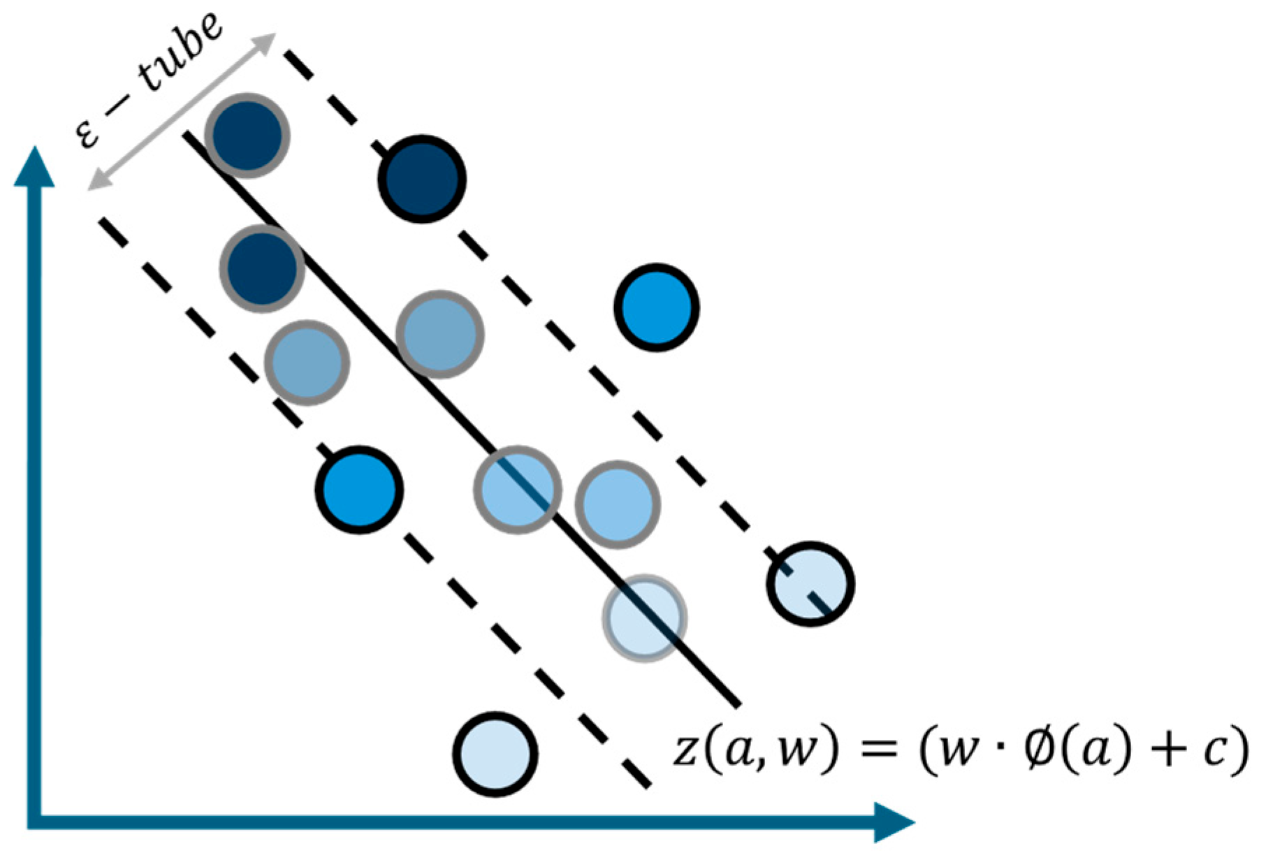
2.4.4. Support Vector Regression

SVR is a well-known approach to predict and fit curves in linear and nonlinear regression. SVR is based on Support Vector Machine (SVM) principles, in which support vectors are the points closest to the hyperplane in an n -dimensional feature space, allowing data points to be successfully separated with regard to the hyperplane [61]. Figure 7 shows how the SVR model conducts the fitting. Regression is based on the following training data: P = { a 1 , b 1 , a 2 , b 2 , , a N , b N } , where a i represents a vector of real-valued independent variables, whereas b i is the equivalent real-valued dependent variable. The hyperplane equation can be expressed in the following form:
z a , w = ( w · a + c )
where ( w · a ) is the dot product therein, x is the feature function, w is the weight, and b is a constant. The following equation minimizes the objective function.
M i n i m i z e : Q f = C 1 N L ε ( b , z ( a , w ) ) + 1 2 w 2
L ε b , z a , w =           0                                                     i f       b z ( a , w ) ε b z ( a , w ) ε                               o t h e r w i s e
The term on the left side of Equation (7) indicates the empirical error, whereas the constant C quantifies the trade-off between the empirical error and model complexity, which is described by the second term of the equation. Equation (8) defines the ε -insensitive loss function [62]. By adding Lagrangian multipliers β and β * , the optimization problem is converted into its dual form. Only the non-zero coefficients are referred to as support vectors, together with their input vectors, a i . The completed form appears as follows.
z a ,   β i , β i * = i = 1 N s v ( β i β i * ) ( a i · a j ) + C
The kernel function K ( x i , x j ) can be used to obtain the SVR function, which is given by the following.
a , β i , β i * = i = 1 N s v ( β i β i * ) K ( a , a i ) + C
The Karush–Kuhn–Tucker conditions are used to calculate the term, C .

2.4.5. Bayesian Ridge

BR regression combines elements of the Bayesian approach and ridge regression [63]. The Bayesian technique first uses the likelihood function to evaluate information about the dataset distribution, known as the prior distribution of parameters. Bayes’ theorem is used to generate a posterior distribution for the prediction of unknown scenarios, as shown in Equation (11).
P ( θ | x ) P ( x | θ ) P ( θ )
The posterior distribution is denoted by P ( θ | x ) , the likelihood function by P ( θ | x ) , and the prior distribution by P ( θ ) . Except for straightforward situations, evaluating posterior distribution data is typically challenging. For complex situations, the Markov Chain Monte Carlo technique is employed to obtain the posterior distribution. The multicollinearity component of the dataset is handled by the ridge regression portion of the model. Assume that the data M j t possesses multicollinearity for a function (12). Conventional analytical methods, such as the ordinary least squares approach, would result in inaccurate variable inference for such a dataset.
a j t = M j t γ t
However, ridge regression will increase the accuracy of regression parameter estimations by adding a tiny bias. An exchangeable prior distribution is applied to the components of the regression vector in the ridge regression method, which is a version of the classic posterior Bayes regression [64]. However, a preliminary standardization procedure is necessary to make this assumption credible. This entails applying Equations (13) and (14) to standardize the variables Z j t and their related coefficients γ t . Consequently, a j t now becomes Equation (15) [65,66].
Z j t = ( M j t M ¯ j t ) s d ( M j t )
γ t = b t s d ( M j t )
a j t = M j t b t

2.4.6. Explainable Machine Learning

While Explainable Artificial Intelligence (XAI) lacks a broadly accepted definition, it is commonly viewed as a collection of tools or procedures that aim to clarify how model predictions are made [67,68]. XAI approaches can be classified according to model explainability, application domain, and scope of use. Explainability can be approached in two ways: models that are intrinsically explainable owing to their structure and simplicity (model-based), and those that require extra procedures to explain their predictions after the model has been trained (post hoc) [69]. Some XAI techniques are model-agnostic, meaning they can be used with any kind of machine learning model, regardless of its features. On the other hand, some strategies are model-specific, only working with certain types of models. Finally, XAI can be classified according to its scope, which can range from explaining the entire model (global explanation) to explaining certain components or individual model predictions (local explanation). Two extensively used XAI strategies in ML are SHAP [70] and Local Interpretable Model-agnostic Explanation (LIME) [71]. While LIME focuses on local explanations, SHAP provides a more comprehensive understanding by combining local observations with global perspectives. It achieves this by comparing individual predictions to the aggregate average prediction. On the other hand, LIME works under the assumption that, while a model may appear complex when seen globally, it can be represented by a linear model at the local level. LIME generates slightly modified instances close to the target data point, which are then fed into a black-box machine learning model to provide predictions. LIME then uses basic interpretable models, like linear regression, Least Absolute Shrinkage and Selection Operator (LASSO), or Decision Trees, to provide parameters that help explain the results. On the other hand, SHAP computes Shapley values to determine how each feature contributes to predictions based on selected data points. Unlike SHAP, LIME generates synthetic data by taking into account nearby instances, rather than the actual feature value of the instance being explained [72]. In contrast, the SHAP value is often regarded as a reliable indication of feature importance. Considering the aforementioned characteristics, the authors elected to employ the SHAP explainable model in this work to better comprehend the ML model predictions.

2.4.7. SHAP

The model results were initially explained using the Shapley Additive Explanations algorithm. SHAP is a game-theory-based strategy to improve the explainability of the results of machine learning models [73]. Complex mathematical methods are used to achieve this, giving each feature a value that is then increased or decreased depending on how much each feature contributed overall to the prediction. Each iteration in the dataset is subjected to this process; the final number assigned to each feature indicates how important it is to the overall classification of the data. This approach was selected above other explainability techniques because it can fully explain the relationship between the model output and the global average for a given explanation. Although SHAP takes a lot longer than other algorithms to analyze every potential prediction for a given instance with every possible input combination, it often results in higher local accuracy.

2.4.8. Evaluation Metrics

The performance of the model was evaluated using the following three metrics: correlation coefficient ( R 2 ), Mean Square Error (MSE), and Mean Absolute Error (MAE) [74,75]. Their expressions are as follows:
R 2 = ( n y i y ^ y i y ^ ) 2 [ n ( y i 2 ) ( y i ) 2 ] n [ ( y ^ 2 ) ( y ^ ) 2 ]
M S E = 1 n i = 1 n ( y i y ^ ) 2
M A E = 1 n i = 1 n y i y ^  
where n is the number of samples, y i is the experimental compressive strength value, and y ^ is the projected value.

3. Results and Discussion

3.1. Grid Search Hyperparameter Optimization

Grid search [76] is a popular method for hyperparameter optimization, which is a crucial process in machine learning. The aim of hyperparameter optimization is to find the ideal combination of hyperparameters that produce the best model performance on a validation set. The grid search process is to inspect a preset set of hyperparameters to identify the greatest combination that produces the best outcomes. Grid search determines the combination of hyperparameters that produces the best results by analyzing the performance of the model for each combination within a given range. Grid search can be computationally expensive because it requires training and evaluating the model for several hyperparameter combinations. However, the performance improvements obtained through the grid search method make the additional computational time worthwhile. Thus, in this study, the grid search process was used to optimize the hyperparameters of the machine learning models that were used. Table 2 shows the hyperparameter optimization process for the five machine learning models.

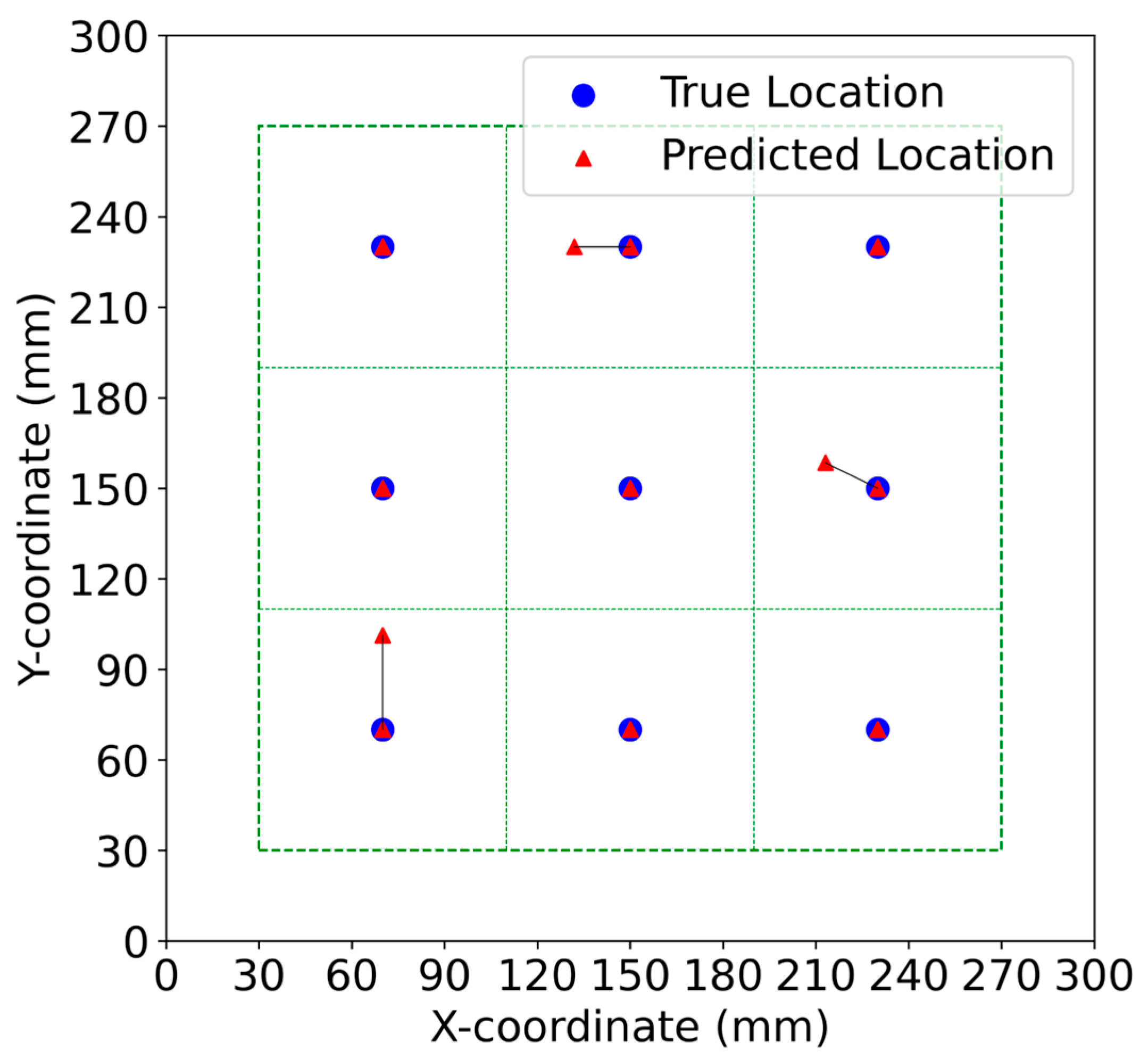
3.2. Damage Localization

To quantify damage localization performance, three sets of features were examined: raw signal features, Hilbert transform features, and multi-feature extraction from the Hilbert transform. The findings provide MSE, MAE, and R 2 values for the five models: BR, RF, SVR, DT, and KNN. Figure 8 compares the performance of the five machine learning models with characteristics retrieved from raw signals in terms of the (a) MSE, (b) MAE, and (c) R 2 values. The RF model shows the lowest MSE (159.1) and MAE (5.58), with an R 2 value of 0.83, indicating good performance. KNN performed well with an R 2 value of 0.89, but its MSE (176.3) was slightly higher. SVR performed poorly, with an R 2 of 0.36. Among the three feature sets, multi-feature extraction from the Hilbert transform yielded the best overall performance across most models, demonstrating its effectiveness in capturing critical damage localization patterns. Models trained on these multi-extracted features showed lower MSE and MAE values, along with higher R2 scores, indicating improved predictive accuracy and robustness. In contrast, Hilbert transform features alone resulted in the weakest performance, particularly in models like SVR, suggesting that relying solely on transformed features may lead to information loss or inadequate representation of underlying signal characteristics. The multi-feature extraction from raw signals ranked second, outperforming single-feature sets but falling short of the multi-feature extraction from the Hilbert transform. These results emphasize the critical role of multiple feature extraction in enhancing machine learning model performance, as it enables richer signal representation and improves accuracy in damage localization tasks.
Table 3 presents the evaluation metrics of the proposed multi-feature extraction and machine learning-based defect diagnosis model, which demonstrated high consistency. This consistency indicates that the model has stable generalization performance. It shows that effective feature extraction and model construction can minimize prediction variability.
Figure 9 shows the performance of the machine learning model using the Hilbert transform, where subfigures (a), (b), and (c) show the MSE, MAE, and R 2 values, respectively. In this instance, the KNN model performed noticeably better than the other models, with an MSE of 40.12, MAE of 1.48, and R 2 value of 0.91. RF also showed reasonable performance for damage localization in laminated composites, with an R 2 value of 0.87. However, BR showed the lowest accuracy with an R 2 value of 0.16. Figure 10 compares the performance of the models employing multi-feature extraction from Hilbert transform. The multi-feature extraction method improved the damage localization performance, especially for KNN, which attained the best accuracy with an MSE of 10.29, MAE of 0.5, and R 2 value of 0.96. RF showed an R 2 value of 0.91 and MSE of 52.51, while the SVR model showed the worst performance, with an R 2 value of 0.3 and MSE of 1731.43. Therefore, the results in Figure 8, Figure 9 and Figure 10 show that KNN consistently outperformed the other models, with significant improvements in damage localization when applying the Hilbert transform and its multi-feature extraction. These results highlight the importance of feature engineering in improving the performance of machine learning models for the SHM of laminated composite structures.
Figure 11 illustrates the damage localization prediction results using the KNN model with multi-feature extraction from the Hilbert transform. This graph visually presents the results of the test dataset, comparing the true damage locations (blue circles) with the predicted locations (red triangles) on a 300 mm × 300 mm coordinate grid. The plot area is divided into a 3 × 3 grid using green dashed lines for better visualization. Nine damage locations were tested and, in most cases, the predicted locations demonstrated very close alignment with the true locations, with only minor deviations observed in a few points, particularly in the upper middle region. This visual representation confirms the high accuracy of the KNN model using multi-feature extraction from the Hilbert transform, which, among the tested models, achieved the best performance metrics.

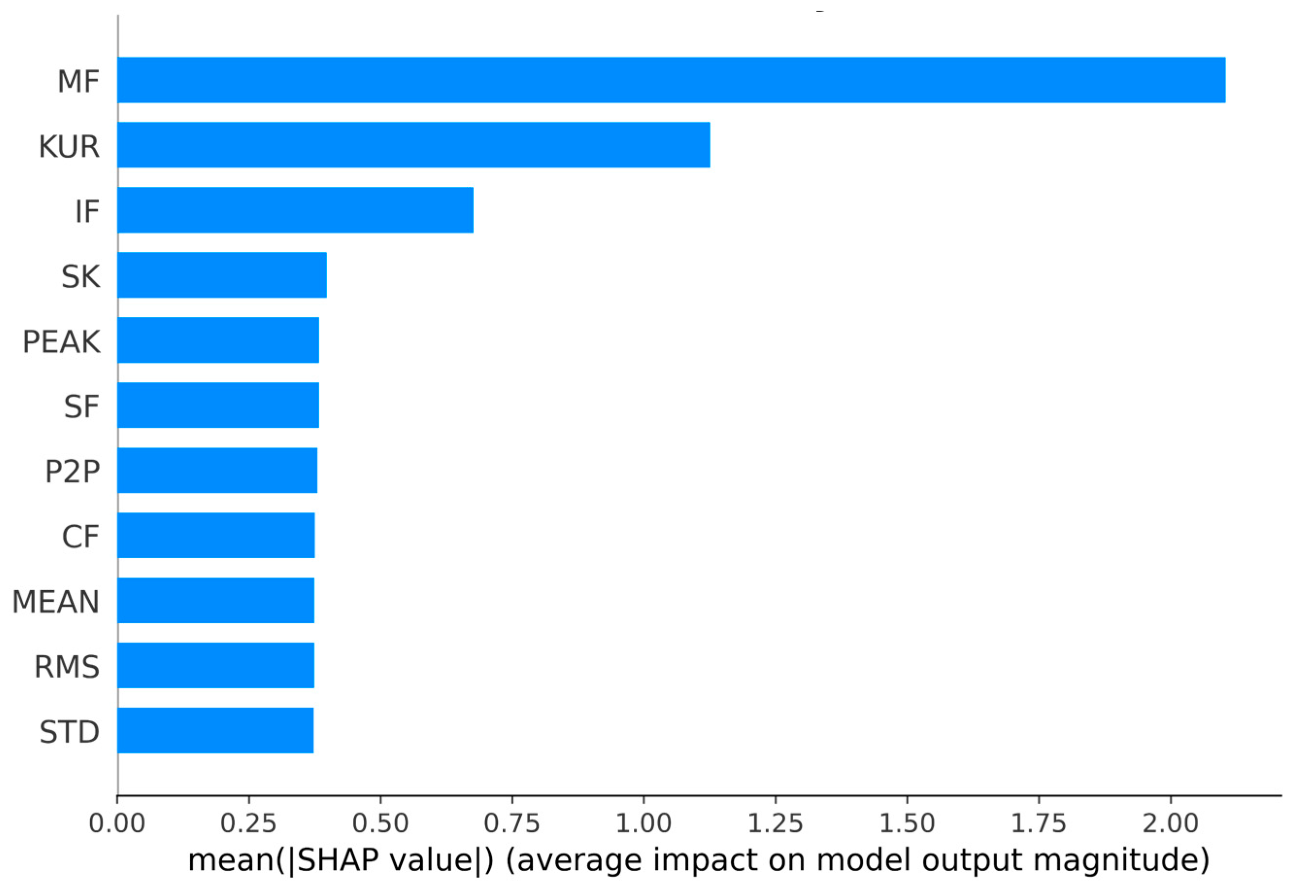
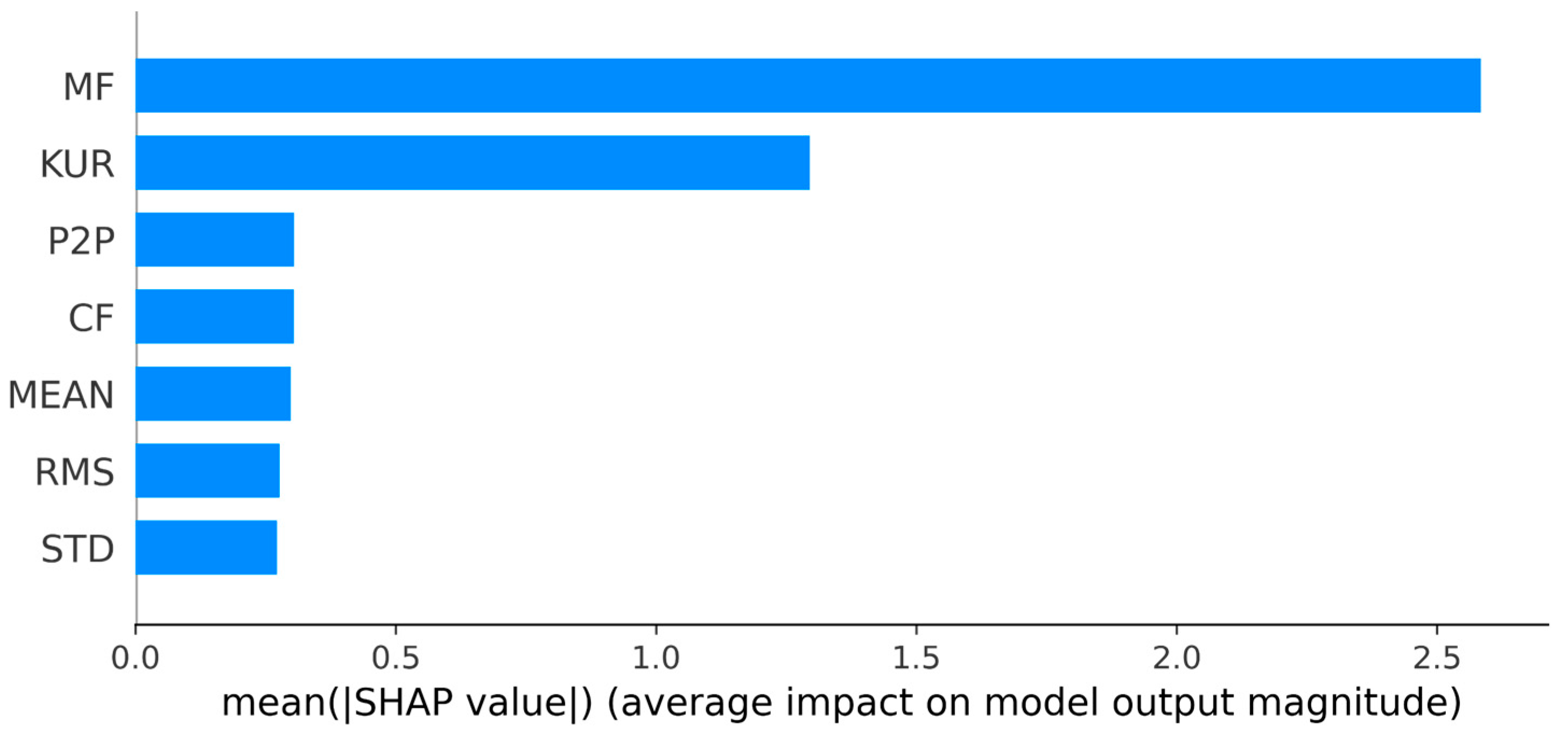
3.3. Explainable HT−MFE

After using the Hilbert transform to extract the envelope of Lamb wave signals from the laminated composites, statistical features (e.g., mean, standard deviation, skewness, and kurtosis) were obtained. These features were then used for damage localization via the KNN model that showed the highest localization performance, and SHAP analysis was conducted to visualize the importance of each feature. The margin factor is sensitive to variations in the signal generated by flaws, increasing the efficiency of defect identification. Kurtosis increases when a fault occurs, since the signal exhibits sudden changes or outliers. Therefore, Figure 12 shows that the margin factor and kurtosis emerged as the most influential features in predicting damage locations, with SHAP values of approximately (2.1 and 1.13), respectively. Other features, such as impulse factor and skewness, also significantly contributed to the decision-making process of the KNN model. The SHAP analysis highlights the critical role of the margin factor and kurtosis in the accurate damage localization of laminated composites, highlighting their significance in enhancing the explainability of the KNN model. These findings validate the effectiveness of statistical feature selection in improving both the model performance and decision transparency.
The correlation analysis revealed that there was a high correlation between SF, IF, and MF, as well as between SK and KUR. Additionally, there was a high correlation between peak and P2P. As a result, four features (SK, SF, IF, PEAK) were excluded, and the model was trained using the remaining seven features (MEAN, STD, RMS, KUR, CF, MF, P2P). Subsequently, SHAP was used to analyze the importance of the features, and the analysis showed that MF and KUR had the highest feature importance, as shown in Figure 13. Also, the performance of the model was evaluated, resulting in an MSE of 47.29, MAE of 1.71, and R2 of 0.95, similar to when all 11 features were used for training.
Based on this study, future research will focus on real-time feasibility. Furthermore, limiting the amount of features had no significant impact on the assessment metrics, which may assist in reducing the computational complexity of feature extraction and prediction methods. Furthermore, to assess the feasibility of a real-time damage location tracking system, the processing speed and latency will be evaluated and compared against the real-time requirements of the target composite structures. In order to preserve accuracy while minimizing latency, measures such as model lightweighting and optimization will be introduced to improve real-time applicability.

4. Conclusions

This study not only improves the accuracy of damage localization in laminated composite structures, but also enhances the model’s reliability by integrating explainable machine learning. Previously, damage localization in laminated composites was performed using imaging-based methods. However, with the recent advances in data-driven approaches, machine learning methods are being increasingly used for damage detection and localization. But, the existing machine learning approaches often lack the explainability of the predictions to the end user. Therefore, this study proposed an explainable machine learning approach through the integration of KNN and SHAP. The proposed approach was validated on Lamb wave data obtained from CFRP-based laminated composites. Moreover, different machine learning approaches were compared to identify the model with the best performance for damage localization. Additionally, three sets of features were explored for each machine learning model; these sets were the multi-feature extraction of raw signal features, Hilbert transform features, and multi-feature extraction from the Hilbert transform. In terms of model performance, KNN demonstrated the best performance with the lowest MSE (10.29) and MAE (0.5), and the highest R2 (0.96), followed by RF, DT, BR, and SVR, in decreasing order of accuracy. Among the three feature sets, multi-feature extraction from the Hilbert transform outperformed the others, achieving the lowest MSE and MAE and the highest R2 values across most models. This was followed by multi-feature extraction from raw signal features, while Hilbert transform features alone resulted in the poorest performance, indicating that multi-feature extraction enhances damage localization accuracy. Moreover, the SHAP analysis revealed that kurtosis and margin factor are the two most influential features in identifying the damage location in composite laminates. This demonstrates the effectiveness of the explainable KNN model for damage localization in laminated composites, combining KNN with SHAP to achieve improved performance and transparency. However, this research is confined to damage localization. Therefore, future work will focus on estimating multiple damage locations simultaneously along with damage severity. The goal of future studies is to objectively evaluate and identify various levels of damage severity utilizing explainable machine learning or deep learning approaches. To do this, damaged data of various sizes, severity, and multiple locations will be gathered to create a more comprehensive dataset. Furthermore, the KNN- and SHAP-based techniques utilized in this study will be expanded to create a multi-output model capable of forecasting damage severity more accurately. Additionally, various signal processing techniques, such as frequency domain and time-frequency domain analysis, will be used to capture tiny changes in signal properties, potentially improving damage severity forecasting. Various deep learning algorithms such as hybrid models will also be tested to determine the best model for predicting damage severity.

Author Contributions

Conceptualization, J.J. and M.M.A.; methodology, J.J.; software, J.J.; writing—original draft preparation, J.J.; writing—review and editing, M.M.A. and H.S.K.; supervision, H.S.K.; project administration, H.S.K.; funding acquisition, H.S.K. All authors have read and agreed to the published version of the manuscript.

Funding

This work was supported by project for Smart Manufacturing Innovation R&D funded by the Korea Ministry of SMEs and Startups in 2022 (Project No. RS-2022-00140460).

Data Availability Statement

Data can be made available upon request from the authors.

Conflicts of Interest

The authors declare no conflicts of interest.

Nomenclature

AcronymDefinition
SHMStructural Health Monitoring
SHAPShapley Addictive Explanation
KNNK-Nearest Neighbor
PZTPieZoelectric Transducer
ToFTime of Flight
FEAFinite Element Analysis
HTHilbert transform
SVRSupport Vector Regression
RFRandom Forest
BRBayesian Ridge
DTDecision Tree
DAQData Acquisition
SVMSupport Vector Machine
XAIExplainable Artificial Intelligence
LIMELocal Interpretable Model-agnostic Explanation
LASSOLeast Absolute Shrinkage and Selection Operator
MSEMean Square Error
MAEMean Absolute Error

References

  1. Qing, X.; Liao, Y.; Wang, Y.; Chen, B.; Zhang, F.; Wang, Y. Machine Learning Based Quantitative Damage Monitoring of Composite Structure. Int. J. Smart Nano Mater. 2022, 13, 167–202. [Google Scholar] [CrossRef]
  2. Ma, W.; Elkin, R. Application of Sandwich Structural Composites. In Sandwich Structural Composites; Taylor & Francis: Abingdon, UK, 2021; p. 92. [Google Scholar]
  3. Azad, M.M.; Kim, H.S. Noise Robust Damage Detection of Laminated Composites Using Multichannel Wavelet-Enhanced Deep Learning Model. Eng. Struct. 2025, 322, 119192. [Google Scholar] [CrossRef]
  4. Razali, N. Impact Damage on Composite Structures–a Review. Int. J. Eng. Sci. 2014, 3, 8–20. [Google Scholar]
  5. Azad, M.M.; Jung, J.; Elahi, M.U.; Sohail, M.; Kumar, P.; Kim, H.S. Failure Modes and Non-Destructive Testing Techniques for Fiber-Reinforced Polymer Composites. J. Mater. Res. Technol. 2024, 33, 9519–9537. [Google Scholar] [CrossRef]
  6. Huang, T.; Bobyr, M. A Review of Delamination Damage of Composite Materials. J. Compos. Sci. 2023, 7, 468. [Google Scholar] [CrossRef]
  7. Azad, M.M.; Kim, S.; Kim, H.S. Autonomous Data-Driven Delamination Detection in Laminated Composites with Limited and Imbalanced Data. Alex. Eng. J. 2024, 107, 770–785. [Google Scholar] [CrossRef]
  8. Azad, M.M.; Kim, S.; Cheon, Y.B.; Kim, H.S. Intelligent Structural Health Monitoring of Composite Structures Using Machine Learning, Deep Learning, and Transfer Learning: A Review. Adv. Compos. Mater. 2024, 33, 162–188. [Google Scholar] [CrossRef]
  9. Alkayem, N.F.; Mayya, A.; Shen, L.; Zhang, X.; Asteris, P.G.; Wang, Q.; Cao, M. Co-CrackSegment: A New Collaborative Deep Learning Framework for Pixel-Level Semantic Segmentation of Concrete Cracks. Mathematics 2024, 12, 3105. [Google Scholar] [CrossRef]
  10. Senthil, K.; Arockiarajan, A.; Palaninathan, R.; Santhosh, B.; Usha, K.M. Defects in Composite Structures: Its Effects and Prediction Methods—A Comprehensive Review. Compos. Struct. 2013, 106, 139–149. [Google Scholar] [CrossRef]
  11. Wu, J.; Xu, X.; Liu, C.; Deng, C.; Shao, X. Lamb Wave-Based Damage Detection of Composite Structures Using Deep Convolutional Neural Network and Continuous Wavelet Transform. Compos. Struct. 2021, 276, 114590. [Google Scholar] [CrossRef]
  12. Yu, Y.; Liu, X.; Wang, Y.; Wang, Y.; Qing, X. Lamb Wave-Based Damage Imaging of CFRP Composite Structures Using Autoencoder and Delay-and-Sum. Compos. Struct. 2023, 303, 116263. [Google Scholar] [CrossRef]
  13. Zeng, X.; Liu, X.; Yan, J.; Yu, Y.; Zhao, B.; Qing, X. Lamb Wave-Based Damage Localization and Quantification Algorithms for CFRP Composite Structures. Compos. Struct. 2022, 295, 115849. [Google Scholar] [CrossRef]
  14. Azuara, G.; Barrera, E.; Ruiz, M.; Bekas, D. Damage Detection and Characterization in Composites Using a Geometric Modification of the RAPID Algorithm. IEEE Sens. J. 2020, 20, 2084–2093. [Google Scholar] [CrossRef]
  15. Zhu, J.; Qing, X.; Liu, X.; Wang, Y. Electromechanical Impedance-Based Damage Localization with Novel Signatures Extraction Methodology and Modified Probability-Weighted Algorithm. Mech. Syst. Signal Process. 2021, 146, 107001. [Google Scholar] [CrossRef]
  16. Gorgin, R.; Luo, Y.; Wu, Z. Environmental and Operational Conditions Effects on Lamb Wave Based Structural Health Monitoring Systems: A Review. Ultrasonics 2020, 105, 106114. [Google Scholar] [CrossRef]
  17. Thalapil, J.; Sawant, S.; Tallur, S.; Banerjee, S. Guided Wave Based Localization and Severity Assessment of In-Plane and out-of-Plane Fiber Waviness in Carbon Fiber Reinforced Composites. Compos. Struct. 2022, 297, 115932. [Google Scholar] [CrossRef]
  18. Rai, A.; Mitra, M. Lamb Wave Based Damage Detection in Metallic Plates Using Multi-Headed 1-Dimensional Convolutional Neural Network. Smart Mater. Struct. 2021, 30, 035010. [Google Scholar] [CrossRef]
  19. Liu, X.; Yu, Y.; Li, J.; Zhu, J.; Wang, Y.; Qing, X. Leaky Lamb Wave–Based Resin Impregnation Monitoring with Noninvasive and Integrated Piezoelectric Sensor Network. Measurement 2022, 189, 110480. [Google Scholar] [CrossRef]
  20. Wang, Z.; Zhang, S.; Li, Y.; Wang, Q.; Su, Z.; Yue, D. A Cross-Scanning Crack Damage Quantitative Monitoring and Imaging Method. IEEE Trans. Instrum. Meas. 2022, 71, 1–10. [Google Scholar] [CrossRef]
  21. Azimi, M.; Eslamlou, A.; Pekcan, G. Data-Driven Structural Health Monitoring and Damage Detection through Deep Learning: State-of-the-Art Review. Sensors 2020, 20, 2778. [Google Scholar] [CrossRef]
  22. Liu, W.; Giurgiutiu, V. Finite Element Simulation of Piezoelectric Wafer Active Sensors for Structural Health Monitoring with Coupled-Filed Elements; Tomizuka, M., Yun, C.-B., Giurgiutiu, V., Eds.; SPIE: Washington, DC, USA, 2007; p. 65293R. [Google Scholar]
  23. Kumar, V. Physics-Based and Data-Driven Methods for Structural Health Monitoring at Fine Spatial Resolution. Ph.D. Thesis, Princeton University, Princeton, NJ, USA, 2021. [Google Scholar]
  24. Mayerhofer, P.; Bajić, I.; Maxwell Donelan, J. Comparing the Advantages and Disadvantages of Physics-Based and Neural Network-Based Modelling for Predicting Cycling Power. J. Biomech. 2024, 169, 112121. [Google Scholar] [CrossRef] [PubMed]
  25. Makridakis, S.; Spiliotis, E.; Assimakopoulos, V.; Semenoglou, A.-A.; Mulder, G.; Nikolopoulos, K. Statistical, Machine Learning and Deep Learning Forecasting Methods: Comparisons and Ways Forward. J. Oper. Res. Soc. 2023, 74, 840–859. [Google Scholar] [CrossRef]
  26. Xi, Z.; Zhao, X. An Enhanced Copula-Based Method for Data-Driven Prognostics Considering Insufficient Training Units. Reliab. Eng. Syst. Saf. 2019, 188, 181–194. [Google Scholar] [CrossRef]
  27. Azad, M.M.; Rehman Shah, A.U.; Prabhakar, M.N.; Kim, H.S. Deep Learning-Based Fracture Mode Determination in Composite Laminates. J. Comput. Struct. Eng. Inst. Korea 2024, 37, 225–232. [Google Scholar] [CrossRef]
  28. Thrall, J.H.; Li, X.; Li, Q.; Cruz, C.; Do, S.; Dreyer, K.; Brink, J. Artificial Intelligence and Machine Learning in Radiology: Opportunities, Challenges, Pitfalls, and Criteria for Success. J. Am. Coll. Radiol. 2018, 15, 504–508. [Google Scholar] [CrossRef]
  29. Rudin, C. Why Black Box Machine Learning Should Be Avoided for High-Stakes Decisions, in Brief. Nat. Rev. Methods Prim. 2022, 2, 81. [Google Scholar] [CrossRef]
  30. Aldrees, A.; Khan, M.; Taha, A.T.B.; Ali, M. Evaluation of Water Quality Indexes with Novel Machine Learning and SHapley Additive ExPlanation (SHAP) Approaches. J. Water Process Eng. 2024, 58, 104789. [Google Scholar] [CrossRef]
  31. Wang, S.; Peng, H.; Liang, S. Prediction of Estuarine Water Quality Using Interpretable Machine Learning Approach. J. Hydrol. 2022, 605, 127320. [Google Scholar] [CrossRef]
  32. Makumbura, R.K.; Mampitiya, L.; Rathnayake, N.; Meddage, D.P.P.; Henna, S.; Dang, T.L.; Hoshino, Y.; Rathnayake, U. Advancing Water Quality Assessment and Prediction Using Machine Learning Models, Coupled with Explainable Artificial Intelligence (XAI) Techniques like Shapley Additive Explanations (SHAP) for Interpreting the Black-Box Nature. Results Eng. 2024, 23, 102831. [Google Scholar] [CrossRef]
  33. Ng, C.T.; Veidt, M. A Lamb-Wave-Based Technique for Damage Detection in Composite Laminates. Smart Mater. Struct. 2009, 18, 074006. [Google Scholar] [CrossRef]
  34. Quek, S.T.; Tua, P.S.; Wang, Q. Detecting Anomalies in Beams and Plate Based on the Hilbert–Huang Transform of Real Signals. Smart Mater. Struct. 2003, 12, 447–460. [Google Scholar] [CrossRef]
  35. Nazmdar Shahri, M.; Yousefi, J.; Fotouhi, M.; Ahmadi Najfabadi, M. Damage Evaluation of Composite Materials Using Acoustic Emission Features and Hilbert Transform. J. Compos. Mater. 2016, 50, 1897–1907. [Google Scholar] [CrossRef]
  36. Lu, H.; Chandran, B.; Wu, W.; Ninic, J.; Gryllias, K.; Chronopoulos, D. Damage Features for Structural Health Monitoring Based on Ultrasonic Lamb Waves: Evaluation Criteria, Survey of Recent Work and Outlook. Measurement 2024, 232, 114666. [Google Scholar] [CrossRef]
  37. Trendafilova, I.; Manoach, E. Vibration-Based Damage Detection in Plates by Using Time Series Analysis. Mech. Syst. Signal Process. 2008, 22, 1092–1106. [Google Scholar] [CrossRef]
  38. Abarbanel, H.D.I. Analysis of Observed Chaotic Data; Springer: Berlin/Heidelberg, Germany, 1996. [Google Scholar]
  39. Kaya, Y.; Safak, E. Real-Time Analysis and Interpretation of Continuous Data from Structural Health Monitoring (SHM) Systems. Bull. Earthq. Eng. 2015, 13, 917–934. [Google Scholar] [CrossRef]
  40. Tiwari, B.; Kumar, A. Standard Deviation (SD)-Based Data Filtering Technique for Body Sensor Network Data. Int. J. Data Sci. 2015, 1, 189. [Google Scholar] [CrossRef]
  41. Ross, R. Formulas to Describe the Bias and Standard Deviation of the ML-Estimated Weibull Shape Parameter. IEEE Trans. Dielectr. Electr. Insul. 1994, 1, 247–253. [Google Scholar] [CrossRef]
  42. Sugumaran, V.; Ramachandran, K.I. Automatic Rule Learning Using Decision Tree for Fuzzy Classifier in Fault Diagnosis of Roller Bearing. Mech. Syst. Signal Process. 2007, 21, 2237–2247. [Google Scholar] [CrossRef]
  43. Pasadas, D.J.; Barzegar, M.; Ribeiro, A.L.; Ramos, H.G. Guided Lamb Wave Tomography Using Angle Beam Transducers and Inverse Radon Transform for Crack Image Reconstruction. In Proceedings of the 2022 IEEE International Instrumentation and Measurement Technology Conference (I2MTC), Ottawa, ON, Canada, 16–19 May 2022; IEEE: New York, NY, USA; pp. 1–6. [Google Scholar]
  44. Wang, Q.; Ma, S. Lamb Wave and GMM Based Damage Monitoring and Identification for Composite Structure. In Proceedings of the 9th International Symposium on NDT in Aerospace, Xiamen, China, 8–10 November 2017. [Google Scholar]
  45. Harley, J.B.; Moura, J.M.F. Data-Driven and Calibration-Free Lamb Wave Source Localization with Sparse Sensor Arrays. IEEE Trans. Ultrason. Ferroelectr. Freq. Control 2015, 62, 1516–1529. [Google Scholar] [CrossRef]
  46. Wang, H.; Chen, P. Fault Diagnosis Method Based on Kurtosis Wave and Information Divergence for Rolling Element Bearings. Wseas Trans. Syst. 2009, 8, 1155–1165. [Google Scholar]
  47. Raouf, I.; Lee, H.; Kim, H.S. Mechanical Fault Detection Based on Machine Learning for Robotic RV Reducer Using Electrical Current Signature Analysis: A Data-Driven Approach. J. Comput. Des. Eng. 2022, 9, 417–433. [Google Scholar] [CrossRef]
  48. Hamadache, M.; Jung, J.H.; Park, J.; Youn, B.D. A Comprehensive Review of Artificial Intelligence-Based Approaches for Rolling Element Bearing PHM: Shallow and Deep Learning. JMST Adv. 2019, 1, 125–151. [Google Scholar] [CrossRef]
  49. Kumar, A.; Parey, A.; Kankar, P.K. Vibration Based Fault Detection of Polymer Gear. Mater. Today Proc. 2021, 44, 2116–2120. [Google Scholar] [CrossRef]
  50. Xu, M.; Watanachaturaporn, P.; Varshney, P.; Arora, M. Decision Tree Regression for Soft Classification of Remote Sensing Data. Remote Sens. Environ. 2005, 97, 322–336. [Google Scholar] [CrossRef]
  51. Ortiz-Bejar, J.; Graff, M.; Tellez, E.S.; Ortiz-Bejar, J.; Jacobo, J.C. K-Nearest Neighbor Regressors Optimized by Using Random Search. In Proceedings of the 2018 IEEE International Autumn Meeting on Power, Electronics and Computing (ROPEC), Ixtapa, Mexico, 14–16 November 2018; IEEE: New York, NY, USA; pp. 1–5. [Google Scholar]
  52. Song, J.; Zhao, J.; Dong, F.; Zhao, J.; Qian, Z.; Zhang, Q. A Novel Regression Modeling Method for PMSLM Structural Design Optimization Using a Distance-Weighted KNN Algorithm. IEEE Trans. Ind. Appl. 2018, 54, 4198–4206. [Google Scholar] [CrossRef]
  53. Hu, L.-Y.; Huang, M.-W.; Ke, S.-W.; Tsai, C.-F. The Distance Function Effect on K-Nearest Neighbor Classification for Medical Datasets. Springerplus 2016, 5, 1304. [Google Scholar] [CrossRef]
  54. Short, R.; Fukunaga, K. The Optimal Distance Measure for Nearest Neighbor Classification. IEEE Trans. Inf. Theory 1981, 27, 622–627. [Google Scholar] [CrossRef]
  55. Kilian, Q.; Weinberger, L.K.S. Distance Metric Learning for Large Margin Nearest Neighbor Classification. J. Mach. Learn. Res. 2009, 10, 207–244. [Google Scholar]
  56. Cost, S.; Salzberg, S. A Weighted Nearest Neighbor Algorithm for Learning with Symbolic Features. Mach. Learn. 1993, 10, 57–78. [Google Scholar] [CrossRef]
  57. Breiman, L. Random Forests. Mach. Learn. 2001, 45, 5–32. [Google Scholar] [CrossRef]
  58. Zhang, Z. Too Much Covariates in a Multivariable Model May Cause the Problem of Overfitting. J. Thorac. Dis. 2014, 6, E196–E197. [Google Scholar] [PubMed]
  59. Lantz, B. Machine Learning with R: Expert Techniques for Predictive Modeling; Packt Publshing Ltd.: Birmingham, UK, 2019. [Google Scholar]
  60. Amit, Y.; Geman, D. Shape Quantization and Recognition with Randomized Trees. Neural Comput. 1997, 9, 1545–1588. [Google Scholar] [CrossRef]
  61. Gholami, R.; Fakhari, N. Support Vector Machine: Principles, Parameters, and Applications. In Handbook of Neural Computation; Elsevier: Amsterdam, The Netherlands, 2017; pp. 515–535. [Google Scholar]
  62. Vapnik, V.; Golowich, S.; Smola, A. Support Vector Method for Function Approximation, Regression Estimation and Signal Processing. Part Adv. Neural Inf. Process. Syst. 1996, 9. [Google Scholar]
  63. Vaish, R.; Dwivedi, U.D. Bayesian Ridge Regression for Power System Fault Localization. In Proceedings of the 2024 5th International Conference for Emerging Technology (INCET), Belgaum, India, 24–26 May 2024; IEEE: New York, NY, USA; pp. 1–5. [Google Scholar]
  64. Shi, Q.; Abdel-Aty, M.; Lee, J. A Bayesian Ridge Regression Analysis of Congestion’s Impact on Urban Expressway Safety. Accid. Anal. Prev. 2016, 88, 124–137. [Google Scholar] [CrossRef]
  65. Congdon, P. Bayesian Statistical Modelling. Meas. Sci. Technol. 2002, 13, 643. [Google Scholar] [CrossRef]
  66. Ntzoufras, I. Gibbs Variable Selection Using BUGS. J. Stat. Softw. 2002, 7, 1–19. [Google Scholar] [CrossRef]
  67. Miller, T. Explanation in Artificial Intelligence: Insights from the Social Sciences. Artif. Intell. 2019, 267, 1–38. [Google Scholar] [CrossRef]
  68. AlJalaud, E.; Hosny, M. Enhancing Explainable Artificial Intelligence: Using Adaptive Feature Weight Genetic Explanation (AFWGE) with Pearson Correlation to Identify Crucial Feature Groups. Mathematics 2024, 12, 3727. [Google Scholar] [CrossRef]
  69. Azad, M.M.; Kim, H.S. An Explainable Artificial Intelligence-based Approach for Reliable Damage Detection in Polymer Composite Structures Using Deep Learning. Polym. Compos. 2024, 46, 1536–1551. [Google Scholar] [CrossRef]
  70. Lundberg, S.; Lee, S.-I. A Unified Approach to Interpreting Model Predictions. In Proceedings of the 31st International Conference on Neural Information Processing Systems, Red Hook, NY, USA, 4–9 December 2017. [Google Scholar]
  71. Ribeiro, M.T.; Singh, S.; Guestrin, C. Why Should I Trust You? In Proceedings of the 22nd ACM SIGKDD International Conference on Knowledge Discovery and Data Mining, San Francisco, CA, USA, 13–17 August 2016; ACM: New York, NY, USA; pp. 1135–1144. [Google Scholar]
  72. Moradi, M.; Samwald, M. Post-Hoc Explanation of Black-Box Classifiers Using Confident Itemsets. Expert Syst. Appl. 2021, 165, 113941. [Google Scholar] [CrossRef]
  73. Roth, A.E. The Shapley Value: Essays in Honor of Lloyd S. Shapley; Cambridge University Press: Cambridge, UK, 1988. [Google Scholar]
  74. Mai-Suong, T.N.; Mai-Chien, T.; Seung-Eock, K. Uncertainty Quantification of Ultimate Compressive Strength of CCFST Columns Using Hybrid Machine Learning Model. Eng. Comput. 2022, 8 (Suppl. S4), 2719–2738. [Google Scholar]
  75. Wu, Y.; Zhou, Y. Hybrid Machine Learning Model and Shapley Additive Explanations for Compressive Strength of Sustainable Concrete. Constr. Build. Mater. 2022, 330, 127298. [Google Scholar] [CrossRef]
  76. Lerman, P.M. Fitting Segmented Regression Models by Grid Search. Appl. Stat. 1980, 29, 77. [Google Scholar] [CrossRef]
Figure 1. The proposed multi-feature extraction of the Hilbert transform framework for damage localization.
Mathematics 13 00769 g001
Figure 2. Composite sheet fabrication, (a) a schematic of the symmetric cross-ply design of the composite layup, (b) the curing cycle utilized in the composite fabrication process, and (c) the resulting composite sheet.
Mathematics 13 00769 g002
Figure 3. The specifics of the experimental setup for the damage simulator, including (a) all experimental paths, (b) the location of damage in laminated composites, and (c) the location path of each PZT sensor.
Mathematics 13 00769 g003
Figure 4. Structure and recursive splitting of a DT regression model.
Mathematics 13 00769 g004
Figure 6. RF regression model demonstrating how random Decision Trees combine predictions through bagging.
Mathematics 13 00769 g006
Figure 7. SVR model showing the regression curve fitting process using support vectors and optimization with the ε-insensitive loss function.
Mathematics 13 00769 g007
Figure 8. Result comparison of five machine learning models using multi-feature extraction from raw signal (a) MSE, (b) MAE, and (c) R 2 .
Mathematics 13 00769 g008
Figure 9. Result comparison of five machine learning models using the Hilbert transform (a) MSE, (b) MAE, and (c) R 2 .
Mathematics 13 00769 g009
Figure 10. Result comparison of five machine learning models using multi-feature extraction from the Hilbert transform signal (a) MSE, (b) MAE, and (c) R 2 .
Mathematics 13 00769 g010
Figure 11. Localization results in terms of the true and predicted coordinates using the KNN model.
Mathematics 13 00769 g011
Figure 12. SHAP feature importance analysis for damage localization using statistical features in the KNN model.
Mathematics 13 00769 g012
Figure 13. Feature importance analysis using SHAP for damage localization with selected statistical features in the KNN model.
Mathematics 13 00769 g013
Table 1. Statistical features for signal analysis in damage detection.
FeatureDescriptionExpression
MeanDemonstrates the central tendency by representing the average of the data values. M e a n = 1 N i = 1 N x i
Standard deviationDemonstrates the dispersion by indicating the degree to which the data values vary from the mean. S D = 1 N i = 1 N ( x i M e a n ) 2
Root mean squareRepresents the signal’s energy by displaying the root mean square of the data. R M S = 1 N i = 1 N x i 2
SkewnessDetermines skewness by measuring the asymmetry of the data distribution. S K W = 1 N i = 1 N x i M e a n S D 3
KurtosisMeasures kurtosis, which shows how tailed the data distribution is. K U R = 1 N i = 1 N x i M e a n S D 4
Shape factorThe signal form is represented by the ratio of the RMS to the mean absolute value ratio. S F = R M S 1 N i = 1 N x i
Crest factorThe ratio of the peak value to the RMS, which shows the strength of the signal peaks. C F = m a x x R M S
Impulse factorA ratio that shows abrupt fluctuations between the peak value and the mean absolute value. I F = m a x x 1 N i = 1 N x i
Margin factorThe ratio of the peak value to the mean square value of the signal, which is used to assess its strength and stability. M F = m a x x 1 N i = 1 N x i 2
PeakThe maximum observed value in the data. P e a k = m a x x
Peak-to-peakThe difference between the maximum and minimum values of the data. P   t o   P = m a x x m i n x
Table 2. Hyperparameter optimization using grid search for five models.
ML ModelHyperparameterDescriptionSearch SpaceWorst, Optimum Hyperparameter Min ,   Max   R 2
Bayesian
Ridge
alpha_1Regularizes model weight variance; lower values increase flexibility.[0.00001, 0.01]0.01, 0.000010.63, 0.64
alpha_2Controls model weight complexity; lower values promote flexibility.[0.00001, 0.01]0.00001, 0.01
lambda_1Controls noise variance; lower values improve noise tolerance.[0.00001, 0.01]0.00001, 0.01
lambda_2The noise variance is scaled; lesser values are better suited to noisy data.[0.00001, 0.01]0.01, 0.00001
Support Vector
Regression
CBalances error minimization with model complexity.[0.1, 100]0.1, 1000.002, 0.36
epsilonDetermines the tolerance margin for forecast errors.[0.1, 1.0]1.0, 0.2
kernelDetermines the transformation function for feature mapping.[linear, rbf, poly]rbf, linear
Random Forestmax_depthLimits tree depth to manage model complexity.[1, 20]1, 100.52, 0.91
min_samples_leafSets the minimum number of samples required at a leaf node.[1, 4]4, 1
min_samples_splitDefines the minimum number of samples required to split a node.[2, 10]10, 2
n_estimatorsIndicates the number of Decision Trees in the ensemble.[50, 200]50, 200
K-Nearest Neighborn_neighborsDetermines the number of neighbors to predict.[1, 20]17, 30.776, 0.96
Decision Treemax_depthLimits tree depth to manage complexity.[1, 20]1, 100.44, 0.74
min_samples_leafSpecifies the minimum sample for a leaf node.[1, 4]1, 2
min_samples_splitSets the minimum samples needed to split a node.[2, 10]2, 2
Table 3. Comparison of five regression models for damage prediction using different feature extraction methods.
TypeEvaluation MetricsBayesian RidgeRandom Forest
Regression
Support Vector RegressionDecision Tree
Regression
K-Nearest Neighbor
Regression
Hilbert transform from raw signalMSE2079.14195.09970.47509.0640.12
MAE29.389.6819.6614.631.48
R 2 0.160.870.760.710.91
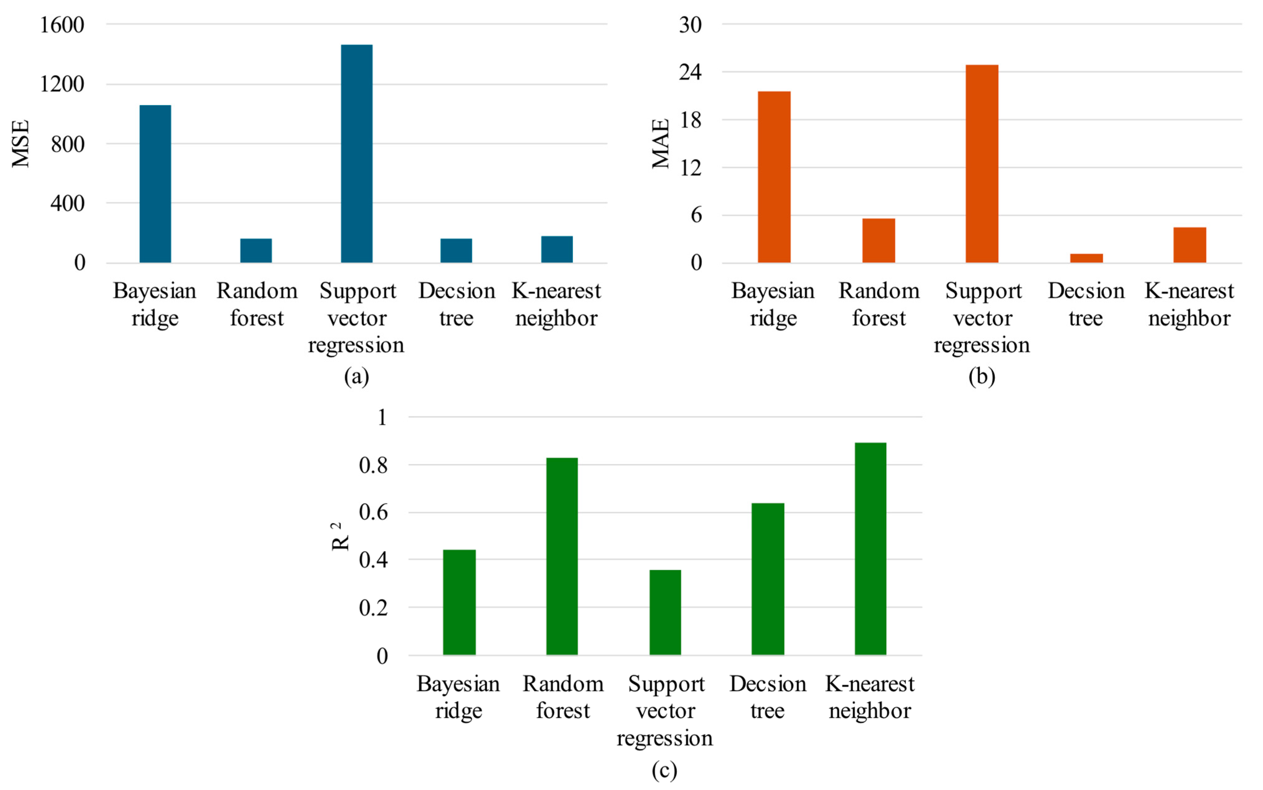
Multi-feature extraction from raw signalMSE1057.63159.11460.49158.24176.3
MAE21.655.5824.881.124.39
R 2 0.440.830.360.640.89
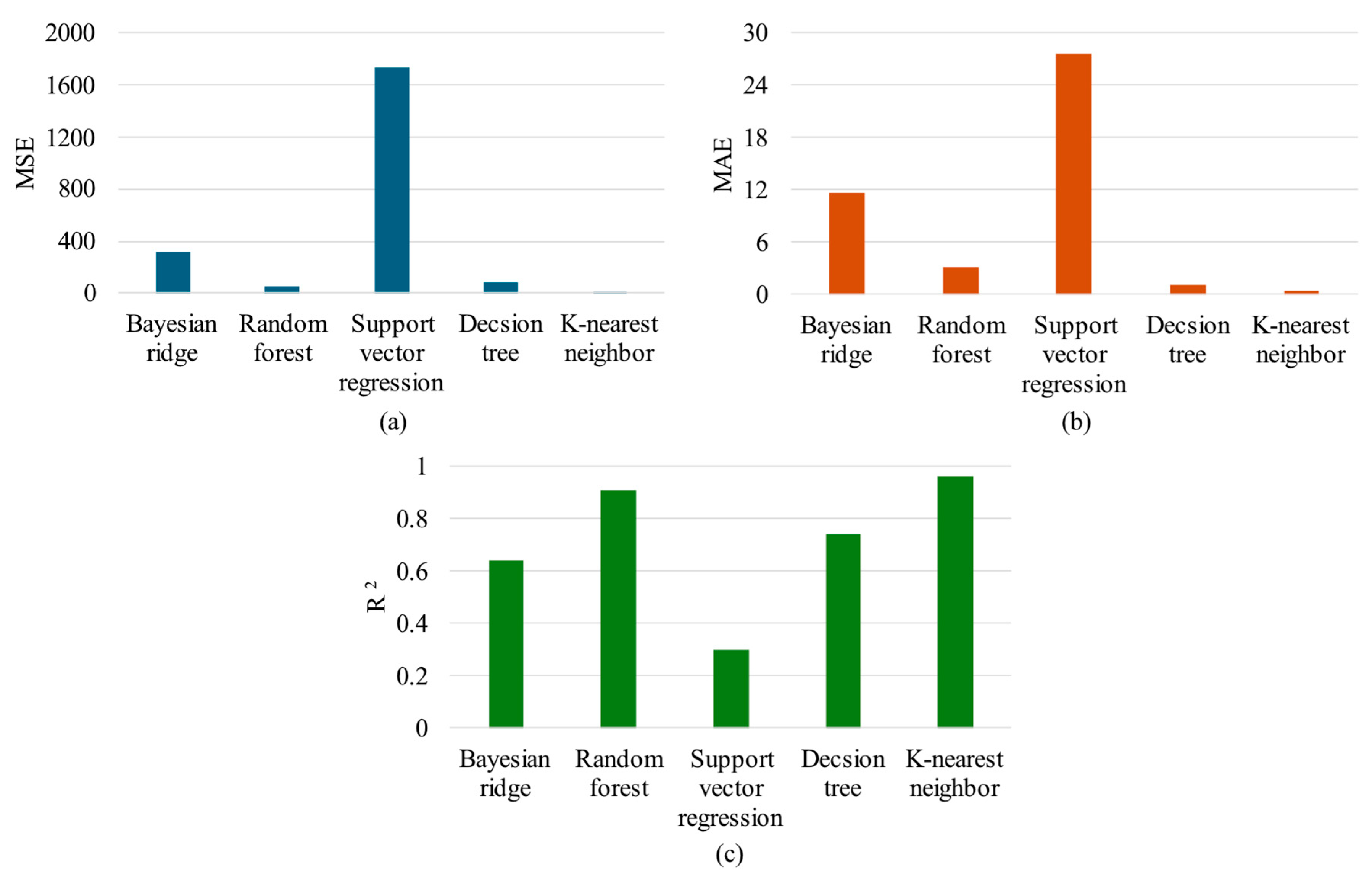
Multi-feature extraction from Hilbert transformMSE315.0252.511731.4379.1710.29
MAE11.653.227.581.10.5
R 2 0.640.910.30.740.96
Disclaimer/Publisher’s Note: The statements, opinions and data contained in all publications are solely those of the individual author(s) and contributor(s) and not of MDPI and/or the editor(s). MDPI and/or the editor(s) disclaim responsibility for any injury to people or property resulting from any ideas, methods, instructions or products referred to in the content.

