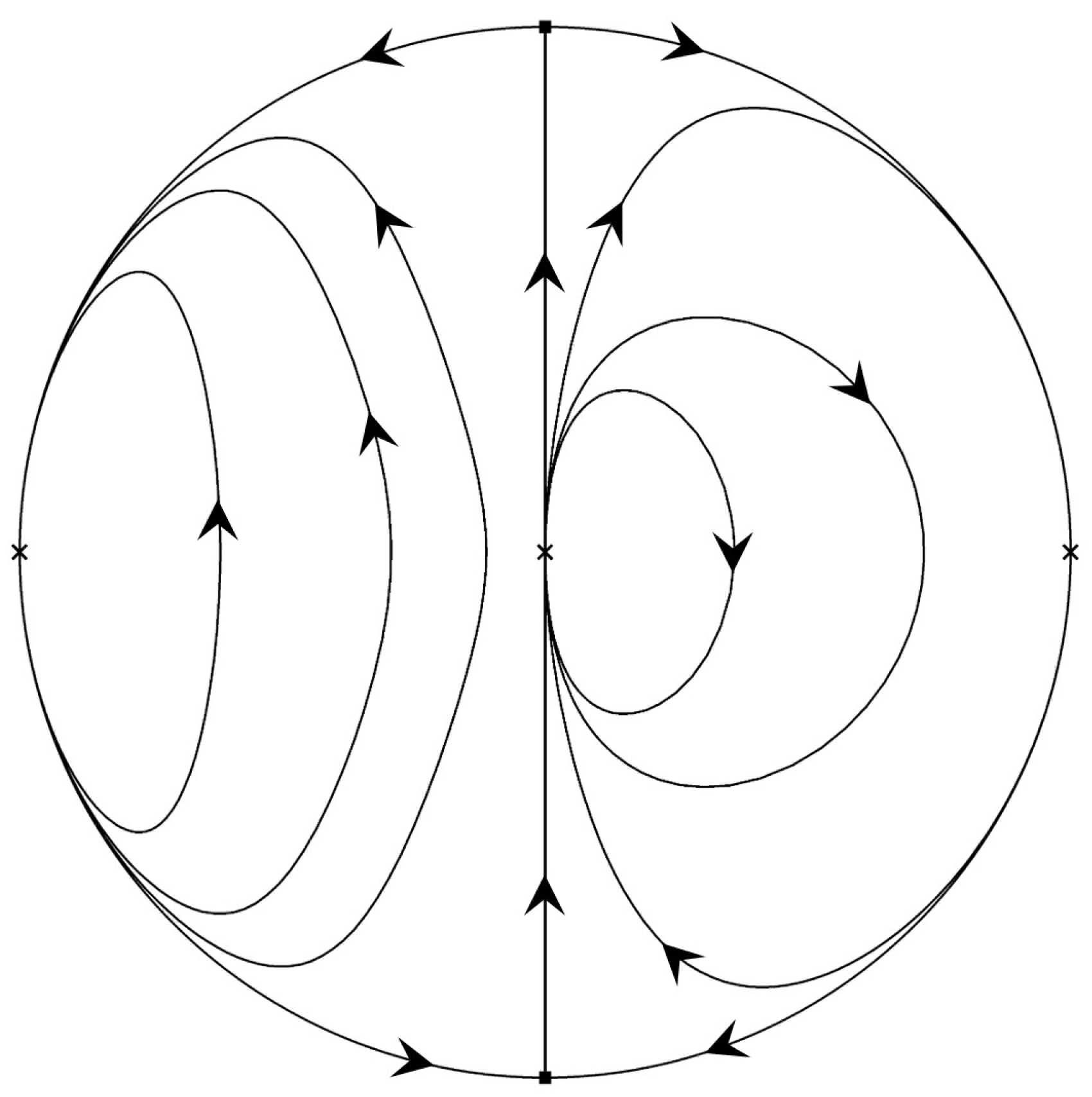
Article

The Global Dynamics of the Painlevé–Gambier Equations XVIII, XXI, and XXII

1
School of Sciences, Southwest Petroleum University, 610500 Chengdu, China
2
Departament de Matemàtiques, Universitat Autònoma de Barcelona, Bellaterra, 08193 Barcelona, Catalonia, Spain
*
Author to whom correspondence should be addressed.
These authors contributed equally to this work.
Mathematics 2025, 13(5), 756; https://doi.org/10.3390/math13050756
Submission received: 30 November 2024 / Revised: 2 January 2025 / Accepted: 23 February 2025 / Published: 25 February 2025

Abstract

:
In this paper, we describe the global dynamics of the Painlevé–Gambier equations numbered XVIII: x ( x ) 2 / ( 2 x ) 4 x 2 = 0 , XXI: x 3 ( x ) 2 / ( 4 x ) 3 x 2 , and XXII: x 3 ( x ) 2 / ( 4 x ) + 1 = 0 . We obtain three rational functions as their first integrals and classify their phase portraits in the Poincaré disc. The main reason for considering these three Painlevé–Gambier equations is due to the paper of Guha, P., et al., where the authors studied these three differential equations in order to illustrate a method to generate nonlocal constants of motion for a special class of nonlinear differential equations. Here, we want to complete their studies describing all of the dynamics of these equations. This demonstrates that the phase portraits of equations XVIII and XXI in the Poincaré disc are topologically equivalent.

1. Introduction

Some of the most studied differential systems are second-order ordinary differential equations (ODEs) x + F ( x , x ) = 0 , in particular those equivalent to conservation equations, x + g ( x ) = 0 , where the prime denotes the derivative with respect to the time t. By adding to a linear term of x , x + f ( x ) x + g ( x ) = 0 , we obtain the famous Liénard differential equation. In this paper, we consider a class of systems equivalent to second-order ordinary differential equations in which the quadratic term of x is considered,
x + f ( x ) ( x ) 2 + g ( x ) = 0 .
Such a study is motivated by a wide range of interests. In [1], the authors studied the following three types of the Painlevé–Gambier equations
XVIII 
x 1 2 x ( x ) 2 4 x 2 = 0 ,
XXI 
    x 3 4 x ( x ) 2 3 x 2 ,
XXII 
x 3 4 x ( x ) 2 + 1 = 0 .
They developed a method based on a generalization of the Sundman transformation in order to obtain new nonlocal first integrals of autonomous second-order ordinary differential equations.
The previous three differential equations are inside 50 second-order ordinary differential equations possessing a canonical form whose solutions have the Painlevé property developed by Painlevé, Gambier and their pupils. The results of [2] show that apart from 6 Painlevé-equations, the remaining 44 of the Painlevé–Gambier classification have solutions that can be expressed in terms of elementary functions. Ince studied many aspects of Painlevé–Gambier equations, for instance first integrals and analytical solutions (see the details in [3]). The authors of [4] used the generalized Sundman transformation method in order to construct other first integrals for some 50 differential equations classified by Painlevé and Gambier. For other results related to the Painlevé and Gambier, equations see [5,6].
The generalized Sundman transformation proposed by Akande et al. [7] is used to study the first integrals, symmetries, and solutions of equations using the Painlevé–Gambier method, such as trigonometric periodic solutions and periodic solutions in [1,7,8]. In [8], the authors calculated the explicit and exact general periodic solutions of the cubic Duffing equation and some Painlevé–Gambier equations. Kudryashov and Sinelshchikov studied connections between the Liénard equation and some equations of the Painlevé–Gambier type and obtained three new criteria for the integrability of the Liénard equation; see the details in [9]. Sinelshchikov, in [10], investigated nonlinear oscillators with quadratic damping, extending the Liénard equation, and demonstrated that nonlocal transformations preserved invariant curves, resulting in two integrable subfamilies associated with the Painlevé–Gambier classification, each with specific first integrals. Building on this, Ishchenko and Sinelshchikov, in 2023, further explored a family of nonlinear oscillators with quadratic damping and showed that nonlocal transformations preserved autonomous invariant curves. This facilitated the construction of two integrable subfamilies connected to the Painlevé–Gambier classification, along with their corresponding invariant curves and first integrals; see [11] for details.
The objective of this paper is to classify the phase portraits of Painlevé–Gambier equations XVIII, XXI, and XXII. These can be written as the following first-order ordinary differential equations
x = y , y = y 2 2 x + 4 x 2 .
x = y , y = 3 y 2 4 x + 3 x 2 .
x = y , y = 3 y 2 4 x 1 .
In the next theorem, we classify the phase portraits in the Poincaré disc of the differential systems (2)–(4). Generally speaking, the Poincaré disc is the closed unit disc centered at the origin of R 2 whose interior has been identified with R 2 and the boundary the circle is the infinity of R 2 . The polynomial differential equations in R 2 can be extended analytically to the Poincaré disc; in this way, we can study the dynamics of these differential systems near infinity; for more details, see Chapter 5 of [12] and see also [13].
Define the three functions
H 1 = H 1 ( x , y ) = y 2 4 x 3 x , H 2 = H 2 ( x , y ) = ( y 2 4 x 3 ) 2 x 3 , H 3 = H 3 ( x , y ) = ( y 2 4 x ) 2 x 3 .
Theorem 1.
In the Painlevé–Gambier classification, equation XVIII, (as well as XXI and XXII) has a rational first integral, denoted as H 1  (respectively, H 2 and H 3 ). Moreover, the phase portrait of the equations numbered XVIII and XXI in the Poincaré disc is shown in Figure 1a, and the phase portrait of the equation numbered XXII in the Poincaré disc is shown in Figure 1b.
Whethe the first integrals in the statement of Theorem 1 are first integrals can be easily checked using direct computations. The proof of Theorem 1 for systems XVIII and XXI is given in Section 2. The proof for system XXII is shown in Section 3.

2. The Painlevé–Gambier Equations XVIII and XXI

2.1. Finite Equilibrium Points

For the differential Equation (1), let
f ( x ) = a x , g ( x ) = b x 2
with two real parameters 0 < a < 1 and b > 0 , which is written as the first-order ordinary differential equations
x = y , y = a y 2 x + b x 2 .
It contains the Painlevé–Gambier equations numbered XVII and XXI if choosing a = 1 / 2 , b = 4 and a = 3 / 4 , b = 3 respectively. In order to obtain the phase portraits of the Painlevé–Gambier equations numbered XVII and XXI, we consider the differential system (5). For the change in time d s = d t / x , where t is the old time and s is the new time, we change the differential system to the polynomial form
x = x y , y = a y 2 + b x 3 ,
now the prime denotes the derivative with respect to the new time s. Further, using the change in variables x = ( a 1 / 3 / b 1 / 3 ) X and y = Y with 0 < a < 1 and b > 0 m we obtain a one-parameter differential system
x = x y , y = a ( y 2 + x 3 ) ,
here, we still use x and y instead of X and Y, respectively. Define the function
H = H ( x , y ) = 2 a x 3 + ( 2 a 3 ) y 2 ( 2 a 3 ) x 2 a .
We check that H is a first integral. Indeed, ( H / x ) ( x y ) + ( H / y ) ( a y 2 + a x 3 ) = 0 .
Clearly, the differential system (6) has a unique equilibrium point ( x , y ) = ( 0 , 0 ) , and its Jacobian is the zero matrix. In order to study the local phase portrait at the origin, we use blow ups as a tool to desingularize the equilibrium point; see for more details [14,15]. As the characteristic directions at the origin are ( 1 a ) x y 2 = 0 , it follows that x = 0 is a characteristic direction. Before allowing a vertical blow up, we apply the twist defined by x = x 1 y 1 and y = y 1 , and obtain
x 1 = x 1 y 1 + ( a 1 ) y 1 2 + a x 1 3 3 a x 1 2 y 1 + 3 a x 1 y 1 2 a y 1 3 , y 1 = a y 1 2 + a x 1 3 3 a x 1 2 y 1 + 3 a x 1 y 1 2 a y 1 3 .
Now, the characteristic directions at the origin are ( 1 a ) ( x 1 y 1 ) y 1 2 = 0 . So, x 1 = 0 is not a characteristic direction. Then, we perform a blow up defined by the change in variables x 1 = x 2 ,   y 1 = x 2 y 2 , along with the time rescaling d s = d τ / x 2 , and obtain
x 2 = a x 2 2 + x 2 y 2 3 a x 2 2 y 2 + ( a 1 ) x 2 y 2 2 + 3 a x 2 2 y 2 2 a x 2 2 y 2 3 , y 2 = a x 2 4 a x 2 y 2 + ( a 1 ) y 2 2 + 6 a x 2 y 2 2 ( a 1 ) y 2 3 4 a x 2 y 2 3 + a x 2 y 2 4 .
Now we compute the equilibrium points on the straight line x 2 = 0 . The computations show that there are two equilibrium points ( x 2 , y 2 ) = ( 0 , 0 ) and ( x 2 , y 2 ) = ( 0 , 1 ) .
Computing the Jacobian matrix evaluated at the equilibrium point ( 0 , 1 ) , we have that the equilibrium ( x 2 , y 2 ) = ( 0 , 1 ) is a hyperbolic node as the eigenvalues are 1 a and a. On the other hand, we check that the Jacobian matrix at ( 0 , 0 ) is nilpotent. Further, we use the change in variables defined by x 2 = y 3 and y 2 = a x 2 to transform the following
x 3 = y 3 + A ( x 3 , y 3 ) , y 3 = B ( x 3 , y 3 ) ,
where
A ( x 3 , y 3 ) = a ( a 1 ) x 3 2 4 a x 3 y 3 a 2 ( a 1 ) x 3 3 + 6 a 2 x 3 2 y 3 4 a 3 x 3 3 y 3 + a 4 x 3 4 y 3 , B ( x 3 , y 3 ) = a x 3 y 3 + a y 3 2 + a 2 ( a 1 ) x 3 2 y 3 3 a 2 x 3 y 3 2 + 3 a 3 x 3 2 y 3 2 a 4 x 3 3 y 3 2 .
Solving equation y 3 + A ( x 3 , y 3 ) = 0 , we obtain
y 3 = f ( x 3 ) = a ( a 1 ) x 3 2 ( a x 3 1 ) 3 .
Check that
F ( x 3 ) = B ( x 3 , f ( x 3 ) ) = a 2 ( 1 a ) x 3 3 + O ( x 3 4 ) , G ( x 3 ) = A ( x 3 , y 3 ) x 3 + B ( x 3 , y 3 ) y 3 | ( x 3 , f ( x 3 ) ) = a ( 2 a 1 ) x 3 .
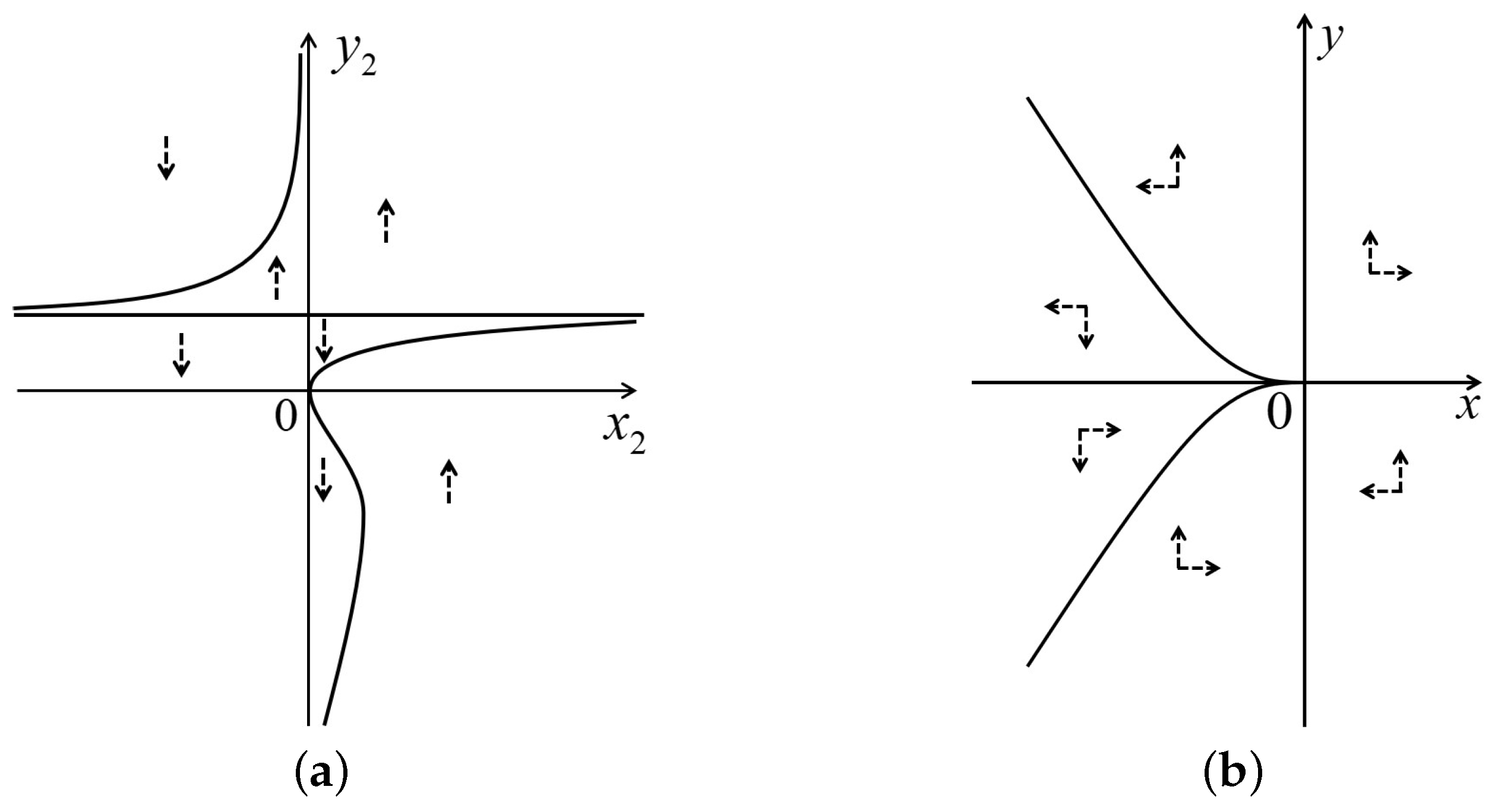
Then, there are two cases, a = 1 / 2 and a ( 0 , 1 / 2 ) ( 1 / 2 , 1 ) . From [12] (Theorem 3.5, p. 116), it follows that the equilibrium point ( x 2 , y 2 ) = ( 0 , 0 ) is a saddle in both cases. On the other hand, we see x 2 = 0 and y 2 = ( 1 a ) ( y 2 1 ) y 2 2 on the y 2 -axis. Note that the horizontal isocline H : ( y 2 1 ) ( a x 2 ( y 2 1 ) 3 + ( 1 a ) y 2 2 ) = 0 , from which we obtain y 2 = 1 and
x 2 = f ( y 2 ) = ( 1 a ) y 2 2 a ( y 2 1 ) 3 .
Consider the derivative of f
x 2 = f ( y 2 ) = ( 1 a ) y 2 ( y 2 + 2 ) a ( y 2 1 ) 4 ,
from which we obtain two zeros 0 and 2 . Moreover
f ( y 2 ) > 0 y 2 ( , 2 ) , f ( y 2 ) < 0 y 2 ( 2 , 0 ) , and f ( y 2 ) > 0 y 2 ( 0 , 1 ) ( 1 , + ) .
Further, f reaches a minimal value at y 2 = 0 and a maximal value at y 2 = 2 . Compute
lim y 2 f ( y 2 ) = 0 , f ( 2 ) = 4 ( 1 a ) 27 a , f ( 0 ) = 0 , lim y 2 1 f ( y 2 ) = + , lim y 2 1 + f ( y 2 ) = , lim y 2 + f ( y 2 ) = 0 .
Then, we see the graph of the horizontal isocline; see Figure 2a. Further, we obtain the vector field in the vertical direction for the differential system (7), as it is displayed in Figure 2a. Thus, we obtain the local phase portrait at the equilibrium points ( 0 , 0 ) and ( 0 , 1 ) ; see Figure 3a.
Going back to the differential system (6), we check that x = 0 and y = a y 2 on the y-axis. Then, combining the vector field in Figure 2b, we obtain one elliptic and one hyperbolic sector separated by two parabolic sectors at the origin; see Figure 3b.

2.2. Infinite Equilibrium Points

In order to study the dynamics near infinity for the differential system (6), we introduce the Poincaré compactification; see more details in [12,15]. First, in the local chart U 1 , the differential system becomes
u = a + ( a 1 ) u 2 v , v = u v 2 ,
and in the local chart, U 2 it becomes
u = ( 1 a ) u v a u 4 , v = a v 2 a u 3 v .
Clearly, we see that there are no infinite equilibrium points in the local chart U 1 , and the origin is an equilibrium point for the second differential system. Moreover, we observe that the Jacobian evaluated at the origin is the zero matrix. The characteristic directions at the origin are u v 2 = 0 . Then, we perform the twist defined by u = u 1 v 1 and v = v 1 and obtain the following
u 1 = ( 1 a ) u 1 v 1 v 1 2 a u 1 4 + 3 a u 1 3 v 1 3 a u 1 2 v 1 2 + a u 1 v 1 3 , v 1 = a v 1 2 a u 1 3 v 1 + 3 a u 1 2 v 1 2 3 a u 1 v 1 3 + a v 1 4 .
Now, the characteristic directions at the origin are v 1 2 ( u 1 v 1 ) = 0 . Thus, we perform the blow ups u 1 = u 2 ,   v 1 = u 2 v 2 to desingularize the origin and the time rescaling d s = d τ / u 2 , and obtain
u 2 = ( 1 a ) u 2 v 2 a u 2 3 u 2 v 2 2 + 3 a u 2 3 v 2 3 a u 2 3 v 2 2 + a u 2 3 v 2 3 , v 2 = v 2 2 + v 2 3 ,
where the prime presents the derivative with respect to the new time τ . Now, we compute the equilibrium points on the v 2 -axis and obtain two equilibrium points ( u 2 , v 2 ) = ( 0 , 0 ) and ( u 2 , v 2 ) = ( 0 , 1 ) . Clearly the linear part of the equilibrium point ( u 2 , v 2 ) = ( 0 , 0 ) is a zero matrix. On the other hand, the eigenvalues at ( u 2 , v 2 ) = ( 0 , 1 ) are 1 and a ; therefore, it is a hyperbolic saddle.
As the characteristic directions at the origin are ( 2 a ) u 2 v 2 2 = 0 , we use the twist defined by u 2 = u 3 v 3 , v 2 = v 3 before performing more blow ups, and obtain
u 3 = ( 1 a ) u 3 v 3 + ( a 2 ) v 3 2 a u 3 3 + 3 a u 3 2 v 3 ( 3 a + 1 ) u 3 v 3 2 + ( a + 2 ) v 3 3 + 3 a u 3 3 v 3 9 a u 3 2 v 3 2 + 9 a u 3 v 3 3 3 a v 3 4 3 a u 3 3 v 3 2 + 9 a u 3 2 v 3 3 9 a u 3 v 3 4 + 3 a v 3 5 + a u 3 3 v 3 3 3 a u 3 2 v 3 4 + 3 a u 3 v 3 5 a v 3 6 , v 3 = v 3 2 + v 3 3 .
Now, the characteristic directions at the origin are v 3 2 ( ( a 2 ) u 3 + 2 v 3 ) = 0 . Thus, we perform the blow ups with the change in variables u 3 = u 4 ,   v 3 = u 4 v 4 and the time rescaling d τ = d σ / u 4 2 , and obtain the following
u 4 = a u 4 2 + ( 1 a ) u 4 v 4 + 3 a u 4 2 v 4 + ( a 2 ) u 4 v 4 2 + 3 a u 4 3 v 4 ( 3 a + 1 ) u 4 2 v 4 2 9 a u 4 3 v 4 2 + ( a + 2 ) u 4 2 v 4 3 3 a u 4 4 v 4 2 + 9 a u 4 3 v 4 3 + 9 a u 4 4 v 4 3 3 a u 4 3 v 4 4 + a u 4 5 v 4 3 9 a u 4 4 v 4 4 3 a u 4 5 v 4 4 + 3 a u 4 4 v 4 5 + 3 a u 4 5 v 4 5 a u 4 5 v 4 6 , v 4 = a u 4 v 4 + ( a 2 ) v 4 2 3 a u 4 v 4 2 + ( 2 a ) v 4 3 3 a u 4 2 v 4 2 + ( 3 a + 2 ) u 4 v 4 3 + 9 a u 4 2 v 4 3 ( a + 2 ) u 4 v 4 4 + 3 a u 4 3 v 4 3 9 a u 4 2 v 4 4 9 a u 4 3 v 4 4 + 3 a u 4 2 v 4 5 a u 4 4 v 4 4 + 9 a u 4 3 v 4 5 + 3 a u 4 4 v 4 5 3 a u 4 3 v 4 6 3 a u 4 4 v 4 6 + a u 4 4 v 4 7 ,
where the prime denotes the derivative with respect to the new time σ . Considering the equilibrium points on the v 4 -axis, we obtain the two equilibrium points ( 0 , 0 ) and ( 0 , 1 ) . Moreover, we compute the Jacobian evaluated at ( 0 , 0 ) (respectively ( 0 , 1 ) ), and obtain a zero matrix (respectively, two eigenvalues −1 and 2 a ). It follows that the equilibrium point ( 0 , 1 ) is a hyperbolic saddle. For the local phase portrait at ( 0 , 0 ) , we need to perform more blow ups, but its characteristic directions at the origin are u 4 v 4 ( 2 a u 4 + ( 2 a 3 ) v 4 ) = 0 .
Similarly, we perforn the twist defined by u 4 = u 5 v 5 , v 4 = v 5 and see that the characteristic directions at the origin are v 5 ( v 5 u 5 ) ( 3 v 5 2 a u 5 ) = 0 because the twisted system is as follows
u 5 = a u 5 2 + ( 2 a + 1 ) u 5 v 5 3 v 5 2 + 3 a u 5 2 v 5 2 ( 4 a + 1 ) u 5 v 5 2 + 4 ( a + 1 ) v 5 3 + 3 a u 5 3 v 5 ( 15 a + 1 ) u 5 2 v 5 2 + 4 ( 6 a + 1 ) u 5 v 5 3 3 ( 4 a + 1 ) v 5 4 9 a u 5 3 v 5 2 + ( 37 a + 2 ) u 5 2 v 5 3 6 ( 8 a + 1 ) u 5 v 5 4 + 4 ( 5 a + 1 ) v 5 5 3 a u 5 4 v 5 2 + 24 a u 5 3 v 5 3 63 a u 5 2 v 5 4 + 66 a u 5 v 5 5 24 a v 5 6 + 9 a u 5 4 v 5 3 48 a u 5 3 v 5 4 + 93 a u 5 2 v 5 5 78 a u 5 v 5 6 + 24 a v 5 7 + a u 5 5 v 5 3 15 a u 5 4 v 5 4 + 59 a u 5 3 v 5 5 97 a u 5 2 v 5 6 + 72 a u 5 v 5 7 20 a v 5 8 3 a u 5 5 v 5 4 + 21 a u 5 4 v 5 5 57 a u 5 3 v 5 6 + 75 a u 5 2 v 5 7 48 a u 5 v 5 8 + 12 a v 5 9 + 3 a u 5 5 v 5 5 18 a u 5 4 v 5 6 + 42 a u 5 3 v 5 7 48 a u 5 2 v 5 8 + 27 a u 5 v 5 9 6 a v 5 10 a u 5 5 v 5 6 + 6 a u 5 4 v 5 7 14 a u 5 3 v 5 8 + 16 a u 5 2 v 5 9 9 a u 5 v 5 10 + 2 a v 5 11 , v 5 = a u 5 v 5 2 v 5 2 3 a u 5 v 5 2 + 2 ( a + 1 ) v 5 3 3 a u 5 2 v 5 2 + ( 9 a + 2 ) u 5 v 5 3 2 ( 3 a + 1 ) v 5 4 + 9 a u 5 2 v 5 3 ( 19 a + 2 ) u 5 v 5 4 + 2 ( 5 a + 1 ) v 5 5 + 3 a u 5 3 v 5 3 18 a u 5 2 v 5 4 + 27 a u 5 v 5 5 12 a v 5 6 9 a u 5 3 v 5 4 + 30 a u 5 2 v 5 5 33 a u 5 v 5 6 + 12 a v 5 7 a u 5 4 v 5 4 + 13 a u 5 3 v 5 5 33 a u 5 2 v 5 6 + 31 a u 5 v 5 7 10 a v 5 8 + 3 a u 5 4 v 5 5 15 a u 5 3 v 5 6 + 27 a u 5 2 v 5 7 21 a u 5 v 5 8 + 6 a v 5 9 3 a u 5 4 v 5 6 + 12 a u 5 3 v 5 7 18 a u 5 2 v 5 8 + 12 a u 5 v 5 9 3 a v 5 10 + a u 5 4 v 5 7 4 a u 5 3 v 5 8 + 6 a u 5 2 v 5 9 4 a u 5 v 5 10 + a v 5 11 .
Furthermore, we perform the change in variables u 5 = u 6 ,   v 5 = u 6 v 6 and the rescaling time d σ = ς / u 6 , and obtain the following
u 6 = a u 6 + ( 2 a + 1 ) u 6 v 6 + 3 a u 6 2 v 6 3 u 6 v 6 2 + 3 a u 6 3 v 6 2 ( 4 a + 1 ) u 6 2 v 6 2 ( 15 a + 1 ) u 6 3 v 6 2 + 4 ( a + 1 ) u 6 2 v 6 3 9 a u 6 4 v 6 2 + 4 ( 6 a + 1 ) u 6 3 v 6 3 3 a u 6 5 v 6 2 + ( 37 a + 2 ) u 6 4 v 6 3 3 ( 4 a + 1 ) u 6 3 v 6 4 + 24 a u 6 5 v 6 3 6 ( 8 a + 1 ) u 6 4 v 6 4 + 9 a u 6 6 v 6 3 63 a u 6 5 v 6 4 + 4 ( 5 a + 1 ) u 6 4 v 6 5 + a u 6 7 v 6 3 48 a u 6 6 v 6 4 + 66 a u 6 5 v 6 5 15 a u 6 7 v 6 4 + 93 a u 6 6 v 6 5 24 a u 6 5 v 6 6 3 a u 6 8 v 6 4 + 59 a u 6 7 v 6 5 78 a u 6 6 v 6 6 + 21 a u 6 8 v 6 5 97 a u 6 7 v 6 6 + 24 a u 6 6 v 6 7 + 3 a u 6 9 v 6 5 57 a u 6 8 v 6 6 + 72 a u 6 7 v 6 7 18 a u 6 9 v 6 6 + 75 a u 6 8 v 6 7 20 a u 6 7 v 6 8 a u 6 10 v 6 6 + 42 a u 6 9 v 6 7 48 a u 6 8 v 6 8 + 6 a u 6 10 v 6 7 48 a u 6 9 v 6 8 + 12 a u 6 8 v 6 9 14 a u 6 10 v 6 8 + 27 a u 6 9 v 6 9 + 16 a u 6 10 v 6 9 6 a u 6 9 v 6 10 9 a u 6 10 v 6 10 + 2 a u 6 10 v 6 11 , v 6 = 2 a v 6 ( 2 a + 3 ) v 6 2 6 a u 6 v 6 2 + 3 v 6 3 6 a u 6 2 v 6 2 + 2 ( 5 a + 2 ) u 6 v 6 3 + 3 ( 8 a + 1 ) u 6 2 v 6 3 4 ( a + 1 ) u 6 v 6 4 + 18 a u 6 3 v 6 3 6 ( 5 a + 1 ) u 6 2 v 6 4 + 6 a u 6 4 v 6 3 4 ( 14 a + 1 ) u 6 3 v 6 4 + 3 ( 4 a + 1 ) u 6 2 v 6 5 42 a u 6 4 v 6 4 + 2 ( 29 a + 4 ) u 6 3 v 6 5 18 a u 6 5 v 6 4 + 90 a u 6 4 v 6 5 4 ( 5 a + 1 u 6 3 ) v 6 6 2 a u 6 6 v 6 4 + 78 a u 6 5 v 6 5 78 a u 6 4 v 6 6 + 28 a u 6 6 v 6 5 126 a u 6 5 v 6 6 + 24 a u 6 4 v 6 7 + 6 a u 6 7 v 6 5 92 a u 6 6 v 6 6 + 90 a u 6 5 v 6 7 36 a u 6 7 v 6 6 + 128 a u 6 6 v 6 7 24 a u 6 5 v 6 8 6 a u 6 8 v 6 6 + 84 a u 6 7 v 6 7 82 a u 6 6 v 6 8 + 30 a u 6 8 v 6 7 96 a u 6 7 v 6 8 + 20 a u 6 6 v 6 9 + 2 a u 6 9 v 6 7 60 a u 6 8 v 6 8 + 54 a u 6 7 v 6 9 10 a u 6 9 v 6 8 + 60 a u 6 8 v 6 9 12 a u 6 7 v 6 10 + 20 a u 6 9 v 6 9 30 a u 6 8 v 6 10 20 a u 6 9 v 6 10 + 6 a u 6 8 v 6 11 + 10 a u 6 9 v 6 11 2 a u 6 9 v 6 12 ,
where the prime shows the derivative with respect to the new time ς . Considering the equilibrium points on the v 6 -axis, we see that there are three equilibrium points, ( 0 , 0 ) , ( 0 , 2 a / 3 ) , and ( 0 , 1 ) . Computing the Jacobian matrix at each equilibrium point, we see that the eigenvalues are 2 a and a at ( 0 , 0 ) , a / 3 and 2 a ( 2 a 3 ) / 3 at ( 0 , 2 a / 3 ) , and 3 2 a and a 2 at ( 0 , 1 ) . It follows that ( 0 , 0 ) and ( 0 , 1 ) are two saddles and ( 0 , 2 a / 3 ) is a stable node as 0 < a < 1 . Note that u 6 | u 6 = 0 = 0 and v 6 | u 6 = 0 = v 6 ( v 6 1 ) ( 2 a 3 v 6 ) . Then, the v 6 -axis is an invariant line. Similarly, we see u 6 | v 6 = 0 = a u 6 and v 6 | v 6 = 0 = 0 , and u 6 | v 6 = 1 = ( a 2 ) u 6 ( u 6 1 ) and v 6 | v 6 = 1 = 0 , implying that the u 6 -axis and the line v 6 = 1 are invariant. Thus, we obtain the local phase portrait at the three equilibrium points; see Figure 4a.
Returning to the differential system (10), we see
u 4 | u 4 = 0 = 0 , v 4 | u 4 = 0 = ( 2 a ) v 4 2 ( v 4 1 ) , u 4 | v 4 = 0 = a u 4 2 , v 4 | v 4 = 0 = 0 , u 4 | v 4 = 1 = u 4 ( u 4 1 ) , v 4 | v 4 = 1 = 0 .
Thus, the u 4 -axis, v 4 -axis, and v 4 = 1 are invariant. Further, we obtain the local phase portrait at the two equilibrium points ( 0 , 0 ) and ( 0 , 1 ) ; see Figure 4b. As for the differential system (9), we similarly have
u 2 | u 2 = 0 = 0 , v 2 | u 2 = 0 = v 2 2 ( v 2 1 ) , u 2 | v 2 = 0 = a u 2 3 , v 2 | v 2 = 0 = 0 , u 2 | v 2 = 1 = a u 2 , v 2 | v 2 = 1 = 0 .
Thus, the u 2 -axis, the v 2 -axis, and v 2 = 1 are also invariant, and the local phase portrait is given in Figure 4c. Eventually, we obtain the local phase portrait at the origin of the local chart U 2 (see Figure 4d), where the u-axis and v-axis are invariant because u | u = 0 = 0 , v | u = 0 = a v 2 < 0 and u | v = 0 = a u 4 < 0 , v | v = 0 = 0 .

2.3. Phase Portraits of Painlevé–Gambier Equations XVIII and XXI

From the two Figure 3b and Figure 4d, we obtain the phase portrait of the differential system (6); see Figure 5. Recalling the time rescaling d s = d t / x and going back to the differential system (5) containing the Painlevé–Gambier equations XVIII and XXI, the phase portrait is shown in Figure 1a.

3. The Painlevé–Gambier Equation XXII

3.1. Finite Equilibrium Points

We end with the study of the Painlevé–Gambier equation XXII. With the time rescaling d s = d t / ( 4 x ) , it becomes a polynomial differential system
x = 4 x y , y = 3 y 2 4 x ,
where the prime denotes the derivative with respect to the new time s. We check that the function
H = ( y 2 4 x ) 2 x 3
is a first integral for the differential system (12). In order to obtain the phase portrait in the Poincaré disc of the differential system (12), we see that the origin is a unique equilibrium point. Furthermore, we have that its linear part is nilpotent. Through completing the change in variables x = y 1 and y = 4 x 1 , it becomes the following
x 1 = y 1 12 x 1 2 , y 1 = 16 x 1 y 1 .
Let A ( x 1 ) = 12 x 1 2 and B ( x 1 , y 1 ) = 16 x 1 y 1 . Then, from equation y 1 + A ( x 1 ) = 0 , we see
y 1 = f ( x 1 ) = 12 x 1 2 .
On the other hand
F ( x 1 ) = B ( x 1 , f ( x 1 ) ) = 192 x 1 3 , G ( x 1 ) = A ( x 1 , y 1 ) x 1 + B ( x 1 , y 1 ) y 1 | ( x 1 , f ( x 1 ) ) = 40 x 1 .
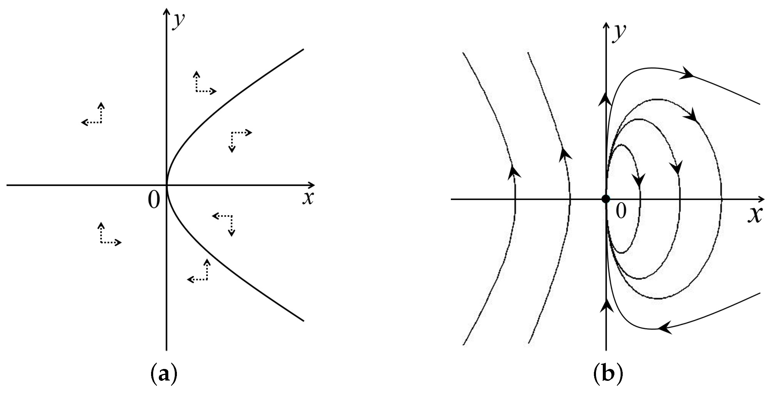
From [12] (Theorem 3.5, p.116), the phase portrait of the origin ( x 1 , y 1 ) = ( 0 , 0 ) consists of one hyperbolic and one elliptic sector. Note that x | x = 0 = 0 and y | x = 0 = 3 y 2 , implying that the y-axis is invariant. Together with the horizontal isocline x = 3 y 2 / 4 from the second equation in (12), we see the vector field, as it is shown in Figure 6a. Thus, we obtain the local phase portrait at the origin for the differential system (12); see Figure 6b.

3.2. Infinite Equilibrium Points

Now, we study the local phase portraits at the infinite equilibria. First, in the local chart U 1 , the differential system (12) becomes
u = u 2 4 v , v = 4 u v ,
and in the local chart U 2 it becomes
u = u + 4 u 2 v , v = 3 v + 4 u v 2 .
Clearly, the origin of the local chart U 1 is the unique equilibrium point on the u-axis for the first differential system and the origin the local chart U 2 is an equilibrium point for the second differential system.
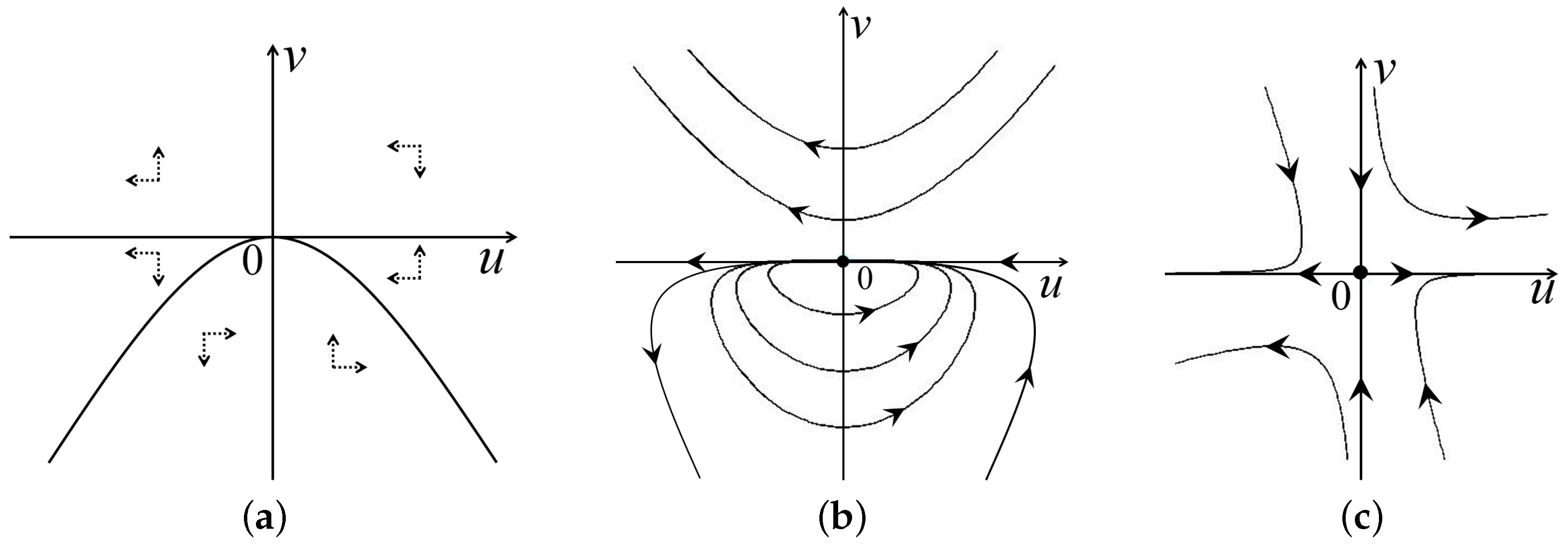
On the other hand, we see that the linear part of the differential system (13) is nilpotent. As it is discussed for the origin at the differential system (12), we similarly obtain that the phase portrait of the origin for the local chart U 1 consists of one hyperbolic and one elliptic sector. Noting the horizontal isocline v = u 2 / 4 by (13), we have that the vector field are displayed in Figure 7a. Since u | v = 0 = u 2 and v | v = 0 = 0 we see that the u-axis is invariant. Thus we obtain the local phase portrait at the origin for the differential system (13); see Figure 7b.
Evaluated at the origin of the local chart U 2 , the eigenvalues are 3 and 1, implying that it is a saddle. On the other hand, u | u = 0 = 0 and v | u = 0 = 3 v , and u | v = 0 = u and v | v = 0 = 0 , implying that the u-axis and v-axis are invariant. Its local phase portrait is displayed in Figure 7c.

3.3. Phase Portraits of Painlevé–Gambier Equation XXII

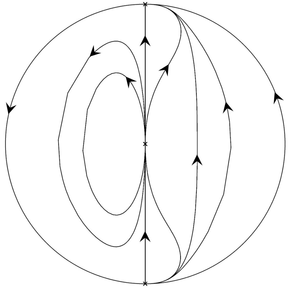
Combing the three Figure 6b and Figure 7b,c, we obtain the phase portrait of the differential system (12); see Figure 8. Recalling the time rescaling d s = d t / ( 4 x ) and going back to the Painlevé–Gambier equation XXII, we obtain the phase portrait, as it is shown in Figure 1b.

Author Contributions

Conceptualization, J.L. (Jie Li) and J.L. (Jaume Llibre); methodology, J.L. (Jie Li) and J.L. (Jaume Llibre); validation, J.L. (Jie Li) and J.L. (Jaume Llibre); formal analysis, J.L. (Jie Li) and J.L. (Jaume Llibre); investigation, J.L. (Jie Li) and J.L. (Jaume Llibre); resources, J.L. (Jie Li) and J.L. (Jaume Llibre); writing—original draft preparation, J.L. (Jie Li) and J.L. (Jaume Llibre); writing—review and editing, J.L. (Jie Li) and J.L. (Jaume Llibre); visualization, J.L. (Jie Li) and J.L. (Jaume Llibre). All authors have read and agreed to the published version of the manuscript.

Funding

The first author is partially supported by the natural science starting project of SWPU (No. 2023QHZ016) and NSFC #1240012853. The second author is partially supported by the Agencia Estatal de Investigación grant PID2022-136613NB-100, the H2020 European Research Council grant MSCA-RISE-2017-777911, AGAUR (Generalitat de Catalunya) grant 2021SGR00113, and by the Real Acadèmia de Ciències i Arts de Barcelona.

Data Availability Statement

The original contributions presented in this study are included in the article. Further inquiries can be directed to the corresponding author.

Conflicts of Interest

The authors declare no conflicts of interest.

References

  1. Guha, P.; Choudhury, A.G.; Khanra, B.; Leach, P.G.L. Nonlocal Constants of Motions of Equations of Painlevé-Gambier Type and Generalized Sundman Transformation. Russ. J. Nonlinear Dyn. 2022, 18, 103–118. [Google Scholar] [CrossRef]
  2. Gromak, V.A.; Lukashevich, N.A. The Analytic Solutions of the Painlevé Equations. Universitetskoye: Minsk, Belarus, 1990. (In Russian) [Google Scholar]
  3. Ince, E.L. Differential equations in the complex domain. In Ordinary Differential Equations; Dover: New York, NY, USA, 1956; pp. 317–355. [Google Scholar]
  4. Guha, P.; Khanra, B.; Choudhury, A.G. On generalized Sundman transformation method, first integrals, symmetries and solutions of equations of Painlevé-Gambier type. Nonlinear Anal. Theory Methods Appl. 2010, 72, 3247–3257. [Google Scholar] [CrossRef]
  5. Conte, R.; Musette, M.; Grundland, A.M. Bäcklund transformation of partial differential equations from the Painlevé-Gambier classification. II. Tzitzéica equation. J. Math. Phys. 1999, 40, 2092–2106. [Google Scholar] [CrossRef]
  6. Musette, M.; Conte, R. Backlund transformation of partial differential equations from the Painlevé-Gambier classification, I. Kaup-Kupershmidt equation. J. Math. Phys. 1998, 39, 5617–5630. [Google Scholar] [CrossRef]
  7. Akande, J.; Kêgnidé Adjaï, D.K.; Monsia, M.D. Theory of exact trigonometric periodic solutions to quadratic Liénard type equations. J. Math. Stat. 2018, 14, 232–240. [Google Scholar] [CrossRef]
  8. Kêgnidé Adjaï, D.K.; Koudahoun, L.H.; Akande, J.; Kpomahou, Y.J.F.; Monsia, M.D. Solutions of the Duffing and Painlevé-Gambier Equations by Generalized Sundman Transformation. J. Math. Stat. 2018, 14, 241–252. [Google Scholar] [CrossRef]
  9. Kudryashov, N.A.; Sinelshchikov, D.I. On connections of the Liénard equation with some equations of Painlevé-Gambier type. J. Math. Anal. Appl. 2017, 449, 1570–1580. [Google Scholar] [CrossRef]
  10. Sinelshchikov, D.I. Nonlocal deformations of autonomous invariant curves for Liénard equations with quadratic damping. Chaos Solitons Fractals 2021, 152, 111412. [Google Scholar] [CrossRef]
  11. Ishchenko, A.R.; Sinelshchikov, D.I. On an integrable family of oscillators with linear and quadratic damping. Chaos Solitons Fractals 2023, 176, 114082. [Google Scholar] [CrossRef]
  12. Dumortier, F.; Llibre, J.; Artés, J.C. Qualitative Theory of Planar Differential Systems; Springer: New York, NY, USA, 2006. [Google Scholar]
  13. Diz-Pita, E.; Llibre, J.; Otero-Espinar, M.V. Phase portraits of a family of Kolmogorov systems with infinitely many singular points at infinity. Commun. Nonlinear Sci. Numer. Simul. 2022, 104, 106038. [Google Scholar] [CrossRef]
  14. Andronov, A.A.; Leontovich, E.A.; Gordon, I.I.; Muier, A.G. Qualitative Theory of Second-Order Dynamic Systems; John Wiley & Sons: New York, NY, USA; Toronto, ON, Canada, 1973. [Google Scholar]
  15. Zhang, Z.; Ding, T.; Huang, W.; Dong, Z. Critical Points at Infinity. In Qualitative Theory of Differential Equations; American Mathematical Society: Providence, RI, USA, 1992; pp. 321–331. [Google Scholar]
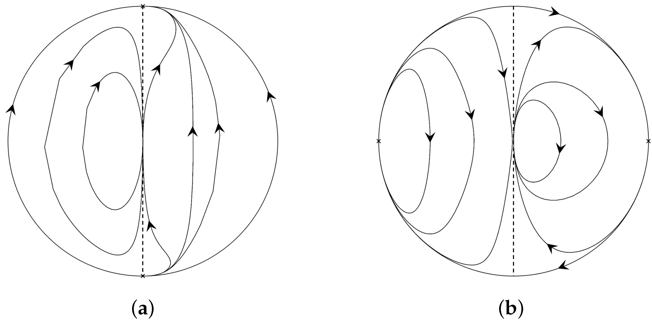
Figure 1. Figure (a) is the phase portrait of differential equations XVIII and XXI, and Figure (b) is the phase portrait of the differential equation XXII. The dashed straight line in both figures denotes the straight line x = 0 , where these differential systems are not defined.
Mathematics 13 00756 g001
Figure 2. The horizontal isocline is displayed in Figure (a) for the differential system (7). The vector field is displayed in Figure (b) for the differential system (6).
Mathematics 13 00756 g002
Figure 3. Figure (a) is the local phase portrait at the origin for the differential system (7), and Figure (b) is the local phase portrait at the origin for the differential system (6).
Mathematics 13 00756 g003
Figure 4. (a) The local phase portrait at the three equilibrium points ( 0 ,   0 ) ,   ( 0 ,   2 a / 3 ) , and ( 0 ,   1 ) for the differential system (11). (b) The local phase portrait at ( 0 ,   0 and ( 0 ,   1 ) for the differential system (10). (c) The local phase portrait at ( 0 ,   0 and ( 0 ,   1 ) for the differential system (9). Finally, the local phase portrait of the differential system (8) is shown in Figure (d).
Mathematics 13 00756 g004
Figure 5. The phase portrait of the differential system (6).
Mathematics 13 00756 g005
Figure 6. Figure (a) is the vector field of the differential system (12), and Figure (b) is the local phase portrait at the origin for the differential system (12).
Mathematics 13 00756 g006
Figure 7. Figure (a) is the vector field of the differential system (13). Figure (b) is the local phase portrait at the origin for the differential system (13). Figure (c) is the local phase portrait at the origin for the differential system (14).
Mathematics 13 00756 g007
Figure 8. The phase portrait of the differential system (12).
Mathematics 13 00756 g008
Disclaimer/Publisher’s Note: The statements, opinions and data contained in all publications are solely those of the individual author(s) and contributor(s) and not of MDPI and/or the editor(s). MDPI and/or the editor(s) disclaim responsibility for any injury to people or property resulting from any ideas, methods, instructions or products referred to in the content.