Detection of a Spatial Source Term Within a Multi-Dimensional, Multi-Term Time-Space Fractional Diffusion Equation

Abstract

The main objective of this study was to identify the undetermined source term (ST) in a fractional space-time scattering equation with multiple terms, using data obtained from the most recent observations. To address this complex problem, we reformulated the equation by adopting a regularization-based optimization approach. This methodology not only makes it possible to determine the existence of a single minimum solution, but also to assess its stability. In the numerical context, we estimate and approach the function (ST) by applying the Levenberg–Marquardt regularization method, a powerful tool for solving inverse problems. In order to demonstrate the effectiveness of the proposed approach, we performed numerical simulations in one-dimensional and two-dimensional scenarios. These simulations illustrate our method’s ability to process complex data and provide accurate and stable solutions. Through this extended approach, we aimed to discover the single source term in a multi-term space-time fractional scattering equation, ensuring robust and reliable results, supported by the most recent observational data.

1. Introduction

The inverse problem for differential equations is an important field of study with a wide range of applications in various practical sciences. Over the past few decades, many theoretical and computational methods have been developed to solve and evaluate different types of partial differential problem. More precisely, the reconstruction of the source term (ST) in fractional differential equations (FCEs) represents a particularly complex mathematical and computational problem. This task consists of determining an unknown input source or function based on the observed data of the solution of a fractional differential equation [1,2].

This complex problem has important implications and applications in several scientific and technical fields. For example, in medical imaging and biomathematics, the inverse problem helps develop models to better understand biological processes and improve imaging techniques. In environmental science and geophysics, it is used to model and predict natural phenomena, such as groundwater flow and seismic activities [3,4].

In the field of electrochemistry, solving the inverse problem for EDFs helps understand and optimize electrochemical processes [5,6]. Similarly, in economics and finance, these methods are applied to model financial markets and forecast economic trends [7,8].

In general, the ability to reconstruct the source term in fractional differential equations is crucial for advancing knowledge and technology in these varied fields. The Levenberg–Marquardt regularization method is one of the techniques used to obtain precise and stable solutions to these complex inverse problems, highlighting the continued importance of developing robust computational approaches [9,10,11].

For background, the inverse problem for differential equations has wide applications in a variety of practical sciences, and multiple theoretical and computational approaches to solving and evaluating various types of partial differential problems have been developed in the literature during the last few decades [12,13]. Reconstructing the ST in fractional differential equations (FDEs) is a challenging mathematical and computational problem that involves determining an unknown source or input function based on observed data of the solution to a fractional differential equation. This problem has several applications across various scientific and engineering fields, where it is necessary to infer or estimate the source or driving function behind observed phenomena. Here are some applications of the inverse source problem for FDEs: medical imaging and biomathematics, environmental science and geophysics, electrochemistry, economics and finance.

For example, this inverse source problem has been studied in various aspects on a large scale. X. Yan et al. [14] consider a non-stationary iterative Tikhonov regularization method combined with a finite-dimensional approximation to find the space-dependent ST in a multi-dimensional time-fractional diffusion-wave equation from a part of noisy boundary data. T. Wei et al. [15] proposed a conjugate gradient algorithm to identify the time-dependent ST in a multi-dimensional time-fractional diffusion equation from boundary Cauchy data. In [16], Y. S. Li et al. study the identification of a time-dependent ST in a time-space fractional diffusion-wave equation by utilizing additional measurements of the solute concentration distribution either at a point along the boundary or within the solution domain. M. Chang [17] proposed the Landweber iterative regularization method to reconstruct the ST in a multi-term time-fractional diffusion equation. The task is to extract this equation from noisy final data within a general bounded domain. In the next section, we consider the following problem:

$$\left\{\begin{array}{ccccc}\hfill {\displaystyle \sum _{i=1}^p{q}_i{\partial }_t^{{\alpha }_i}y+{(-\Delta )}^{\frac{s}{2}}y}& =& f\left(t\right)g\left(x\right)\hfill & \mathrm{in}& \Omega \times (0,T],\hfill \\ \hfill y& =& 0\hfill & \mathrm{in}& {\mathbb{R}}^d\setminus \Omega \times (0,T],\hfill \\ \hfill y(·,0)& =& y_0\hfill & \mathrm{in}& \Omega .\hfill \end{array}\right.$$

(1)

where:

• $\Omega \subset {\mathbb{R}}^d(d=1,2)$ is an open set with bounded limits;
• For a given positive integer p, let $q_i$ and $\alpha =\{{\alpha }_i:i=1,2,\cdots ,p\}$ be positive constants such that $0<{\alpha }_p<\cdots <{\alpha }_1;$
• ${\partial }_t^{{\alpha }_i}y$ is the Djrbashian–Caputo fractional derivative in time of order ${\alpha }_i\in (0,1)$ defined by:

  $${\partial }_t^{{\alpha }_i}y={\displaystyle \frac{1}{\Gamma (1-{\alpha }_i)}}{\int }_0^t{(t-s)}^{-{\alpha }_i}{y}^{\prime }\left(s\right)ds$$

  (2)

  where the function $\Gamma$ is defined by ${\displaystyle \Gamma \left(z\right)={\int }_0^{\infty }{s}^{z-1}\exp (-s)ds}$;
• The fractional operator ${\displaystyle {(-\Delta )}^{\frac{s}{2}}}$ is defined in the standard manner and can be expressed using the Laplace operator. This representation utilizes the spectral decomposition for $s\in (1,2)$.

For the Laplacian operator $-\Delta$, we denote the eigenvectors and eigenvalues $\{{\psi }_k,{\lambda }_k\}$ such that

$$\left\{\begin{array}{cc}-\Delta {\psi }_k& ={\lambda }_k{\psi }_k\mathrm{in}\Omega ,\\ {\psi }_k& =0\mathrm{in}\partial \Omega .\end{array}\right.$$

We select the following:

$${\mathcal{G}}_{\theta }=\left\{\begin{array}{c}g=\sum _{i=1}^{\infty }{b}_i{\psi }_i,b_n=(g,{\psi }_i)\left|\sum _{i=1}^{\infty }\right|b_n{|}^2{\left|{\lambda }_i\right|}^{\theta }<\infty ,\theta =\max (0,s)\end{array}\right\}.$$

Hence, we can write

$${(-\Delta )}^{{\displaystyle \frac{s}{2}}}=\sum _{i=1}^{\infty }{b}_i{\lambda }_i^{{\displaystyle \frac{s}{2}}}{\psi }_i.$$

The eigenvalues ${\lambda }_i$ and eigenfunctions ${\psi }_i$ are determined by the boundary conditions and geometry of the domain $\Omega$. In a rectangular domain, for example, they can be analytically derived using the separation of variables method.

For intricate geometries, numerical techniques such as finite element analysis and spectral methods are frequently employed to compute eigenfunctions and eigenvalues. The spectral decomposition of the Laplace operator serves as a fundamental concept in the analysis of partial differential equations, with significant applications across disciplines such as physics, engineering, and applied mathematics. This approach provides a robust framework for addressing the boundary value and eigenvalue problems, offering valuable insights into the behavior of differential equation solutions across diverse domains [18].

This paper aims to incorporate space-dependent ST into a multi-term time-fractional diffusion equation. The primary objective is to reconstruct the spatially varying source term $g\left(x\right)\in L^2(\Omega )$ based on the final observation data $\mathcal{Z}\left(x\right)\in L^2(\Omega )$ in both the one- and two-dimensional cases. The inverse problem associated with the multi-term time-space fractional diffusion equation was addressed computationally using the Levenberg–Marquardt regularization technique.

Existing studies like [19,20] focus on recovering an unknown space-dependent source term in fractional diffusion equations. This study extends the analysis to a multi-term fractional scattering equation in space-time, thus providing a more generalized structure. A key contribution of this work is the application of a regularization-based optimization framework, ensuring the stability and uniqueness of the reconstructed source term. The integration of the Levenberg–Marquardt regularization method further improves numerical accuracy, making it a robust approach for solving inverse problems in fractional scattering. Unlike previous methodologies that rely on single-term formulations or limited dimensional approximations, our model is able to handle complex multi-term dynamics in both one-dimensional and two-dimensional domains. The numerical experiments confirm the effectiveness of the proposed method, which demonstrates a high accuracy and stability, even in the presence of noisy data. These results significantly improve the applicability of fractional scattering models in areas such as biomedical imaging, environmental modeling, and thermal conduction, where the accurate identification of the source term is crucial. Compared to existing studies such as [21,22], our approach offers a more comprehensive and flexible framework, effectively addressing limitations in stability and computational feasibility.

The organizational structure of the paper is outlined as follows:

This research paper is structured into six sections. The investigation begins with Section 1, which sets the groundwork by providing a contextual framework and a comprehensive review of the research topic. Next, Section 2 explores the fundamental aspects and uniqueness properties of the solutions of the direct problem related to a multi-term time-space fractional diffusion equation. Section 3 addresses the inverse problem of determining the ST using the well-established Tikhonov method. This section formulates the problem in an optimization framework, looking for its minimizer while establishing the existence, stability, and uniqueness of the solution. Section 4, devoted to the methodology, develops an identification approach based on the Levenberg–Marquardt regularization method to solve the inverse problem of the source. The findings of this investigation are presented and analyzed in depth in Section 5, where the practical implications and the effectiveness of the proposed approach are explored. Finally, Section 6 synthesizes the key findings and presents the main conclusions drawn from this research.

The paper follows a well-defined structure with numbered sections and subsections for clarity. Mathematical formulations are presented using numbered equations and well-defined theorems. The section on regularization and the stability analysis contains structured demonstrations, while the section on the identification approach details the computational framework. The numerical testing section is divided into one-dimensional and two-dimensional cases, with annotated tables and figures to illustrate the results. The article concludes with a summary of the main findings and a reference section in line with academic standards.

2. The Well-Posed Nature of the Problem

In this section, we address some introductory concepts and establish the existence and uniqueness of a weak solution to the direct problem (1).

The Riemann–Liouville integral operator ${\mathcal{I}}_{0+}^{\alpha }$ and the Riemann–Liouville backward integral operator ${\mathcal{I}}_{T-}^{\alpha }$ are defined as:

$${\mathcal{I}}_{0+}^{\alpha }u\left(t\right):={\displaystyle \frac{1}{\Gamma \left(\alpha \right)}}{\int }_0^t{\displaystyle \frac{u\left(t\right)}{{(t-\tau )}^{1-\alpha }}}d\tau ,{\mathcal{I}}_{T-}^{\alpha }u\left(t\right):={\displaystyle \frac{1}{\Gamma \left(\alpha \right)}}{\int }_t^T{\displaystyle \frac{u\left(t\right)}{{(t-\tau )}^{1-\alpha }}}d\tau .$$

Furthermore, the Riemann–Liouville fractional derivative operator $D_t^{\alpha }$ and $D_{T-}^{\alpha }$ are defined by:

$$D_{0+}^{\alpha }u\left(t\right):={\displaystyle \frac{1}{\Gamma (1-\alpha )}}{\int }_0^t{\displaystyle \frac{u\left(t\right)}{{(t-\tau )}^{\alpha }}}d\tau D_{T-}^{\alpha }u\left(t\right):={\displaystyle \frac{1}{\Gamma (1-\alpha )}}{\int }_t^T{\displaystyle \frac{u\left(t\right)}{{(\tau -t)}^{\alpha }}}d\tau .$$

Then, we define the multinomial Mittag-Leffler by:

$$E_{({\beta }_1,\cdots ,{\beta }_n),{\beta }_0}(l_1,\cdots ,l_n)=:\sum _{k=0}^{\infty }\sum _{k_1+\cdots +k_n=k}{\displaystyle \frac{{\displaystyle (k;k_1,\cdots ,k_n){\Pi }_{j=1}^n{l}_j^{k_j}}}{\Gamma \left({\beta }_0+{\sum }_{j=1}^n{\beta }_j{k}_j\right)}},$$

where ${\beta }_0,{\beta }_j\in \mathbb{R}$ and $l_j\in \mathbb{C}$ and $(k_0;k_1,\cdots ,k_n)={\displaystyle \frac{k!}{k_1!,\cdots ,k_n!}}$ with $k={\sum }_{j=1}^n{k}_j.$

Let $\{{\lambda }_m,{\psi }_m\}$ be an eigensystem of $-\Delta$ such that

$$\psi \in \{\Psi \in H^2(\Omega );\partial \Psi /\partial n|\partial \Omega =0,{\lambda }_m{\psi }_m=-\Delta {\psi }_m\}.$$

First, consider the following Hilbert space:

$$\mathcal{E}{(-\Delta +1)}^{\zeta }=\{u\in L^2(\Omega );\sum _{k=0}^{\infty }{({\lambda }_k+1)}^{2\zeta }\left|(u,{\psi }_k)\right|\},$$

for $\zeta \ge 0.$ Here, $(.,.)$ represents the scalar product in the space $L^2(\Omega )$ and its norm is given by

$${∥u∥}_{\mathcal{E}{(-\Delta +1)}^{\zeta }}={\left(\sum _{k=0}^{\infty }{({\lambda }_k+1)}^{2\zeta }\left|(u,{\psi }_k)\right|\right)}^{1/2}.$$

Now consider the fractional Sobolev space

$${}_{0}H^{{\alpha }_i}(0,T)=\{y\in H^{{\alpha }_1}(0,T):y\left(0\right)=0.\}.$$

Under this space, we define the following space:

$$E^{{\alpha }_1}\left({\Omega }_T\right)={}_{0}H^{{\alpha }_i}(0,T;L^2(\Omega ))\bigcap L^2(0,T;H^1(\Omega )),$$

with the norm

$${∥y∥}_{E^{{\alpha }_1}(\Omega )}={\left({∥y∥}_{L^2(0,T;L^2(\Omega ))}^2+{∥y∥}_{L^2(0,T;H^1(\Omega ))}^2\right)}^{1/2}.$$

The subsequent theorem provides assurance of both the existence and the uniqueness of the solution to the given problem (1).

Theorem 1.

Let $y_0\in H^2(\Omega )$, and $f\in L^2(0,T),g\in L^2(\Omega ),$ then there exists a unique solution of problem (1) such that

$${∥z∥}_{E^{{\alpha }_1}(\Omega )}\le C_{{\alpha }_1,T,q_i}\left({∥f∥}_{L^2(0,T)}+{∥g∥}_{L^2(\Omega )}+{∥y_0∥}_{H^2(\Omega )}\right).$$

Proof. 

The proof is based on the outlines used to establish the existence and uniqueness of the time-space fractional diffusion equation presented in [23]. □

3. Regularization and Stability Study

The second goal of this study is the focus of this section, which aims to develop an effective method for numerically recovering the spatial component (ST) of the parabolic fractional heat Equation (1). This reconstruction is accomplished using the information obtained from the final observations, denoted as $\mathcal{Z}\left(x\right)=y(x,T),x\in \Omega .$

In general, the method used by several authors is to convert the inverse ST problem to a minimization problem such as least squares. To do so, we assume $g\in L^2(\Omega )$ to be an initial guess for g, and $y_g$ the solution of the fractional system

$$\left\{\begin{array}{ccccc}\hfill \sum _{i=1}^p{\partial }_t^{{\alpha }_i}y\left(g\right)+{(-\Delta )}^{{\displaystyle \frac{s}{2}}}y\left(g\right)& =& f\left(t\right)g\left(x\right)\hfill & \mathrm{in}& \Omega \times (0,T],\hfill \\ \hfill y\left(g\right)& =& 0\hfill & \mathrm{in}& {\mathbb{R}}^d\setminus \Omega \times (0,T],\hfill \\ \hfill y\left(g\right)(.,0)& =& y_0\left(g\right)\hfill & \mathrm{in}& \Omega .\hfill \end{array}\right.$$

(3)

Suppose that we are given the noisy observation data ${\mathcal{Z}}^{\delta }\in L^2(\Omega )$. Usually, $y^{\delta }$ fulfills

$$\begin{array}{c}\hfill \parallel {\mathcal{Z}}^{\delta }-y\left(g\right)(·,T){\parallel }_{L^2(\Omega )}^2\le \delta ,\end{array}$$

(4)

where $g\in L^2(\Omega )$ and $\delta >0$ are the true ST and the noise level, respectively. To deal with the ill-posed problem (1), we use a Tikhonov regularization methodology. More precisely, we consider the following optimization problem with the Tikhonov term:

$$\begin{array}{c}\hfill \begin{array}{cc}\hfill {\mathcal{J}}_{\alpha }\left(g\right)& =\parallel y(.,T)-{\mathcal{Z}}^{\delta }{\parallel }_{L^2(\Omega )}^2+\eta \parallel f{\parallel }_{L^2(\Omega )}^2,\hfill \end{array}\end{array}$$

(5)

where $\eta$ is a positive constant denoting the Tikhonov regularization parameter. For this regularization method, we transfer the reconstruction problem to an optimization problem. The unknown ST is, therefore, the solution of the following minimization problem:

$$\underset{g\in L^2(\Omega )}{\mathrm{Minimize}}{\mathcal{J}}_{\eta }\left(g\right).$$

(6)

Proposition 1.

The functional ${\mathcal{J}}_{\eta }$ given in (5) admits a minimizer on $L^2(\Omega ).$

Furthermore, there is an element $g^{*}\in L^2(\Omega )$ and a sequence ${\left\{g^n\right\}}_{n\ge 1}\subset L^2(\Omega )$ such that

$$g^n\rightharpoonup g^{*}in{L}^2(\Omega )asn\to \infty .$$

Proof. 

Since ${\mathcal{J}}_{\eta }$ is non-negative, we deduce the existence of a sequence ${\left\{g^n\right\}}_{n\ge 1}$, which converges in $L^2(\Omega )$ as follows:

$$\underset{n\to \infty }{\lim }{\mathcal{J}}_{\eta }\left(g^n\right)=\underset{g\in L^2(\Omega )}{\inf }{\mathcal{J}}_{\eta }\left(g\right),$$

Then, we have

$$\underset{h\in B}{\inf }\mathcal{J}\left(g^n\right)\le Y^m\le \underset{b\in B}{\inf }\mathcal{J}\left(g^n\right)+{\displaystyle \frac{1}{m}}.$$

(7)

This relation (7) gives

$$0\le {\mathcal{J}}_{\eta }\left(g^n\right)\le \underset{a\in L^2(\Omega )}{\inf }{\mathcal{J}}_{\eta }\left(g\right)+{\displaystyle \frac{1}{n}}\le {\mathcal{J}}_{\eta }\left(g\right)+{\displaystyle \frac{1}{n}}.$$

Hence, the norm of the sequence $g^n$ is majored by a constant C

$${∥g^n∥}_{L^2(\Omega )}\le C,\forall n\in \mathbb{N}.$$

Hence, there is $g^{*}\in L^2(\Omega )$ and a sub-sequence of ${\left\{g^n\right\}}_{n\ge 1},$ which satisfies

$$g^n\rightharpoonup g^{*}in{L}^2(\Omega )asn\to \infty .$$

This leads to the Proposition claim. □

Theorem 2.

Set $\eta >0$, then the minimization problem (6) has at least one solution.

Proof. 

We will show that $g^{*}$ is indeed the unique optimum of (6). Given that any function $g^n$ corresponds to a solution $y\left\{g^n\right\}$ of problem (1), Theorem 1 guarantees that the sequence $\{y\left(g^n\right)$ is uniformly bounded in $E^{{\alpha }_1}(\Omega )$.

Taking the ST $g=g^n$ corresponding to the direct solution $y\left(g^n\right)$ of (1), then ${\left\{y\left(g^n\right)\right\}}_{n\ge 1}$ is bounded in $E^{{\alpha }_1}(\Omega )$. Moreover, Proposition 1 ensures the existence of the following:

• $y^{*}\in E^{{\alpha }_1}(\Omega ).$;
• A sub-sequence of ${\left\{f^n\right\}}_{n\ge 1}$ such that $y\left(g^n\right)\rightharpoonup y^{*}in{L}^2(0,T;\Omega )asn\to \infty .$ Hence,

  $${\partial }_t^{\alpha }y\left(g^n\right)\rightharpoonup {\partial }_t{y}^{*}and{(-\Delta )}^{{\displaystyle \frac{s}{2}}}y\left(g^n\right)\rightharpoonup {(-\Delta )}^{{\displaystyle \frac{s}{2}}}{y}^{*}asn\to \infty .$$

The weak formulation for $y\left(g^n\right)$ gives

$$\begin{array}{cc}\hfill {\int }_{\Omega }{\int }_0^T(\sum _{i=1}^p{\partial }_t^{{\alpha }_i}y\left(g^n\right)& +{(-\Delta )}^{{\displaystyle \frac{s}{2}}}y\left(g^n\right))\psi dxdt\hfill \\ \hfill =& {\int }_0^T{\int }_{\Omega }gg\psi dxdt,\forall \psi \in L^2\left((0,T);H^1(\Omega )\right),\hfill \end{array}$$

When $n\to \infty$, we obtain

$$\begin{array}{cc}\hfill & {\int }_{\Omega }{\int }_0^T\left(\sum _{i=1}^p{\partial }_t^{{\alpha }_i}{y}^{*}+{(-\Delta )}^{{\displaystyle \frac{s}{2}}}{y}^{*}\right)\psi dxdt={\int }_{\Omega }{\int }_0^T{y}^{*}g\psi dxdt,\hfill \\ \hfill & \forall \psi \in L^2\left((0,T);H^1(\Omega )\right).\hfill \end{array}$$

Let us now prove that $y^{*}$ coincides with $y\left(g^{*}\right)$. For this, it suffices to show that

$$y^{*}(.,0)=y\left(g^{*}(.,0)\right).$$

Hence, we deduce that

$$\begin{array}{cc}\hfill {\int }_{\Omega }{\int }_0^T\sum _{i=1}^p{q}_i{\partial }_t^{{\alpha }_i}y\left(g^n\right)\psi dxdt& =-{\int }_{\Omega }y\left(g^n\right)(.,0)\sum _{i=1}^p{q}_i{\mathcal{I}}_{T-}^{1-{\alpha }_i}\psi \left(0\right)dx\hfill \\ \hfill & -{\int }_{\Omega }{\int }_0^{T}y\left(g^n\right){\displaystyle \frac{d}{dt}}\sum _{i=1}^p{q}_i{\mathcal{I}}_{T-}^{1-{\alpha }_i}\psi dxdt.\hfill \end{array}$$

(8)

Then, by taking ${\mathcal{I}}_{T-}^{1-\alpha }\psi \left(T\right)=0$ and using $y\left(g^n\right)(.,0)=0$, we obtain

$${\int }_{\Omega }{\int }_0^T\sum _{i=1}^p{q}_i{\partial }_t^{{\alpha }_i}y\left(g^n\right)\psi dxdt=-{\int }_{\Omega }{\int }_0^{T}y\left(g^n\right){\displaystyle \frac{d}{dt}}\sum _{i=1}^p{q}_i{\mathcal{I}}_{T-}^{1-{\alpha }_i}\psi dxdt.$$

(9)

If $(n\to \infty )$ in (9), we have

$$\begin{array}{c}\hfill {\int }_{\Omega }{\int }_0^T\sum _{i=1}^p{q}_i{\partial }_t^{{\alpha }_i}{y}^{*}\psi dxdt=-{\int }_{\Omega }{\int }_0^T{y}^{*}{\displaystyle \frac{d}{dt}}\sum _{i=1}^p{q}_i{\mathcal{I}}_{T-}^{1-{\alpha }_i}\psi dxdt.\end{array}$$

(10)

Thus, we have

$$\begin{array}{cc}\hfill {\int }_{\Omega }{\int }_0^T\sum _{i=1}^p{q}_i{\partial }_t^{{\alpha }_i}{y}^{*}\psi dxdt& =-{\int }_{\Omega }{y}^{*}(.,0)\sum _{i=1}^p{q}_i{\mathcal{I}}_{T-}^{1-{\alpha }_i}\psi (.,0)dx\hfill \\ \hfill & -{\int }_{\Omega }{\int }_0^T{y}^{*}{\displaystyle \frac{d}{dt}}\sum _{i=1}^p{q}_i{\mathcal{I}}_{T-}^{1-{\alpha }_i}dxdt.\hfill \end{array}$$

(11)

From Equations (10) and (11), we find that $y^{*}(.,0)=0in\Omega ,$ which implies that $y^{*}$ corresponds to the solution of (1) with $g=g^{*}$, and $y^{*}=y\left(g^{*}\right).$

Now, the semi-continuity of $L^2$ and the weak convergence of $g^n\rightharpoonup gin{L}^2(\Omega )$ and

$$y\left(g^n\right)\rightharpoonup yin{E}^{{\alpha }_1}(\Omega )asn\to \infty ,$$

give us

$$\parallel y\left(g^{*}\right)(.,T)-{\mathcal{Z}}^{\delta }{\parallel }_{L^2(\Omega )}^2\le \underset{n\to \infty }{\lim \inf }\parallel y\left(g^n\right)(.,T)-{\mathcal{Z}}^{\delta }{\parallel }_{L^2(\Omega )}^2,$$

and

$${\parallel g^{*}\parallel }_{L^2(\Omega )}^2\le \underset{n\to \infty }{\lim \inf }\parallel g^n{\parallel }_{L^2(\Omega )}^2.$$

Thus,

$${\mathcal{J}}_{\eta }\left(g^{*}\right)\le \underset{n\to \infty }{\lim \inf }\parallel y\left(g^n\right)(.,T)-{\mathcal{Z}}^{\delta }{\parallel }_{L^2(\Omega )}^2+\eta \underset{n\to \infty }{\lim \inf }\parallel g^n{\parallel }_{L^2(\Omega )}^2,$$

Finally, we obtain the existence of a solution of the minimization problem (5):

$${\displaystyle {\mathcal{J}}_{\eta }\left(g^{*}\right)\le \underset{n\to \infty }{\lim \inf }{\mathcal{J}}_{\eta }\left(g^n\right)=\underset{f\in L^2(\Omega )}{\inf }{\mathcal{J}}_{\eta }\left(g\right).}$$

The convexity of ${\mathcal{J}}_{\eta }$ involves the uniqueness of this solution. □

Next, we will establish the stability of (6), confirming that the minimization problem (6) serves as a stabilizing factor for the inverse source problem under consideration in relation to perturbations in the observation data at the final time.

Theorem 3.

Let ${\left\{{\mathcal{Z}}_n^{\delta }\right\}}_n$ be a sequence belonging to $L^2(\Omega )$ such that

$${\mathcal{Z}}_n^{\delta }\to {\mathcal{Z}}^{\delta }\mathrm{in}{L}^2(\Omega )\mathrm{as}n\to \infty .$$

Furthermore, let $\left\{g^n\right\}n$ be a sequence of the problem

$$\underset{g\in L^2(\Omega )}{\mathrm{Min}}{\mathcal{J}}_{\eta }^n\left(g\right),$$

(12)

where the functional ${\mathcal{J}}_{\eta }^n$ is given by

$$\begin{array}{cc}\hfill {\mathcal{J}}_{\eta }^n\left(g\right)& =\parallel y\left(g\right)(.,T)-{\mathcal{Z}}_n^{\delta }{\parallel }_{L^2(\Omega )}^2+\eta \parallel g{\parallel }_{L^2(\Omega )}^{2}n=1,2,\dots .\hfill \end{array}$$

(13)

Then, $\left\{g^n\right\}$ converges strongly in $L^2(\Omega )$ to the minimizer of (6).

Proof. 

We can establish the existence of a sequence ${\left\{g^n\right\}}_{n\ge 1}$ such that for every $n\ge 1$, the following holds:

$${\mathcal{J}}_{\eta }^n\left(g^n\right)\le {\mathcal{J}}_{\eta }^n\left(g\right),\forall g\in L^2(\Omega ),$$

This implies that ${\left\{g^n\right\}}_{n\ge 1}$ is bounded in $L^2(\Omega )$, thus satisfying the condition stated in Proposition 1. Consequently, there exists a sequence $g^{*}\in L^2(\Omega )$ and a sub-sequence of ${\left\{g^n\right\}}_{n\ge 1}$, such that the following holds:

$$g^n\rightharpoonup g^{*}in{L}^2(\Omega )asn\to \infty .$$

By employing a similar approach to the one utilized in the proof of Theorem 2, we aim to demonstrate that $g^{*}$ serves as the sole minimizer of (6). Thus, we obtain

$$y\left(g^n\right)\rightharpoonup y\left(g^{*}\right)in{L}^2(0,T,H^1(\Omega ))asn\to \infty .$$

Hence,

$$\parallel y\left(g\right)-{\mathcal{Z}}^{\delta }{\parallel }_{L^2(\Omega )}^2\le \underset{n\to \infty }{\lim \inf }\parallel y\left(g^n\right)-{\mathcal{Z}}_n^{\delta }{\parallel }_{L^2(\Omega )}^2.$$

(14)

The lower semi-continuity of the norm gives:

$$\begin{array}{cc}\hfill {\mathcal{J}}_{\eta }\left(g^{*}\right)& =\parallel y\left(g^{*}\right)(.,T)-{\mathcal{Z}}^{\delta }{\parallel }_{L^2(\Omega )}^2+\eta \parallel g^{*}{\parallel }_{L^2(\Omega )}^2\hfill \\ \hfill & \le \underset{n\to \infty }{\lim \inf }\parallel y\left(g^n\right)-{\mathcal{Z}}_n^{\delta }{\parallel }_{L^2(\Omega )}^2+\eta \underset{n\to \infty }{\lim \inf }\parallel g^n{\parallel }_{L^2(\Omega )}^2\hfill \\ \hfill & =\underset{n\to \infty }{\lim \inf }\left(\parallel y\left(g^n\right)-{\mathcal{Z}}_n^{\delta }{\parallel }_{L^2(\Omega )}^2+\eta \parallel g^n{\parallel }_{L^2(\Omega )}^2\right)\hfill \\ \hfill & \le \underset{n\to \infty }{\lim }\left(\parallel y\left(g^n\right)-{\mathcal{Z}}_n^{\delta }{\parallel }_{L^2(\Omega )}^2+\eta \parallel g{\parallel }_{L^2(\Omega )}^2\right)\hfill \\ \hfill & \le \left(\parallel y\left(g\right)-{\mathcal{Z}}^{\delta }{\parallel }_{L^2(\Omega )}^2+\eta \parallel g{\parallel }_{L^2(\Omega )}^2\right)={\mathcal{J}}_{\eta }\left(g\right),\forall g\in L^2(\Omega ).\hfill \end{array}$$

Consequently,

$${\mathcal{J}}_{\eta }\left(g^{*}\right)=\parallel y\left(g^{*}\right)(.,T)-{\mathcal{Z}}^{\delta }{\parallel }_{L^2(\Omega )}^2+\eta \parallel g^{*}{\parallel }_{L^2(\Omega )}^2\le {\mathcal{J}}_{\eta }\left(g\right),\forall g\in L^2(\Omega ).$$

(15)

To establish the strong convergence of ${\left\{g^n\right\}}_{n\ge 1}$, we will employ a proof by contradiction. Suppose, for the sake of contradiction, that the strong convergence is not true. This implies that the sequence ${\left\{{∥g^n∥}_{L^2(\Omega )}\right\}}_{n\ge 1}$ does not converge to ${\left\{{∥g^{*}∥}_{L^2(\Omega )}\right\}}_{n\ge 1}$. However, we have $g^n\rightharpoonup g$ in $L^2(\Omega )$. By utilizing the lower semi-continuity of the norm, we can deduce the following:

$${∥g^{*}∥}_{L^2(\Omega )}\le \underset{n\to \infty }{\lim \inf }{∥g^n∥}_{L^2(\Omega )}<\underset{n\to \infty }{\lim \sup }{∥g^n∥}_{L^2(\Omega )}.$$

(16)

Hence, there is a sub-sequence denoted as ${\left\{g^k\right\}}_{k\ge 1}$ of the sequence ${\left\{g^n\right\}}_{n\ge 1}$ such that

$$\underset{n\to \infty }{\lim \sup }{∥g^n∥}_{L^2(\Omega )}=\underset{n\to \infty }{\lim }{∥g^n∥}_{L^2(\Omega )}.$$

Relation (15) gives us

$$\begin{array}{cc}\hfill \parallel y\left(g^{*}\right)(.,T)-{\mathcal{Z}}^{\delta }{\parallel }_{L^2(\Omega )}^2+\eta \parallel g^{*}{\parallel }_{L^2(\Omega )}^2& =\underset{k\to \infty }{\lim \inf }\left(\parallel y\left(g^k\right)-{\mathcal{Z}}_k^{\delta }{\parallel }_{L^2(\Omega )}^2+\eta \parallel g^k{\parallel }_{L^2(\Omega )}^2\right)\hfill \\ \hfill & =\underset{k\to \infty }{\lim \inf }\parallel y\left(g^k\right)-{\mathcal{Z}}_k^{\delta }{\parallel }_{L^2(\Omega )}^2+\eta {\left(\underset{k\to \infty }{\lim }\parallel g^k{\parallel }_{L^2(\Omega )}\right)}^2\hfill \\ \hfill & =\underset{k\to \infty }{\lim \inf }\parallel y\left(g^k\right)-{\mathcal{Z}}_k^{\delta }{\parallel }_{L^2(\Omega )}^2+\eta {\left(\underset{k\to \infty }{\lim \sup }\parallel g^k{\parallel }_{L^2(\Omega )}\right)}^2.\hfill \end{array}$$

Hence, $\parallel y\left(g^{*}\right)(.,T)-{\mathcal{Z}}^{\delta }{\parallel }_{L^2(\Omega )}^2={\lim \inf }_{k\to \infty }\parallel y\left(g^k\right)-{\mathcal{Z}}_k^{\delta }{\parallel }_{L^2(\Omega )}^2+\eta \left({\left({\lim \sup }_{k\to \infty }\parallel g^k{\parallel }_{L^2(\Omega )}\right)}^2-\parallel g^{*}{\parallel }_{L^2(\Omega )}^2\right).$

By utilizing the relationship expressed in Equation (15), we can derive

$$\parallel y\left(g^{*}\right)(.,T)-{\mathcal{Z}}^{\delta }{\parallel }_{L^2(\Omega )}^2>\underset{k\to \infty }{\lim \inf }\parallel y\left(g^k\right)-{\mathcal{Z}}_k^{\delta }{\parallel }_{L^2(\Omega )}^2,$$

which contradicts (14). The proof is now complete. □

4. Identification Approach

In this section, we deal with the problem of numerically searching the space-dependent ST $g\left(x\right)$. It is a well-known fact that many inversion algorithms rely on regularization techniques to address the inherent ill-posed nature of inverse problems. Various types of inverse problems may necessitate different approximation methods, guided by conditional well-posedness analyses. To derive an approximation to the ST, we use the Levenberg–Marquardt regularization technique in this study.

Let the following linear operator

$$\mathcal{F}:g\left(x\right)\in L^2(\Omega )\to y(x,T;g)\in L^2(\Omega ).$$

(17)

As a result, the inverse problem is converted to

$$\mathcal{F}g=y(x,T).$$

(18)

The operator $\mathcal{F}:L^2(\Omega )\to L^2(\Omega )$ is compact, and the inverse source problem is poorly presented. We present the following minimization problem incorporating a regularization term in the style of Tikhonov to ensure a reliable numerical reconstruction of $g\left(x\right).$

$$\underset{g\in L^2(\Omega )}{\min }{\mathcal{J}}_{\eta }\left(g\right)={∥\mathcal{F}g-{\mathcal{Z}}^{\delta }∥}_{L^2(\Omega )}^2+\eta {∥g-g^{*}∥}_{L^2(\Omega )}^2,$$

(19)

where $g^{*}$ is a suitable guess of $g.$

Now, let us consider the following linear operator:

$$\mathcal{F}g=\mathcal{F}{g}^{*}+\left({\mathcal{F}}_g^{\prime }{g}^{*}\right)(g-g^{*}).$$

(20)

Hence, the inverse problem becomes

$$\left({\mathcal{F}}_g^{\prime }{g}^{*}\right)(g-g^{*})={\mathcal{Z}}^{\delta }-\mathcal{F}{g}^{*}.$$

(21)

Therefore, the minimization problem presented in Equation (19) can be reformulated as the following problem:

$$\underset{g\in L^2(\Omega )}{\min }{\mathcal{J}}_{\eta }={∥\left({\mathcal{F}}_g^{\prime }{g}^{*}\right)\delta g-({\mathcal{Z}}^{\delta }-\mathcal{F}{g}^{*})∥}_{L^2(\Omega )}^2+\eta {∥\delta g∥}_{L^2(\Omega )}^2,$$

(22)

with $\delta g=g-g^{*}.$

We will now look at the discretization of the minimization problem. Let $\{{\psi }_l\left(x\right),s=1,\cdots ,\infty \}$ be an appropriate set of basis functions in $H^2(\Omega ).$ Let

$$g\left(x\right)=\widehat{g}\left(x\right)=\sum _{i=1}^l{a}_l{\psi }_l\left(x\right),g^{*}\left(x\right)={\widehat{g}}^{*}\left(x\right)=\sum _{i=1}^l{a}_l^{*}{\psi }_l\left(x\right),$$

(23)

where $\widehat{c}$ is an approximation of g and $a_l$ are the expansion transactions. We define the following dimensional space:

$$\Psi =\mathrm{span}\{{\psi }_1,{\psi }_2,\cdots ,{\psi }_l\}$$

and S-dimensional vector $a=(a_1,a_2,\cdots ,a_l)\in {\mathbb{R}}^s.$ Then, we give an approximation $\widehat{f}\in {\Psi }^l$ with a vector $a\in {\mathbb{R}}^l.$ If we set $y(x,T;a)=y(x,T;\widehat{g}),$ we need to solve:

$$\underset{\delta a\in \mathcal{A}}{\min }\left({∥\delta a{\nabla }_a^{T}y(x,T;a^{*})-({\mathcal{Z}}^{\delta }-y(x,T;a^{*}))∥}_{L^2(\Omega )}^2+\eta \delta aB\delta a^T\right),$$

(24)

where $B={({\lambda }_i^{\gamma }{\psi }_i,{\lambda }_i^{\gamma }{\psi }_i)}_{L^2(\Omega )}$ and $\delta a=a-a^{*}$.

Let $a^{k+1}=a^k+\delta a^k,k=0,1\cdots ,$ with the initial guess $a^0=a^{*}.$ Now, we use the variational theory to compute $\delta a.$

We know that

$${\nabla }_{a}y(,x,T,;a)=\left({\displaystyle \frac{y(x,T;a^k+\tau e_1-y(,x,T,;a)}{\tau }},\cdots ,{\displaystyle \frac{y(x,T;a^k+\tau e_l-y(,x,T,;a)}{\tau }}\right),$$

(25)

where $e_j=(0,\cdots ,1;\cdots ,0)$ and $\tau$ is a differential step. The linearity of $\mathcal{F}$ gives us

$${\nabla }_{a}y(,x,T,;a)=\left(y(x,T;e_1,\cdots ,y(x,T;e_l)\right)=(p_1,\cdots ,p_l).$$

Therefore, Equation (24) takes the following form:

$$(\eta B+P)\delta a^T=U,$$

(26)

where $P={\left({(p_i,p_j)}_{(L^2(\Omega )}\right)}_{s\times s}$ and $U={\mathcal{Z}}^{\delta }-{(y(x,T;a^k),p_1)}_{L^2(\Omega )}{)}_{l\times 1}.$

5. Numerical Trials

In this section, we will present three simulation examples, encompassing both one-dimensional and two-dimensional scenarios, to showcase the effectiveness of the Levenberg–Marquardt approach. For the approximate solution of the direct problem (1), we use the finite difference method cited in the following references [24,25]. A random disturbance is added to our numerical calculation to generate the noisy data, i.e.,

$${\mathcal{Z}}^{\delta }\left(x\right)=\mathcal{Z}+ϵ\mathcal{Z}.(2.randsize(\mathcal{Z}-1).$$

To demonstrate the accuracy of the numerical solution, we calculate the approximate $L^2$ error represented.

$$E_k={∥g^k-g\left(x\right)∥}_{L^2(\Omega )},$$

where $g^k$ is the initial condition reconstructed in the k iteration and $g\left(x\right)$ is exact. The residual $R_k$ in the $k-th$ iteration is as follows:

$$R_k={∥y(x,T;g^k)-{\mathcal{Z}}^{\delta }\left(x\right)∥}_{L^2(\Omega )}.$$

The most important step in an iteration algorithm is determining the appropriate stopping criteria. In this study, the well-known Morozov’s discrepancy notion is used [26]. Specifically, k is chosen to fulfill the inequality

$$R_k\le \tau \delta \le R_{k-1},$$

where $\tau >1$ with $\tau =1.01$, following the proposal of Hanke and Hansen [27].

In the following simulations, we completed a numerical simulation using MATLAB 2021 on a Dell device Intel(R) Core(TM) i3-3217U CPU @ 1.80 GHz with 4 GB RAM.

5.1. One-Dimensional Case

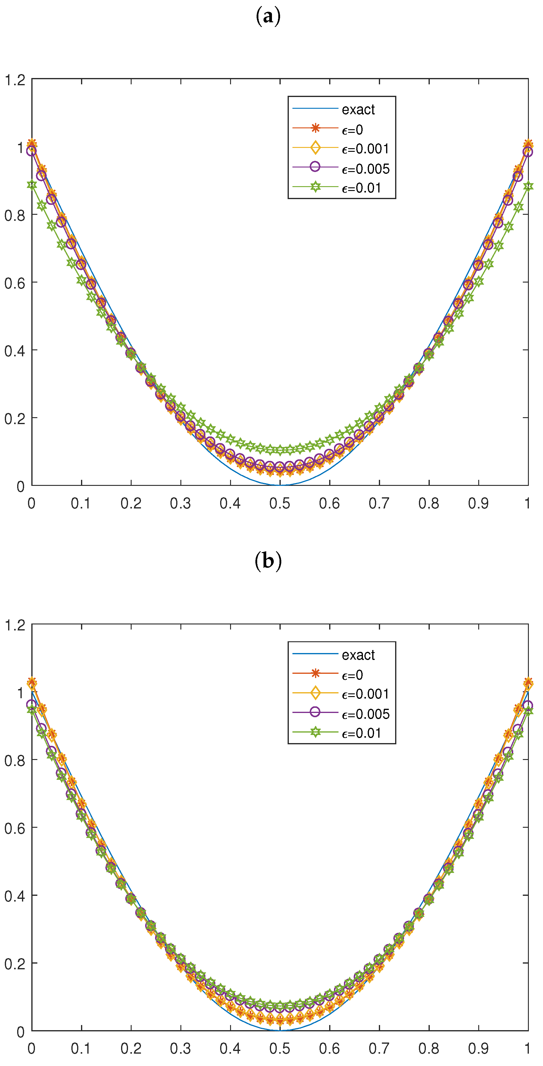
Example 1.

For simulation reasons, we chose $\Omega =(0,1)$, $q_i=1,2,3$, i.e, $p=3.$ For this case, we took the basis function space ${\Phi }_L=span\{1,\sqrt{2}\cos \left(\pi x\right),\cdots ,\sqrt{2}\cos \left((L-1)\pi x\right)\}.$ In the first example, our objective was to identify following example:

$$g\left(x\right)=1-\sin \left(\pi x\right)$$

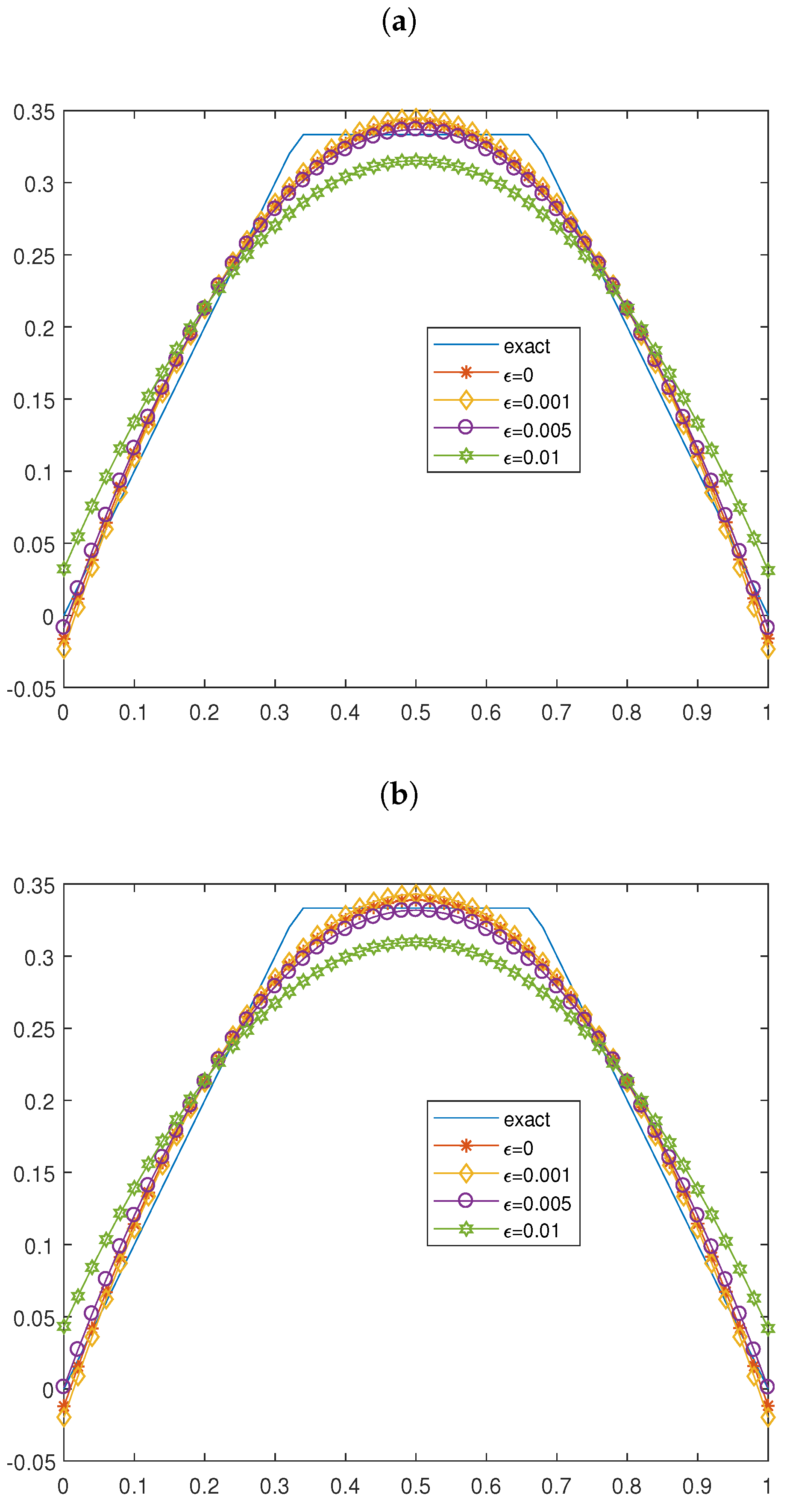
The reconstruction results are shown in Figure 1.

Example 2.

Now, we apply our algorithm to identify the following non-smooth function:

$$g\left(x\right)=\left\{\begin{array}{cc}x,& 0\le x\le {\displaystyle \frac{1}{3}}\\ {\displaystyle \frac{1}{3}},& {\displaystyle \frac{1}{3}}\le x\le {\displaystyle \frac{2}{3}}\\ 1-x,& {\displaystyle \frac{2}{3}}\le x\le 1\end{array}\right..$$

The numerical results of the function, with various noise levels, are illustrated in Figure 2.

From Figure 1 and Figure 2, we see that the space-dependent ST reconstructions for Examples 1 and 2 are very close to the exact terms, i.e., up to 1%. We can also say that our proposed algorithm has a high accuracy for a smooth unknown ST, and the principle of divergence plays an important role for the inversion.

5.2. Two-Dimensional Case

For this case, $x=(x_1,x_2)$, $\Omega =(0,1)\times (0,1)$, $q_i=1,2,3$ and ${\Phi }^{L_1\times L_2}=\left\{{\psi }_i\left(x_1\right){\psi }_j\left(x_2\right)\right\},$ with

$${\psi }_i\left(x_1\right)=\left\{\begin{array}{ccc}1& if& i=1\\ \sqrt{2}\cos \left((i-1)\pi x\right),& i>1\end{array}\right.$$

and

$${\psi }_i\left(x_2\right)=\left\{\begin{array}{ccc}1& if& j=1\\ \sqrt{2}\cos \left((j-1)\pi x\right),& j>1\end{array}\right.$$

$i=1,2,\cdots ,L_1$, $j=1,2,\cdots ,L_2.$

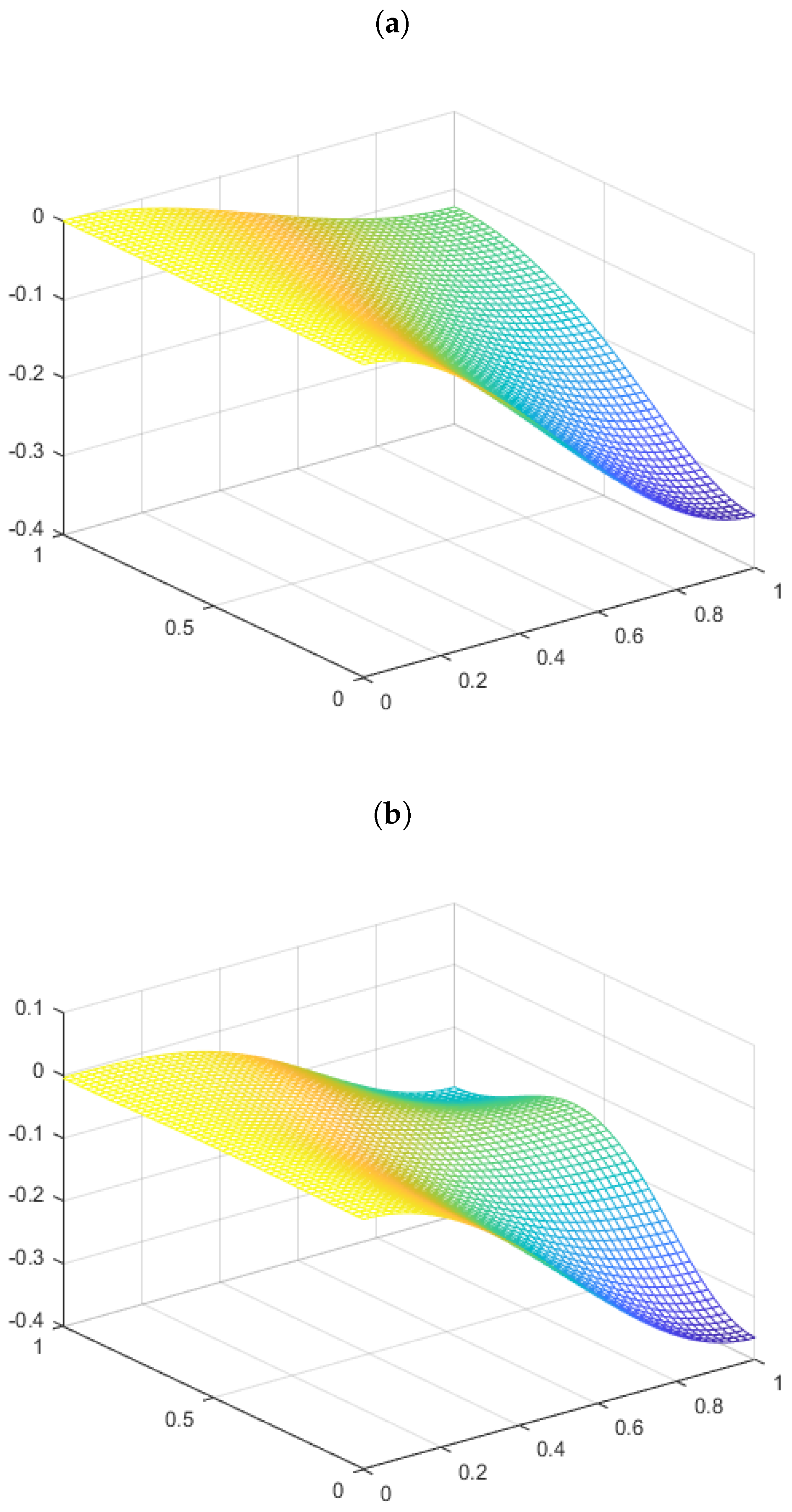
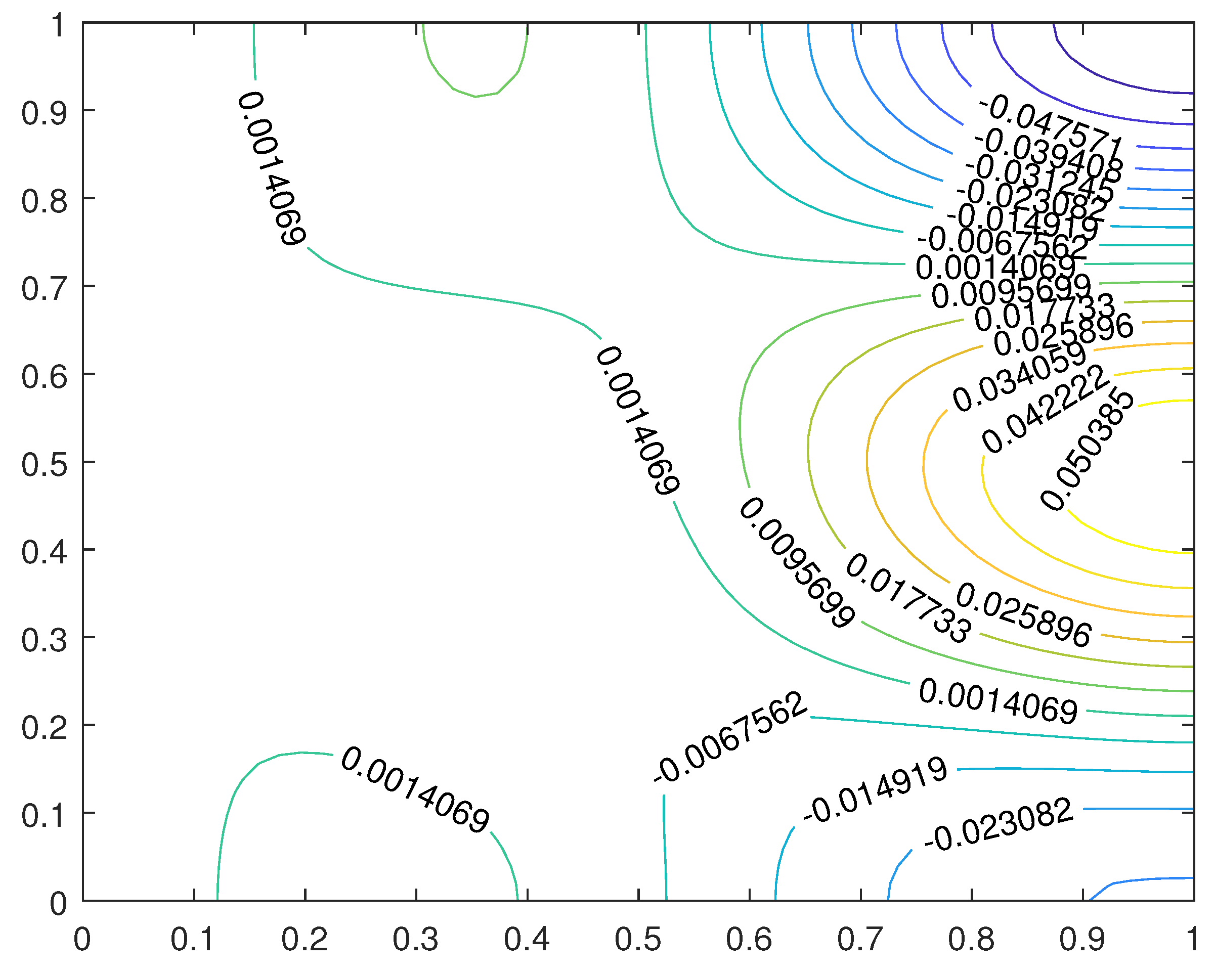
Example 3.

Let us consider the following function:

$$g(x_1,x_2)=\exp \left(\left(2x_2^3-3x_2^2\right)\left({\displaystyle \frac{2}{3}}{x}_1^3-x_1^2\right)\right)$$

(27)

Let $\alpha =(0.9,0.6,0.4)$ and $s=1.2.$ Figure 3 and Figure 4 show the graphs of the exact source, reconstructed STs, and the discrepancies in source terms between the exact values and numerical approximations, when $ϵ=0.01$

Figure 3 and Figure 4 show that the suggested method always has reasonably accurate numerical solutions in the two-dimensional case.

The numerical experiments conducted in one- and two-dimensional cases validated the effectiveness of the proposed method for the reconstruction of inverse source terms. The following observations summarize the main findings and their significance:

• Accuracy of ST reconstruction: The method reconstructs smooth source terms with high accuracy, even in the presence of noise. This confirms its reliability for cases where the underlying source function is continuous and differentiable;
• Non-smooth ST management: Despite the presence of discontinuities, the method accurately captures the main features of non-smooth source terms. This shows its adaptability to irregular real data, where source terms can show abrupt variations;
• Performance in two-dimensional cases: The algorithm maintains a high accuracy and stability when applied to two-dimensional problems. The strong agreement between the reconstructed and exact source terms confirms its ability to be generalized to inverse problems of higher dimensions;
• Error analysis and robustness to noise: The error analysis (e.g., the $L^2$ standard and the convergence of the residual error) confirms the robustness of the approach. The results show that the method is noise resistant, making it a reliable tool for practical applications where data are often noisy;
• Effectiveness of the Levenberg–Marquardt regularization: The Levenberg–Marquardt regularization method plays a key role in stabilizing the opposite problem. It ensures convergence towards an optimal solution while avoiding over-fitting to noisy data. This underscores its effectiveness as a powerful tool for fractional-scattering inverse problems.

These results confirm the applicability of the proposed method in areas such as biomedical imaging, environmental modeling, and thermal conduction analysis, where accurate and stable inverse solutions are essential.

6. Conclusions

This paper explores the inverse source problem associated with the multi-term time-fractional diffusion equation. Additionally, we formulate the ill-posed inverse problem as a minimization challenge and investigate the presence of a minimizer, uniqueness, and stability within this framework. To address the regularized variational problem that incorporates a space-dependent ST, we employed the Levenberg–Marquardt method. During the simulation phase, we evaluated the effectiveness of the proposed approach by numerically reconstructing four distinct examples in one- and two-dimensional scenarios. These simulations served to showcase the precision and efficiency of the proposed methodology.