Appendix B. Proofs of Lemmas
This section lists the main proofs of the lemmas in the paper.
Proof of Lemma 2. For each , solving , we can find a solution of . If , then ; if not, then .
Next, we prove . Note that is a strictly decreasing function of . Hence, for implies or . We then derive for ; we have , and thus . Moreover, for , we have or . Hence, we derive . Combining with , we derive .
Consequently, we have . Meanwhile, and are mutually exclusive. Moreover, the definitions of and imply that and are mutually exclusive. We then derive that , , and are mutually exclusive.
It is concluded that , , and constitute a precision partition for . □
Proof of Lemma 3. Assume ; then, .
Taking the first derivative of
with
yields
where
and
.
Note that for all . Hence, for all , . In other words, strictly decreases with . Combining with , subject to . Since is a continuous function with and , for , and ; we have and , where are arbitrarily small and greater than 0. In addition, and depend on .
In summary, given , we have . Moreover, , ; we derive and . □
Proof of Lemma 4. We divide the proof into two parts.
(1) We prove the given ; then, , .
Recall the expression of the first derivative of
in (
A2). If
, we have
. Recall
. For
,
,
, which implies
. Combining with Lemma 3, we have
.
(2) Taking the first derivative of
with
yields
Note that for all . Combining with , we have for all , which implies for all . Combining with , we have for all , which implies . Hence, and . □
Proof of Lemma 5. Recall
increases with
and
for
. Based on the expression of
in (
A3), we derive that
strictly decreases with
.
Given , we have . Combining with , there must exist a unique subject to . We derive if and if .
Combining with , we derive . Since is a strictly decreasing function of if , there must exist a unique subject to . We then derive if and if . Hence, we derive .
Note that the sets and are mutually exclusive. We have if . Therefore, any precision in the set is lower than any precision in the set . □
Proof of Lemma A1. Definition 2 implies that rational investors need to solve the following optimization problem for information acquisition:
Proposition 5 implies that when all rational investors acquire
, their net expected gain is equal to zero, i.e.,
where allocation
denotes that all rational investors acquire
and the price informativeness is
Due to
, we derive
. Note that the net expected gain
is a concave function with
given allocation
. Combining with
, the net expected gain of a rational investor with precision
given allocation
meets the condition
Next, we prove that all rational investors’ net expected gain is equal to zero in the information market equilibrium.
Suppose that all rational investors acquire a level of precision from
. Meanwhile, the corresponding allocation is denoted as
. We then have
where
.
Furthermore, due to
, we derive
Hence, given allocation
, the net expected gain of a rational investor with precision
satisfies
In other words, the net expected gain of rational investors with precision given any allocation is always less than or equal to zero.
Moreover, rational investors can always choose to be uninformed and have zero net expected gain. Since all rational investors have identical net expected gain in information market equilibrium, we then derive that all rational investors must have zero net expected gain in equilibrium.
Finally, we claim that all informed agents choose the same precision level in information market equilibrium.
It is assumed that equilibrium is characterized by allocation . Rational investors can acquire at most two various levels of precision with the same net expected gain because the net expected gain is a concave function with precision given allocation . Moreover, Definition 2 implies all rational investors have identical net expected gain in information market equilibrium. Combining with , we derive that there exists only one level of precision such that . Hence, all informed agents acquire identical precision levels in equilibrium. □
Appendix C. Proofs of Propositions
This section lists the main proofs of the propositions in the paper.
Proof of Proposition 1. For notation simplification, we use , , and p to substitute for , , and .
Consider the linear strategy. From Equations (
5) and (
6), the demands for informed agents and uninformed agents can be rewritten by
and
.
Combining with the market-clearing condition shown in Equation (
2) yields
, where
,
,
, and
.
Hence, given the linear strategy, the information set is observable equivalent (O.E.) to .
Define
,
. Based on the projection theorem, we have
and
, since
. Going back to Equation (
5), the trading strategy of the informed agent
is given by
where
.
Similarly, since
, going back to Equation (
6), the strategy of the uninformed agent
i is given by
Substituting the expressions of
and
into the market-clearing condition shown in Equation (
2) yields
where
,
.
Combining with (
A14), we rewrite (
A12) and (
A13) by
where
.
Note that we omit some notations as functions of allocation A for notation simplification. These notations are as follows:
,
,
,
,
,
,
, and
. Moreover, the coefficients of
in Equation (
1) are verified by
,
, and
. □
Proof of Proposition 2. We use mathematical induction to complete our proof. The total proof is divided into three parts.
We consider a scenario where the information market features two sellers denoted as and information precision set only contains two elements, and (i.e., Scenario ). Meanwhile, rational investors need to make their optimal information acquisition decisions from the set .
We first judge whether the allocation
is an information market equilibrium. There are four possible types of allocation
illustrated in
Figure A1,
Figure A2, and
Figure A3, respectively.
In
Figure A1, each type of allocation
is a non-zero corner equilibrium because
and all investors have identical net expected gain.
In
Figure A2, the third type of allocation
is not an information market equilibrium because
. We then turn to verify whether the allocation
is an information market equilibrium. There are four possible evolutionary routes for allocation
given this type of allocation
. Each evolutionary route leads to a non-zero corner equilibrium.
In evolutionary route a, allocation is a non-zero corner equilibrium because and all rational investors have identical net expected gain.
In evolutionary route c, although allocation is not an information market equilibrium (see ), we can find a non-zero corner equilibrium characterized by another allocation where a part of the rational investors acquire and others acquire . Moreover, allocation can be built in the following ways:
Expanding
yields
where
,
.
(
A17) implies that
is a strictly increasing function with
.
and
implies there exists a value of
such that
where
,
,
.
Similarly, we can analyze a non-zero corner equilibrium in evolutionary route b and a non-zero corner equilibrium in evolutionary route d.
In
Figure A3, there are three various evolutionary routes given the fourth type of allocation
. Similarly, allocation
in evolutionary route a and allocation
in evolutionary routes b and c are non-zero corner equilibria, respectively.
We conclude there exists a non-zero corner equilibrium in the information market where two sellers produce precision and . In the equilibrium, all rational investors acquire identical precision, or a part of the investors acquire and others acquire .
It is assumed that there exists a non-zero corner equilibrium in the scenario where the information market features
sellers with the precision set
(i.e., Scenario
). Meanwhile, the equilibrium is characterized by an allocation
or an allocation
, where
. The allocation
denotes that all rational investors acquire
. The allocation
denotes that a part of the investors acquire
and others acquire
. Meanwhile,
and
satisfy
We attempt to analyze the existence of information market equilibrium in a situation where the information market features sellers with a precision set (i.e., Scenario ), by using the assumption depicted in Part 2.
Case 1: It is assumed that there is a non-zero corner equilibrium characterized by allocation in the Scenario .
(1) Suppose .
There are a total of two possible types of allocation
illustrated in
Figure A4. We find that each type of allocation
indicates a non-zero corner equilibrium in the Scenario
. This occurs because
.
(2) Suppose .
There are a total of four possible types of allocation
. The fourth type of allocation
is similarly analyzed as the allocation
illustrated in
Figure A2. We focus on the other three types of allocation
illustrated in
Figure A5 and
Figure A6.
In
Figure A5, each type of allocation
is a non-zero corner equilibrium because
.
In
Figure A6, the third type of allocation
has three various evolutionary routes. In evolutionary route a, allocation
is a non-zero corner equilibrium; in evolutionary routes b and c, allocation
is a non-zero corner equilibrium.
Hence, we conclude that if there exists a non-zero corner equilibrium characterized by in the Scenario , we will derive that there exists a non-zero corner equilibrium in the Scenario .
Case 2: It is assumed that there is a non-zero corner equilibrium characterized by the allocation in the Scenario .
Combining and , we derive . Therefore, allocation is still a non-zero corner equilibrium in the Scenario .
We have completed our mathematical induction through the above proof. First, we prove there exists a non-zero corner equilibrium in the Scenario . Second, we assume there exists a non-zero corner equilibrium in the Scenario . Third, given the assumption, we derive that there exists a non-zero corner equilibrium in the Scenario . Hence, when the information market features sellers, there always exists a non-zero corner equilibrium characterized by the allocation shown in Proposition 2. □
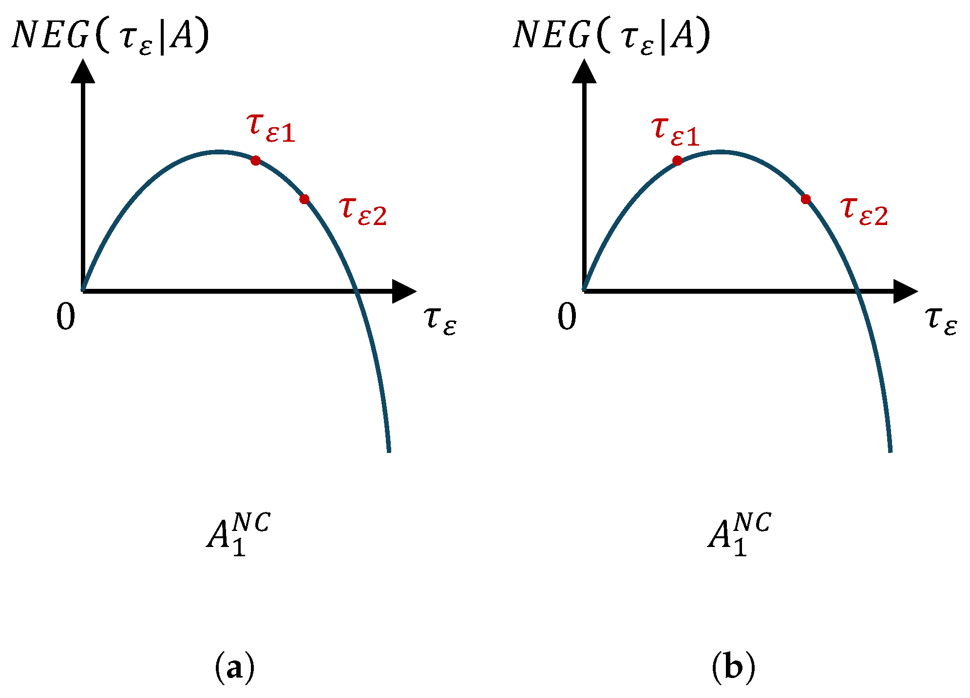
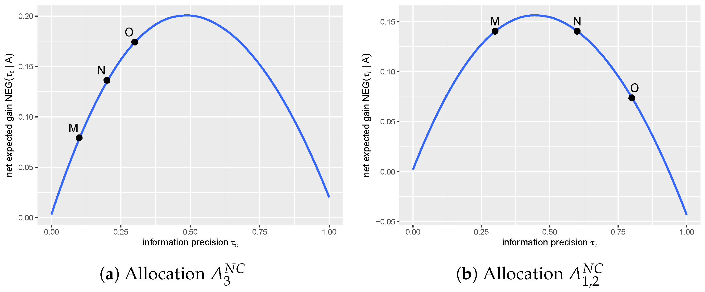
Figure A1.
The relationship between the net expected gain and information precision given two different types of allocation . Panels (a,b) characterize the first and second types of allocation , respectively. In both panels, the position of the point is higher in vertical height than the point given an allocation A, implying .
Figure A2.
The relationship between the net expected gain and information precision given the third type of allocation . In the figure, the orange lines denote potential evolutionary routes. An allocation in bold black in an evolutionary route indicates an information market equilibrium. For instance, allocation in bold black in route a is a non-zero corner equilibrium. Specifically, allocation denotes that a part of the rational investors acquire and others acquire . Moreover, the position of the point is higher in vertical height than the point given an allocation A, implying .
Figure A3.
The relationship between the net expected gain and information precision given the fourth type of allocation . In the figure, the orange lines denote potential evolutionary routes. An allocation in bold black in an evolutionary route indicates an information market equilibrium. For instance, allocation in bold black in route a is a non-zero corner equilibrium. Specifically, allocation denotes that a part of the rational investors acquire and others acquire . Moreover, the position of the point is higher in vertical height than the point given an allocation A, implying .
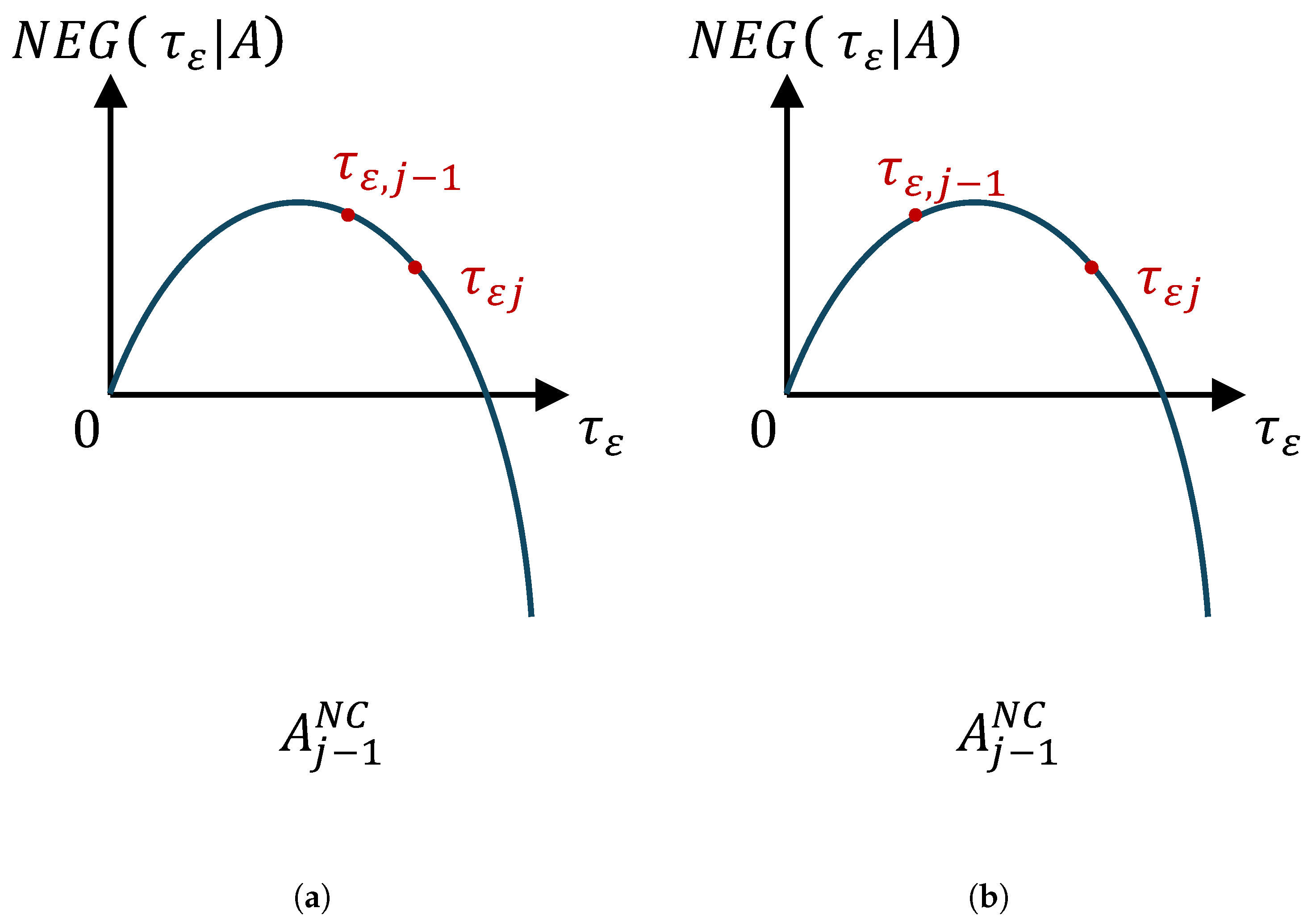
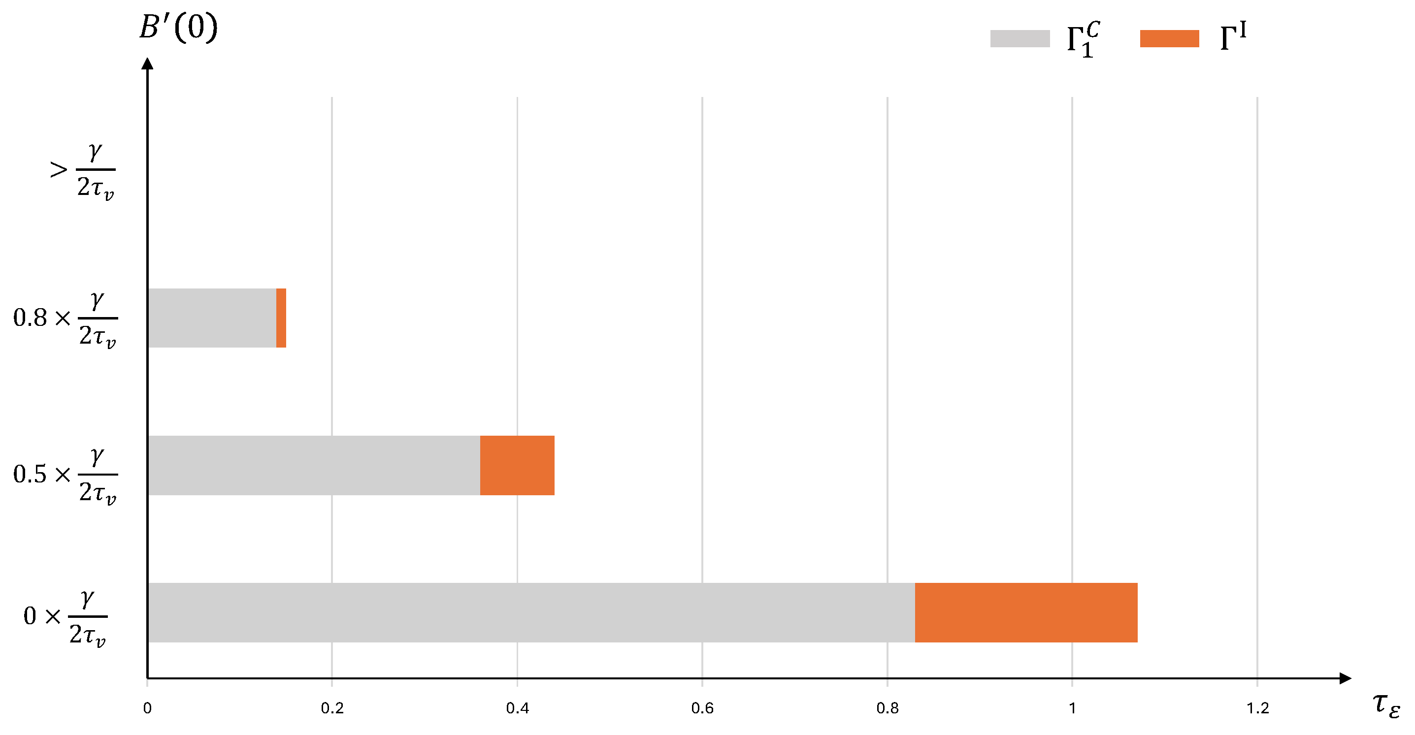
Figure A4.
The relationship between the net expected gain and information precision given two different types of allocation . In the figure, Panels (a,b) represent the first and second types of allocation , respectively. In both panels, the position of the point is higher in vertical height than the point given an allocation A, implying . Points between and are ignored.
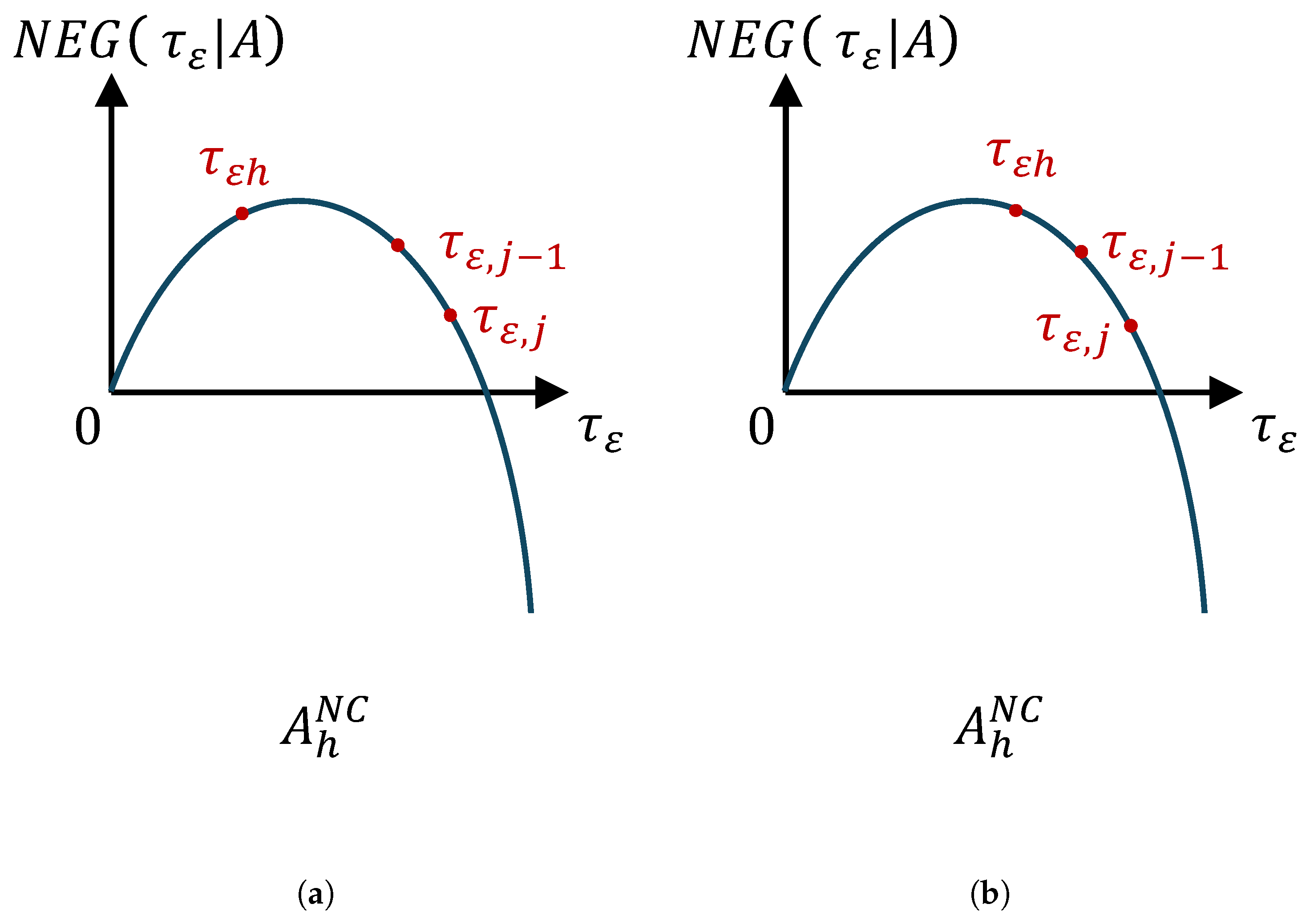
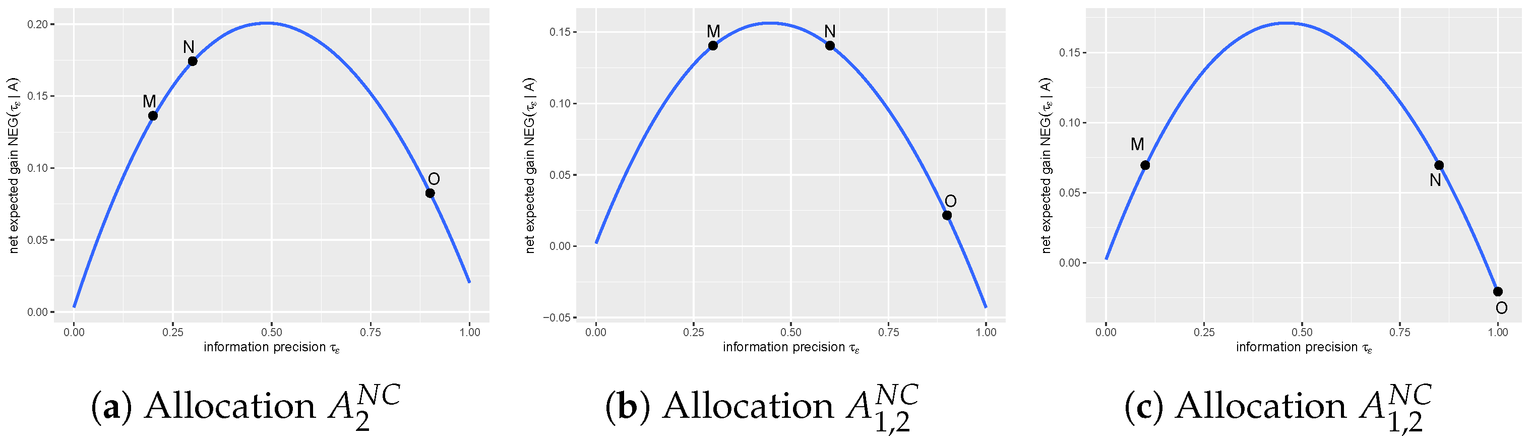
Figure A5.
The relationship between the net expected gain and information precision given two different types of allocation . In the figure, Panels (a,b) represent the first and second types of allocation , respectively. In both panels, the position of the point is higher in vertical height than the point given , implying .
Figure A6.
The relationship between the net expected gain and information precision given the third type of allocation . In the figure, the orange lines denote potential evolutionary routes. An allocation in bold black in an evolutionary route indicates an information market equilibrium. For instance, allocation in bold black in route a is a non-zero corner equilibrium. Specifically, allocation denotes that a part of the rational investors acquire and others acquire . Moreover, the position of the point is higher in vertical height than the point given an allocation A, implying .
Proof of Proposition 3. Based on Lemma A1, there is only one precision level in information market equilibrium. In the following, we examine whether allocation where is an information market equilibrium.
We divide our proof into three sub-proofs. First, we prove is equivalent to ; second, we prove there exists a unique such that ; third, we prove that the price informativeness when all informed agents acquire .
We prove . We divide our proof into two parts.
(1) .
For
, the net expected gain of informed agents with precision
given
satisfies
Due to , we derive . Hence, , .
Moreover,
implies that
. We then derive
(2) .
Note that
. For
, we have
Expanding
yields
Due to
, we can always find an allocation
such that
. Expanding
yields
Comparing the coefficients of (
A23) and (
A24) yields
.
The above two parts of the proof imply that is equivalent to .
We prove that there exists unique precision such that .
Since has finite elements, we can always find such that .
It is assumed that there is another precision
such that
. The net expected gain of informed agents with precision
given allocation
satisfies
Note that the net expected gain of informed agents with precision
given
satisfies
We then have .
Note that the net expected gain of uninformed agents is always equal to zero (see ). As a result, implies because is a concave function with precision given . This is in contrast with our assumption that . Thus, the optimal precision , which maximizes price informativeness, is unique.
We prove when all informed agents acquire .
Combining with , as a concave function, we derive that decreases with , where .
Due to
, where
, we derive
Since
,
. We have
Comparing the coefficients of the left-hand and right-hand sides yields
which implies
. □
Proof of Proposition 4. We first show that allocation
,
is not an information market equilibrium. Note that
.
as a concave function implies that
for
. We then have
Hence, allocation is not an information market equilibrium.
Next, we indicate that each type of allocation leads to an information market equilibrium, where allocation denotes the “equilibrium allocation” in the scenario in which rational investors can only choose precision from the set . As , by using the result in Proposition 2, we derive that allocation is equal to allocation , where , or allocation , where .
Suppose that
, where allocation
satisfies
(1) Consider .
Note that
is a concave function with given allocation
. Due to
and
,
, we derive
Combining with (
A32), we derive allocation
as a non-zero corner equilibrium.
(2) Consider .
(a) Suppose .
Therefore, allocation is a non-zero corner equilibrium.
(b) Suppose .
Since
, we have
. Combining the fact that
is a concave function with given
and
yields
Note that
for
. Given
, we derive
Due to
, we have
Comparing the coefficients of (
A37) and (
A38) yields
. Due to
, we then have
Moreover, given an allocation
A, expanding
yields
Since , is a strictly increasing function of .
Combining (
A36) and (
A39) yields
Therefore,
holds. Combining this with the assumption
, we derive that there exists an allocation
where a part of the rational investors acquire
and others acquire
such that
Clearly, allocation
is a non-zero corner equilibrium. This occurs because
Suppose that
, where
Due to the concave feature of
, for
,
, we derive
Hence, allocation is still a non-zero corner equilibrium.
In conclusion, by using the “equilibrium allocation” in the situation where rational investors can only choose precision in the set , there always exists a non-zero corner equilibrium characterized by an allocation satisfying the conditions in Proposition 4. □
Proof of Proposition 5. Given an information precision set , there is a unique interior equilibrium characterized by equilibrium allocation where all informed agents choose the same precision level based on Proposition 3. In this case, price informativeness is denoted as .
As information quality enhances, the precision set changes to ; similarly, there is a unique interior equilibrium characterized by equilibrium allocation where all informed agents choose the same precision level . In addition, price informativeness is denoted as .
Note that ; we then have by using Proposition 3.
As costs of information acquisition decrease, more informed agents will acquire information due to higher information value. Following the expression of price informativeness in Proposition 3, it is concluded that price informativeness increases in financial markets. □
Proof of Proposition 6. Proposition 6 is directly derived from Proposition 3. QED. □

