Abstract
Redundant manipulators (RMs) are widely used in various fields due to their flexibility and versatility, but challenges remain in adjusting their inverse kinematics (IK) solutions. Adjustable IK solutions are crucial as they not only avoid joint limits but also enable the manipulability of the manipulator to be regulated. To address this issue, this paper proposes an IK optimization method. First, a performance metric for adjustable IK solutions is developed by introducing the motion-level factor. By setting the desired joint motion level, the IK solutions can be adjusted accordingly. Furthermore, a two-stage optimization algorithm is proposed to obtain the adjustable IK solutions. In the first stage, a modified gradient projection method is used to optimize the performance metric, generating a set of initial optimal solutions. However, cumulative errors may arise during this stage. To counteract this, the forward and backward reaching inverse kinematics algorithm is employed in the second stage to enhance the accuracy of the initial solutions. Finally, the effectiveness of the proposed method is validated through simulations and experiments using a planar cable-driven redundant manipulator. The results demonstrate that the IK solutions can be adjusted by modifying the motion-level factors. The proposed two-stage optimization algorithm integrates the advantages of the gradient projection method and the forward and backward reaching inverse kinematics algorithm, yielding a set of accurate and optimal IK solutions. Furthermore, the adjustable IK solutions facilitate the regulation of the RM’s manipulability, enhancing its adaptability and flexibility.
MSC:
70B15; 53A17; 65K10
1. Introduction
Redundant manipulators (RMs) have gained significant attention due to their greater number of degrees of freedom (DOFs) than the minimum required to perform a task [1]. Unlike traditional manipulators that possess only the minimum DOFs required to complete a task, RMs offer an expanded workspace along with enhanced flexibility and adaptability [2,3,4]. This surplus of DOFs allows RMs to accommodate additional functional constraints while simultaneously performing their primary tasks [5]. With these advantages, RMs are well-suited for a wide range of complex scenarios, including spacecraft maintenance [6], nuclear reactor maintenance [7], aeroengine inspection [8,9], and medical surgery [10,11].
Despite their numerous advantages, RMs present significant challenges due to the excess DOFs, which render the IK problem ill-posed [12]. The nature of redundant DOFs typically leads to multiple feasible inverse kinematic solutions for a given End-effector pose. Therefore, IK optimization for a specific pose is a crucial issue in the study of RMs. To address this challenge, researchers have proposed optimizing various performance metrics, including avoiding joint limits [13,14], minimizing joint torque [15,16], and maximizing manipulability [17,18]. Among these metrics, respecting joint limits is a fundamental principle in IK solutions. Since joint variables are constrained by mechanical limits, violating these limits can result in mechanical boundary collisions or structural damage. When joints reach their limits, semi-singularity issues arise, which are more complex to handle than kinematic singularities [19]. Therefore, avoiding joint limits remains a classic and critical issue in the IK optimization of RMs.
In previous studies, a performance metric for avoiding joint limits was proposed in [20]. However, this metric does not directly indicate whether a joint has reached its limits. To address this limitation, a new performance metric for joint limit avoidance was introduced in [21]. This metric approaches infinity as the joint limits are reached, achieves its minimum value at the midpoint of the joint range, and has been widely adopted in various methods for avoiding joint limits [14,22,23,24]. Most of the existing studies solve the IK problem using Jacobian-matrix-based optimization methods, where the problem is addressed in the velocity domain. A typical method is the gradient projection method (GPM), which has been extensively applied in joint limit avoidance [20,21,25,26,27]. These velocity-based optimization methods for the IK problem require integrating angular velocities over time. The prolonged integration process can result in accumulated errors, leading to deviations in the final results in the position domain. On the other hand, some studies have proposed methods for directly solving the IK problem in the position domain. These methods avoid the accumulated errors in the velocity integration process, offering a more accurate assessment of the manipulator’s state in the task space. Some studies derived closed-form IK solutions for specific redundant manipulators in the position domain [28,29,30]. Additionally, the forward and backward reaching inverse kinematics (FABRIK) algorithm proposed in [31], which solves the IK problem through geometric iterations, can rapidly reach the target pose and is unaffected by singularity issues. The FABRIK algorithm has been widely applied to cable-driven segmented manipulators [32], multi-segment continuum robots [33], and continuum robots [34]. However, these methods have certain limitations. Specifically, methods [25,26,27] require time integration to obtain joint angles, which can introduce accumulated errors, leading to inaccurate solutions. Methods [28,29,30] are limited to specific manipulator structures and cannot accommodate arbitrary configurations. Methods [31,32,33,34] rely on geometric iteration without global search capability, preventing them from ensuring the identification of the optimal solution. In contrast, this paper introduces a novel IK optimization method for RMs that prioritizes both accuracy and optimality. The goal is to obtain a set of accurate and optimal IK solutions.
Although the aforementioned studies have made significant progress in IK optimization, no research has yet addressed the adjustable IK problem for RMs while avoiding joint limits and singularities. In various application scenarios, IK solutions often need to be adjusted to satisfy different requirements. Therefore, research on adjustable IK solutions for RMs is essential. This paper proposes a novel IK optimization method for RMs, aiming to achieve adjustable IK solutions that avoid both joint limits and singularity issues. A performance metric for adjustable IK solutions is developed by introducing the motion-level factor, which allows the IK solutions to be adjusted by modifying this factor. We propose a two-stage optimization algorithm to compute adjustable IK solutions by integrating velocity-based and position-based IK approaches. In the first stage, a modified GPM is employed to optimize the performance metric for adjustable IK solutions, generating a set of initial optimal solutions. In the second stage, the FABRIK algorithm is applied to refine the initial solutions, effectively eliminating the cumulative errors generated in the first stage. The proposed method combines the advantages of both velocity-based and position-based IK methods, not only enabling the generation of adjustable IK solutions but also significantly improving their accuracy.
The contributions of this work are summarized as follows:
- To achieve adjustable IK solutions, we develop a performance metric by introducing a motion-level factor. By customizing this factor, the IK solutions can be tailored to meet specific requirements.
- To obtain adjustable IK solutions, we propose a two-stage optimization algorithm. This algorithm not only generates adjustable IK solutions but also significantly enhances their accuracy.
- The manipulability of an RM is a function of the joint variables. By adjusting the motion-level factor, manipulability can be regulated.
The paper is organized as follows: Section 2 presents the problem formulation. Section 3 presents a two-stage optimization algorithm for adjustable IK solutions. Section 4 illustrates the proposed method using a planar cable-driven redundant manipulator. Section 5 presents numerical simulations of the proposed method. Section 6 offers experimental validation, and Section 7 concludes this paper.
2. Problem Formulation
2.1. Kinematics Model
For an RM with n DOFs, the relationship between the joint space and the task space can be expressed as:
where represents the End-effector pose vector in the task space, represents the joint variables, and represents the nonlinear function used for forward kinematics calculations.
Taking the time derivative of both sides of (1), the linear relationship between the End-effector velocity and joint velocity can be expressed as follows:
where represents the Jacobian matrix, which can be calculated as follows:
2.2. Problem Formulation
For an RM, (2) is underdetermined. As a result, a given End-effector pose may correspond to infinitely many feasible IK solutions. IK resolution of RMs is typically formulated as a constrained optimization problem. The kinematics of RMs in the position domain involve a nonlinear mapping, which increases the difficulty of solving the IK problem. In contrast, kinematics in the velocity domain provide a linear mapping, making them commonly used as equality constraints in the optimization problem. To ensure the solution satisfies the physical limits of the joints, these limits are incorporated as inequality constraints. Therefore, considering both the joint limits and (2), the IK optimization problem can be formulated as follows:
where and represent the lower and upper limits of the joint variables , respectively. and represent the lower and upper limits of the joint velocity , respectively.
3. Two-Stage Inverse Kinematics Optimization
In this section, we develop a performance metric for adjustable IK solutions by introducing the motion-level factor. To obtain the adjustable IK solutions for each End-effector pose, a two-stage optimization algorithm (TSOA) is proposed. In the first stage, a modified GPM is employed to obtain a set of initial optimal solutions. In the second stage, the FABRIK method is applied to enhance the accuracy of the initial solutions. This algorithm enables the generation of adjustable IK solutions while avoiding joint limits and singularity issues.
3.1. Performance Metric
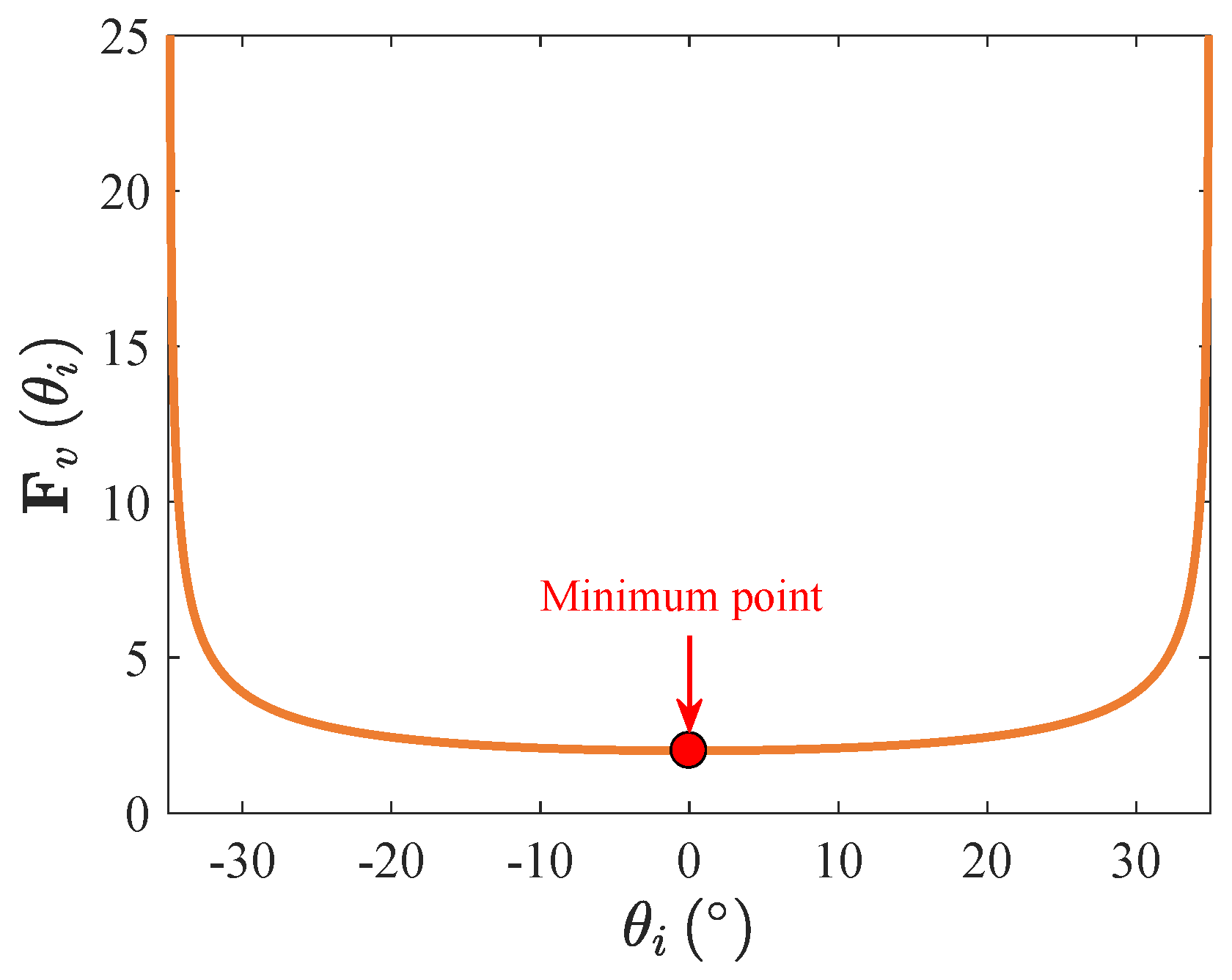
The performance metric for joint limit avoidance can be expressed as follows:
where , , , and represent the elements of , , and , respectively.
Figure 1 illustrates the distribution of the performance metric within the joint limits. It can be observed that the minimum value of occurs at the midpoint of the joint limits (as indicated by the red marker). As the approaches the upper or lower limits, tends to infinity. Therefore, by minimizing the performance metric , the IK solutions that avoid joint limits can be obtained.
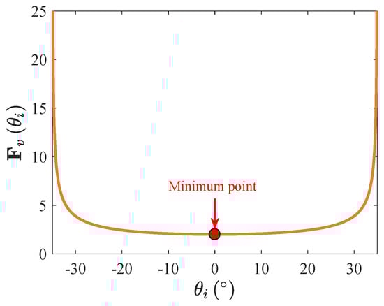
Figure 1.
Value of for joint.
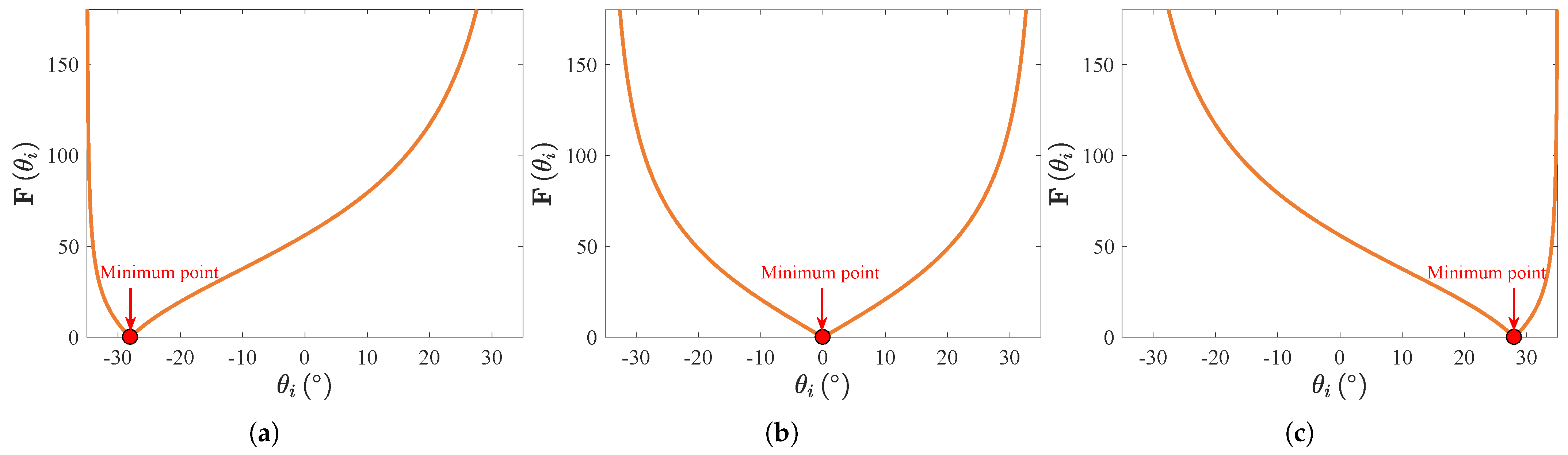
It is desirable to adjust the IK solutions of RMs to meet varying task requirements. However, the performance metric alone cannot achieve IK solutions adjustment. To address this limitation, this paper introduces the motion-level factor into performance metric , enabling the generation of adjustable IK solutions. The performance metric for the adjustable IK solutions can be expressed as follows:
where represents the joint motion adjustment term, which is defined as follows:
where represents the motion-level factor of the joint. By adjusting the value of , the motion level of the joint within its limits can be defined.
Figure 2 illustrates the distribution of the performance metric within the limits of the joint. It can be observed that when , the minimum point of is located at the midpoint of the joint limits, away from both the lower and upper limits. When , the minimum point of is close to the lower limit, while when , the minimum point is close to the upper limit. As the reaches either the upper or lower limit, tends to infinity. These figures demonstrate that can adjust the minimum point of . It is important to emphasize that the motion-level factor serves only as a tool to specify the desired motion level for each joint. However, the IK solutions derived from (4) may not achieve these levels, as they must also satisfy the constraint .
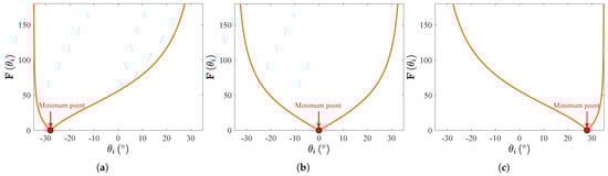
Figure 2.
Value of for joint. (a) . (b) . (c) .
3.2. Stage 1: IK Optimization Based on Modified GPM
3.2.1. Gradient Projection Method
The GPM optimizes the performance metric using the null space of the Jacobian matrix, without affecting the End-effector motion of the manipulator. Specifically, this method projects the steepest descent direction of the performance metric onto the null space of the Jacobian matrix and selects the optimal solution along this projection vector. The minimum value of the performance metric corresponds to the desired optimal solution.
Since , the Jacobian matrix is a non-square matrix. For any given End-effector velocity , the joint velocities can be calculated as follows:
where is the least-norm solution, is the homogeneous solution, which belongs to the null space of the Jacobian matrix . represents the pseudoinverse of . If is full row rank, . is the null space projection matrix, and is an arbitrary joint velocity vector.
By applying the GPM to optimize , with replacing , (9) can be rewritten as follows:
where k is a real scalar, and represents the gradient of , which can be calculated as follows:
If is maximized, the scalar k is positive; conversely, if is minimized, k is negative. A larger value of k results in a faster optimization process.
3.2.2. IK Optimization Model
Since the GPM can only find the optimal solution in the null space, optimizing IK with this method requires transforming the search space into the null space. This transformation can be mathematically represented as
where represents a point in the null space of the Jacobian matrix .
3.2.3. Optimization Algorithm
To avoid joint limits and obtain adjustable inverse kinematic solutions, the problem in (13) is solved using the GPM to find the optimal solution. The specific steps are detailed in Algorithm 1.
The process of searching for the optimal solution within the null space under the transformed joint velocity limits is as follows:
where is the local minimum solution along the direction of the unit projection vector , is the initial point of , and D is the distance between and . The projection vector represents the steepest descent direction and can be calculated as follows:
When , it indicates that no further improvement can be made to the performance metric within the null space, thus yielding the global optimal solution.
| Algorithm 1 Adjustable IK Solutions Optimization Based on Modified GPM |
|
The gradient of can be calculated as follows:
where
3.3. Stage 2: Refinement of Optimal IK Solutions Based on FABRIK
The FABRIK algorithm is a geometry-based heuristic iterative approach that determines joint positions through geometric relationships. It has been proven to exhibit good convergence, high computational efficiency, and the ability to avoid singularity issues in a variety of scenarios. By iterating in the position domain, FABRIK effectively mitigates accumulated errors and achieves high solution accuracy. In this study, the FABRIK algorithm is utilized to enhance the precision of the optimal IK solutions derived in Stage 1. The specific calculation steps are detailed in Algorithm 2. The specific calculations for considering joint limits during the iteration process can be referred to the work in [31].
| Algorithm 2 Refinement of Optimal IK Solutions Based on FABRIK |
|
3.3.1. Forward Reaching
Set the End-effector position to the desired position , and the new joint positions are
where represents the position of the joint.
The distance between the new joint positions can be calculated as follows:
Through forward iteration, the new joint positions can be calculated as follows:
where .
3.3.2. Backward Reaching
Set the initial position point as the reference point , and the new joint positions are
The distance between the new joint positions can be calculated as follows:
Through backward iteration, the new joint positions can be calculated as follows:
where .
4. Case Study Example
To concisely illustrate the proposed method, this section uses a planar cable-driven redundant manipulator (CDRM) as a case study. Notably, the method is equally applicable to RMs in three-dimensional space.
4.1. Structure of the CDRM
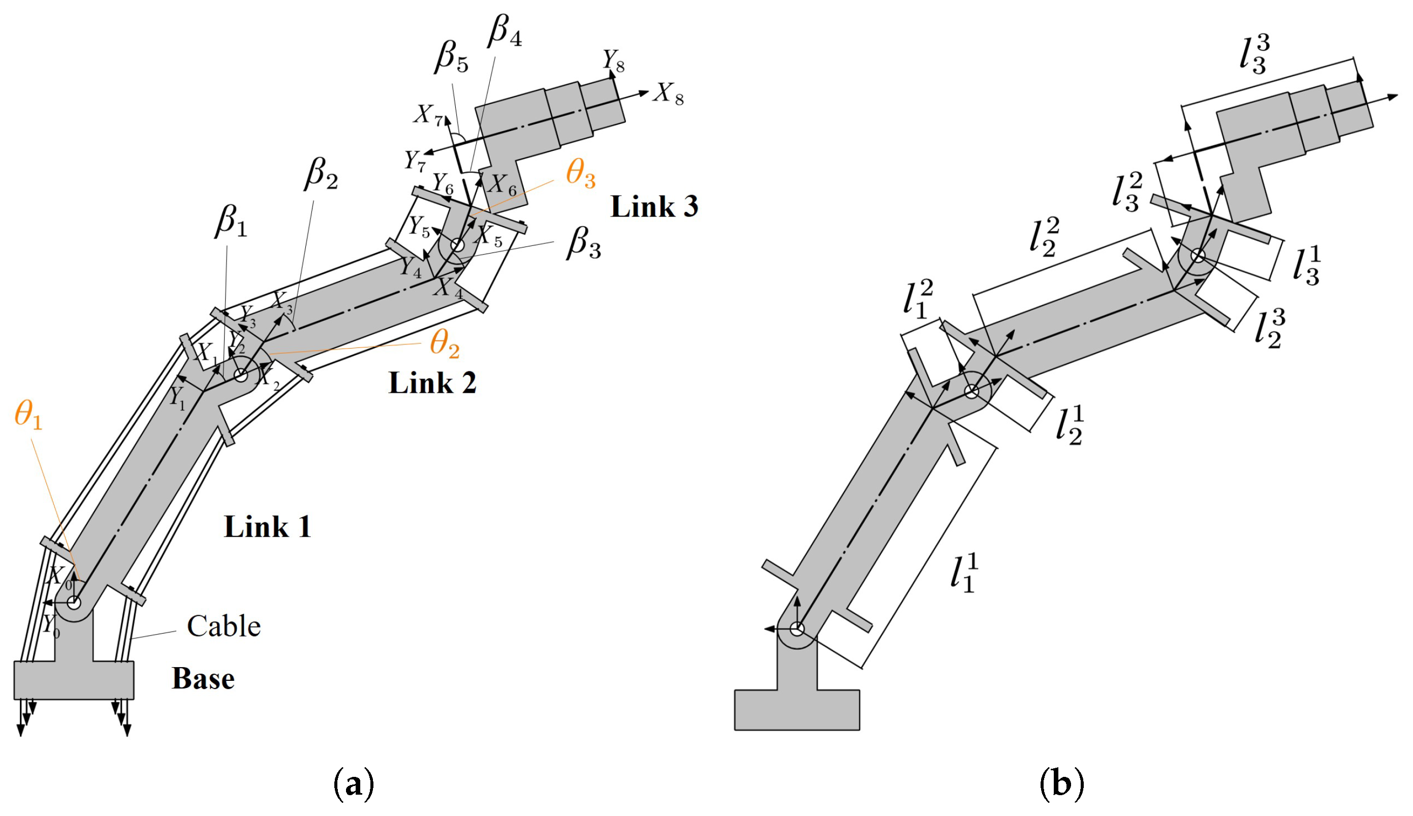
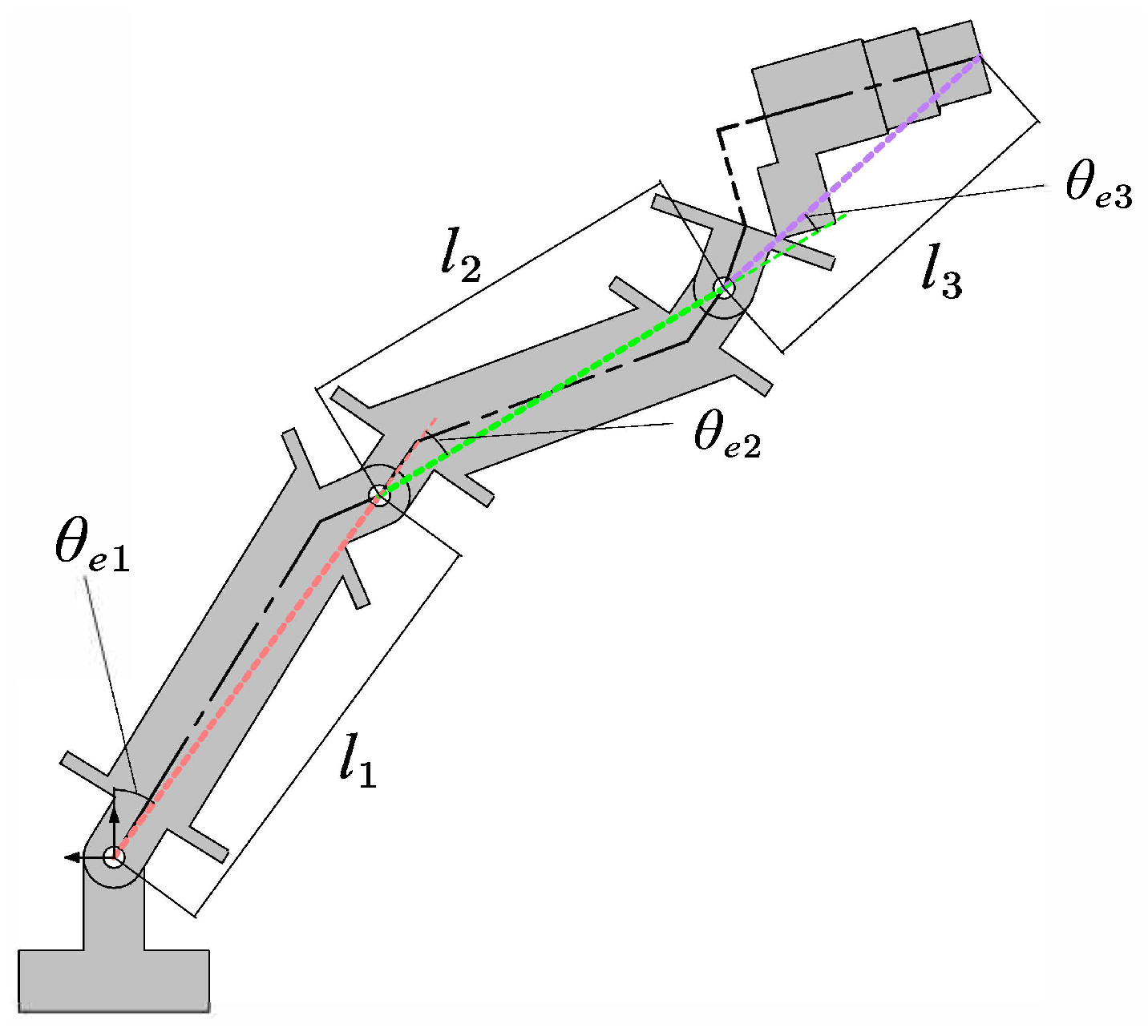
The planar CDRM has three DOFs, but only the position of the End-effector is controlled. Since planar positioning requires only two DOFs, the manipulator possesses one redundant DOF. As shown in Figure 3, the manipulator consists of three rotary joints and three links, and it is driven by six cables. The Denavit–Hartenberg (D-H) frames are established for kinematics analysis of the manipulator, where frame 0 represents the inertial frame, and frame i represents the local frame of each link i. The main parameters of the manipulator are listed in Table 1.

Figure 3.
Planar cable-driven redundant manipulator. (a) D-H frames. (b) Geometric parameters.

Table 1.
Main parameters of the CDRM.
4.2. Kinematic Model
We use the D-H method to establish the kinematic model of the manipulator. The D-H parameters are listed in Table 2. The homogeneous transformation matrix from frame i to frame is expressed as follows:
where .
Table 2.
D-H Parameters of the CDRM.
According to (23), the homogeneous transformation matrix from the End-effector frame to the inertial frame can be calculated as follows:
The End-effector position vector in inertial frame is calculated as follows:
where
Taking the time derivative of both sides of (25), the relationship between the End-effector velocity and the joint velocities can be expressed as follows:
where
4.3. Manipulability
The quantitative measure of the manipulability of a manipulator is defined as follows [35]:
where denotes the singular values of the Jacobian matrix , which can be calculated as follows:
where represents the eigenvalues of , and because is a symmetric positive semi-definite matrix.
When the rank of the Jacobian matrix is less than m, i.e., , the value of w reaches its minimum value of 0, i.e., , indicating that the manipulator is in a singular position where certain movements are impossible to achieve. To avoid singularities and enhance manipulability, it is preferable to select a larger value for w.
However, w reflects only the magnitude of manipulability and does not provide directional information. The condition number of the Jacobian matrix represents the directional information of manipulability and is defined as follows:
where and represent the maximum and minimum singular values of , respectively. A smaller value of indicates better isotropy of the manipulability, signifying that its manipulability is more balanced across different directions.
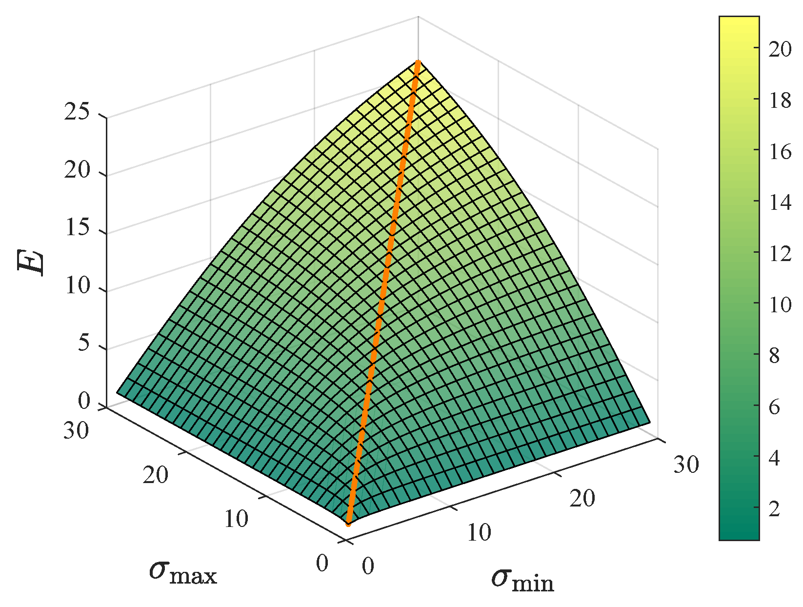
To comprehensively evaluate both the magnitude and directionality of manipulability, a new performance metric is proposed as follows:
The relationship between the performance metric E and the singular values and is shown in Figure 4. When , a ridge line is formed (indicated by the orange line). As and increase, the height of the ridge line also rises. Consequently, a larger E value indicates better manipulability of the manipulator in terms of both magnitude and isotropy.

Figure 4.
Manipulability performance metric.
4.4. Adjustable IK Optimization
4.4.1. Stage 1: IK Optimization
The initial optimal IK solutions are obtained by applying the modified GPM to solve the following optimization problem:
4.4.2. Stage 2: Refinement of Optimal IK Solutions
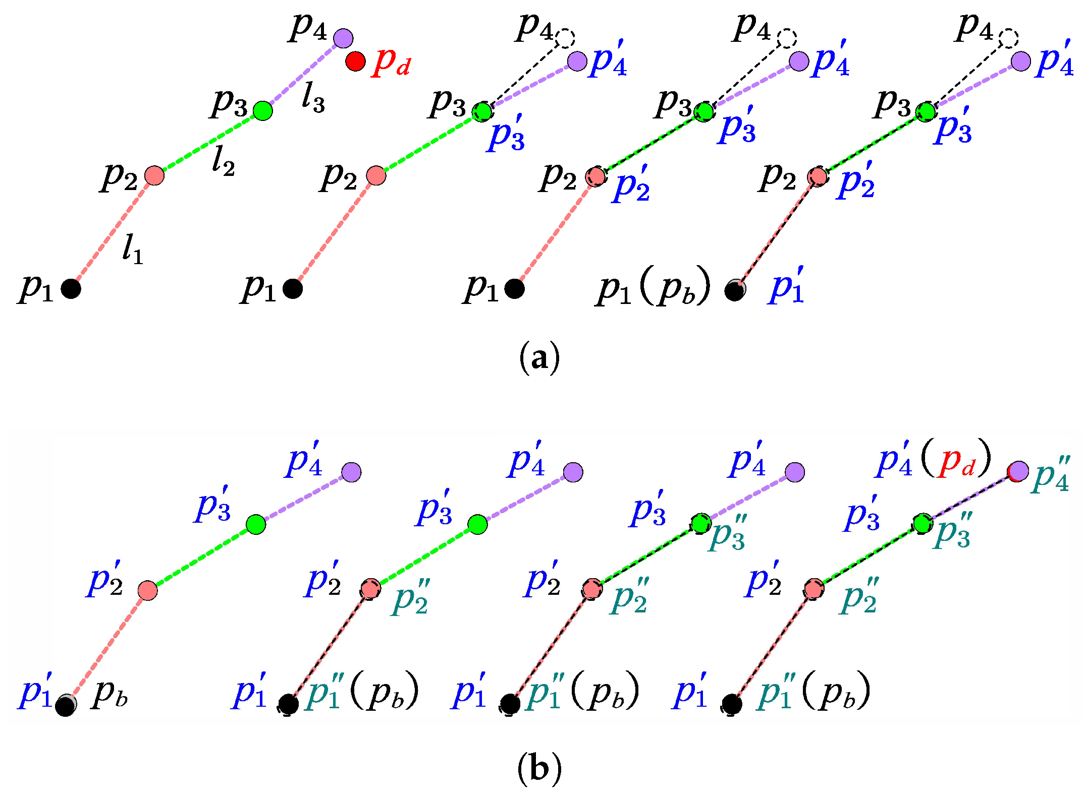
To apply the FABRIK algorithm to the CDRM, the structure of the manipulator is virtually equivalized. The equivalent structure of the manipulator is illustrated in Figure 5, where the equivalent link of link 1 is represented by the orange dashed line, link 2 by the green dashed line, and link 3 by the purple dashed line.
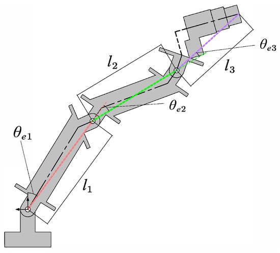
Figure 5.
Equivalence of the CDRM.
Figure 6 illustrates the iterative process of the FABRIK algorithm used to refine the initial optimal IK solutions. This process incrementally adjusts the joint positions of the manipulator, enabling the End-effector to gradually approach the target point, thereby enhancing the accuracy of the initial optimal solutions.
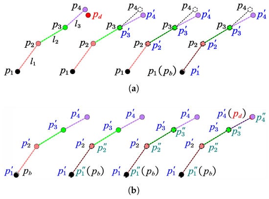
Figure 6.
Iterative process of the FABRIK for refining the initial optimal IK solutions. (a) Forward reaching iteration. (b) Backward reaching iteration.
5. Numerical Simulation
In this section, the effectiveness of the proposed method is demonstrated through numerical simulations. The manipulator’s geometric parameters used in the simulations are listed in Table 1. The motion range of each joint is limited to , and the velocity of each joint is limited to . All algorithms are implemented using Python 3.8.
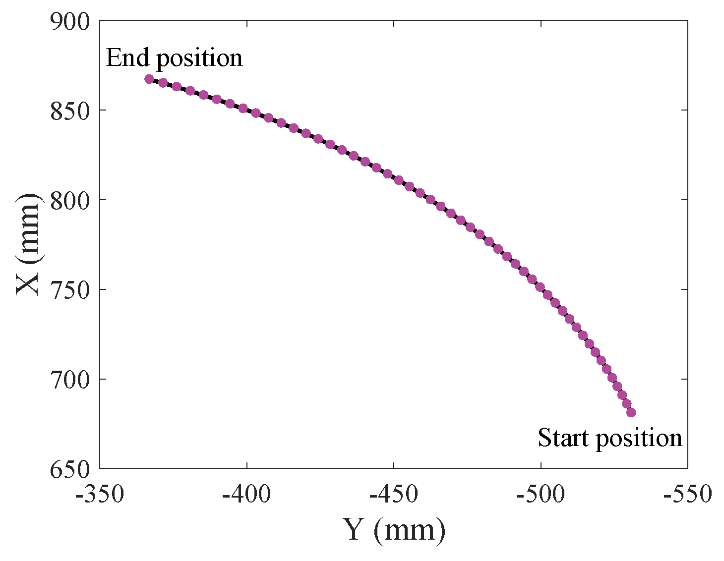
Figure 7 illustrates the motion path of the End-effector in the simulation. To ensure the path remains within the reachable workspace of the manipulator, the first two joint angles are fixed at 5° and 10°, respectively, while the third joint angle is varied from −25° to 25° in 1° increments per step.
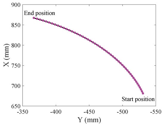
Figure 7.
Motion path.
5.1. Parametric Study
The convergence speed of the GPM is closely related to the choice of the initial point . The initial point must lie within the null space of the Jacobian matrix, as the GPM operates exclusively within it. If the initial point is close to the optimal solution, convergence can occur more quickly. To determine the initial point, the linear programming method (LPM) can be used. Furthermore, the maximum number of iterations is a critical parameter in the GPM. Table 3 shows the convergence results and computation time for various maximum iteration numbers, with the values representing the averages of 20 independent runs. The results indicate that as the maximum iteration number increases, the convergence accuracy improves, but the computation time also increases accordingly. In contrast, fewer iterations reduce computation time but lower the accuracy. After considering both accuracy and computational efficiency, this paper sets the maximum iteration number max_iter to 10.
Table 3.
Average results of convergence errors and computation time for various maximum iteration numbers.
Additionally, the convergence threshold plays an essential role in the FABRIK algorithm, influencing both the stopping criterion and the overall computation time. Table 4 presents the results of the number of iterations and computation time for different convergence thresholds, with the values representing the averages of 20 independent runs. The results show that a larger threshold reduces computation time but may compromise solution accuracy. Conversely, a smaller threshold leads to more iterations and increased computation time. In order to balance both accuracy and computational efficiency, we set the convergence threshold to mm.
Table 4.
Average results of iterations and computation time for different convergence thresholds.
5.2. Accuracy Comparison
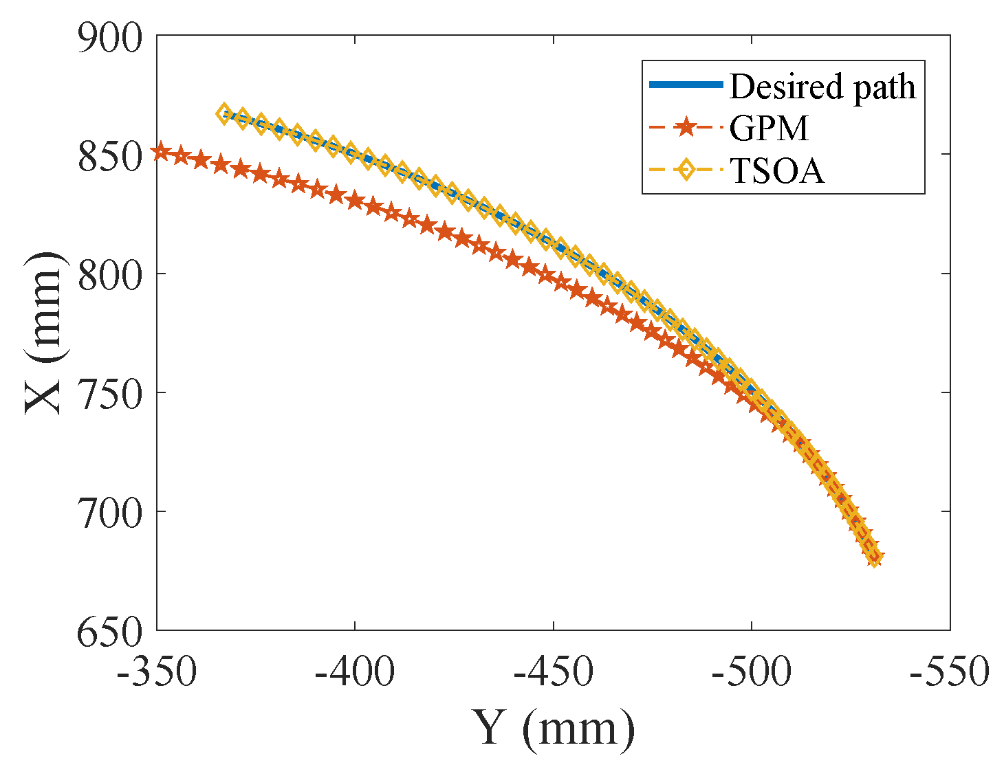
To validate the accuracy of the proposed TSOA, we compared the IK solutions generated by the GPM with those obtained using the TSOA. Figure 8 shows the End-effector trajectories generated by the GPM and TSOA methods compared to the desired path. The trajectory generated by the GPM shows increasing deviations from the desired path as the number of iterations increases, due to the cumulative errors inherent in the method. In contrast, the trajectory produced by the TSOA closely matches the desired path, demonstrating superior accuracy.

Figure 8.
End-effector motion trajectories of different methods.
5.3. Adjustable IK Solutions
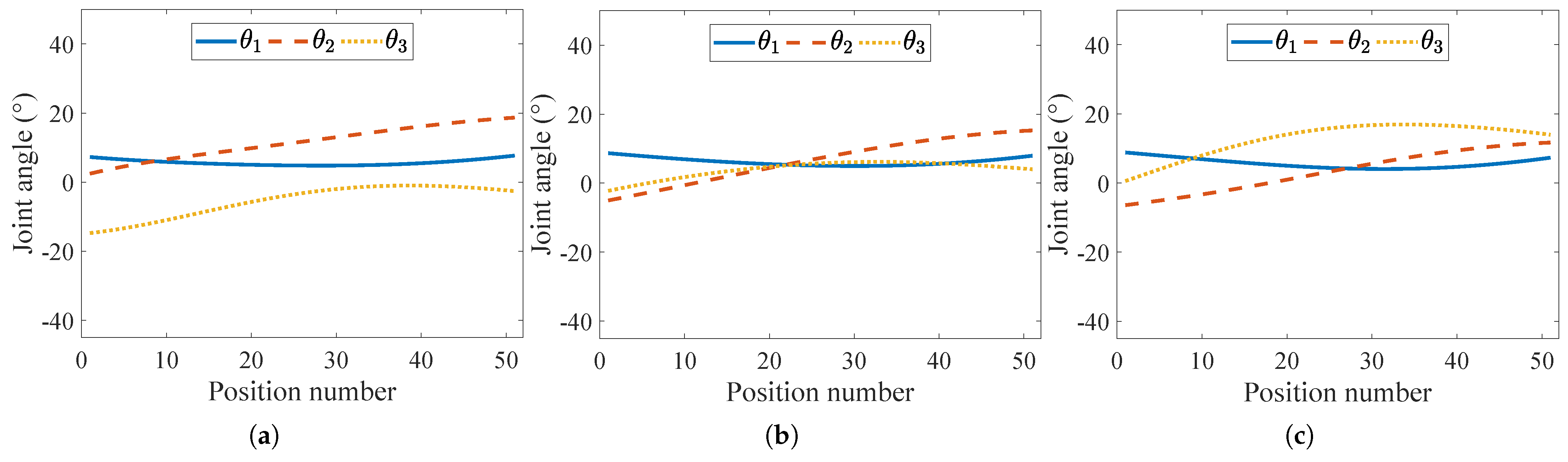
To verify the effectiveness of the proposed method in IK solutions adjustment, Figure 9 shows the IK solutions of the manipulator along the path when the motion-level factor is set to , , and , respectively. It can be observed that when , the solutions are away from both the upper and lower limits of the joint. When , the solutions are close to the lower limit of the joint, while when , the solutions are close to the upper limit.
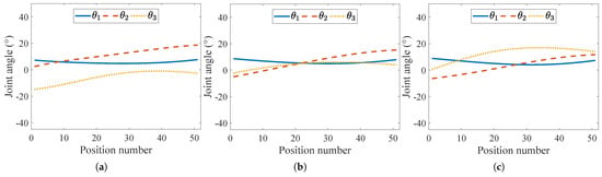
Figure 9.
IK solutions along the path for three different motion-level factors. (a) . (b) . (c) .
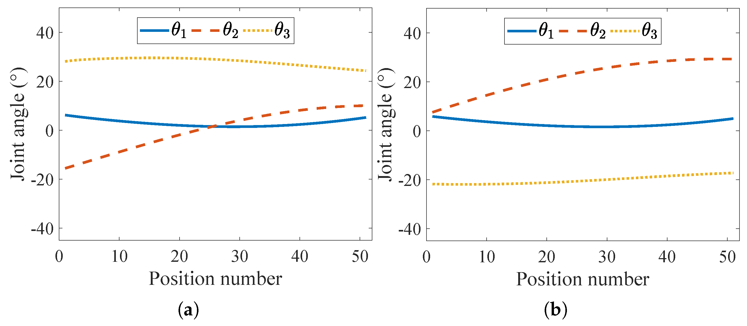
In some cases, it is beneficial to assign different motion levels to each joint. Figure 10 illustrates the IK solutions along the path when different values are assigned to the joints. It can be observed that joints with a higher are closer to the upper joint limit, while joints with a lower are closer to the lower joint limit.
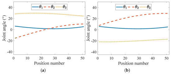
Figure 10.
IK solutions with different for each joint. (a) . (b) .
5.4. Manipulability Adjustment
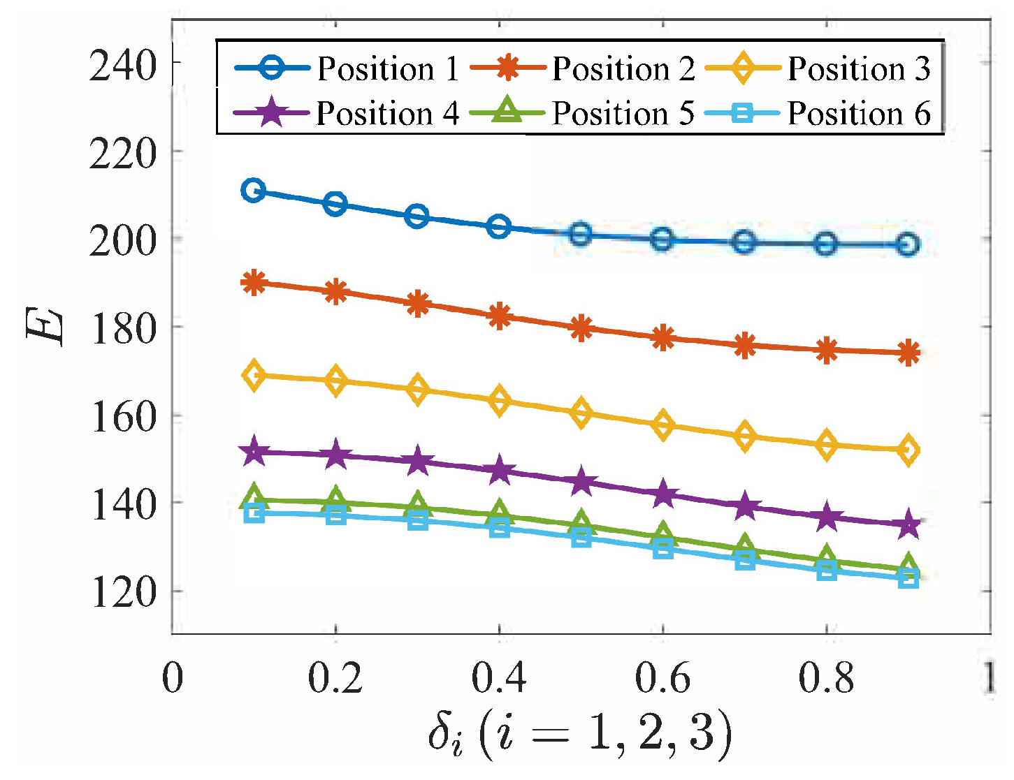
To investigate the impact of the adjustable IK solutions on the manipulability of the manipulator, we calculate the manipulability values corresponding to IK solutions under different for the same desired position. Table 5 lists six desired End-effector positions, which are obtained by specifying six different sets of joint angles and calculating the corresponding End-effector positions using the kinematics model, ensuring that all desired positions are within the manipulator’s workspace. Figure 11 illustrates the manipulability for these desired End-effector positions at different motion-level factors. It can be observed that for the same End-effector position, as increases, the manipulability of the corresponding manipulator configuration progressively decreases.
Table 5.
Desired End-effector positions.

Figure 11.
Manipulability of different motion-level factors .
6. Experimental Validations
6.1. Experimental Setup
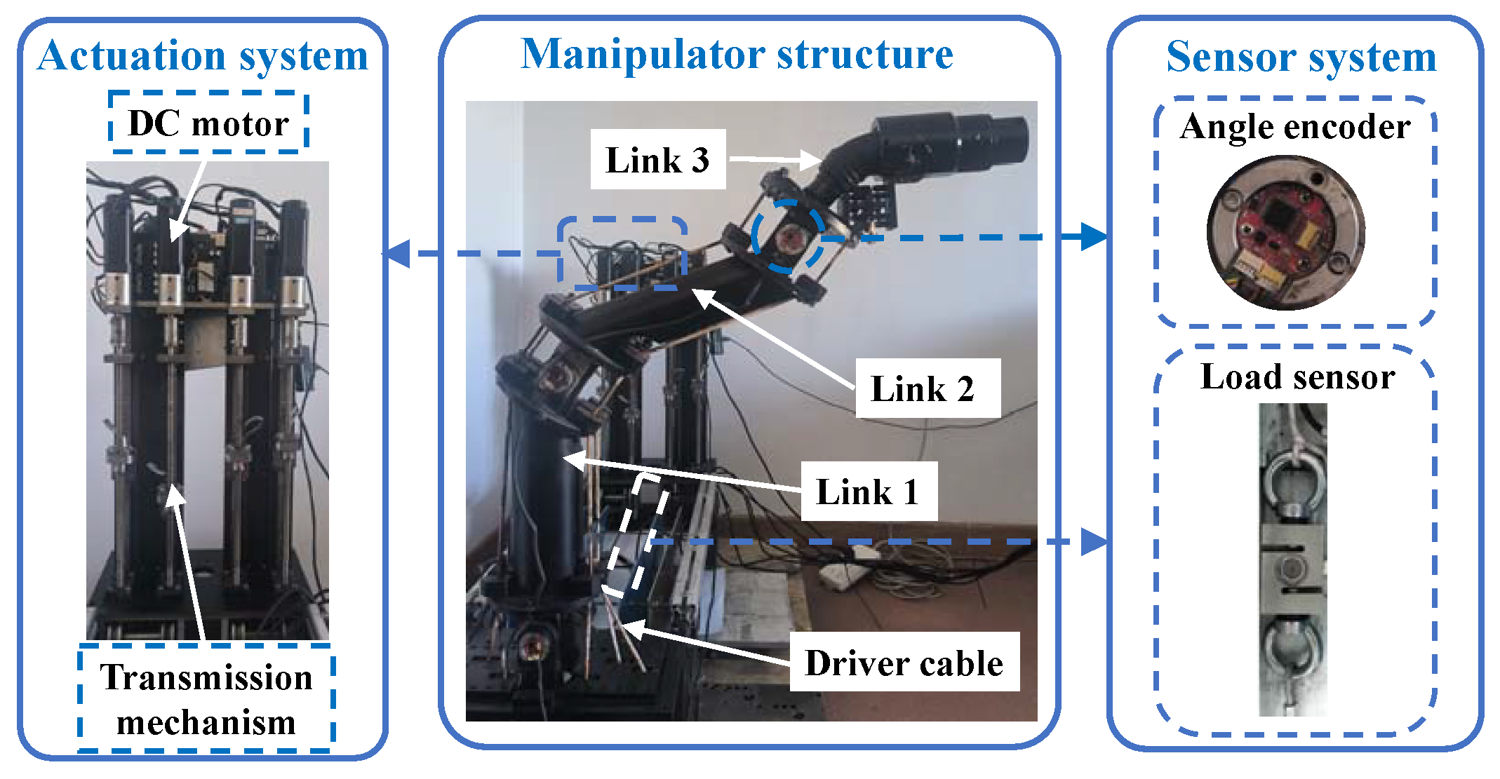
This section validates the effectiveness of the proposed method using a planar CDRM prototype. Figure 12 shows the experimental prototype, which consists of three links and three rotary joints and is driven by six cables. Motion control of the manipulator is achieved by adjusting the length and tension of the cables. Each cable is equipped with a tension sensor installed between the cable and the actuator to measure the cable tension. Additionally, each rotary joint is equipped with an encoder to measure its rotational angle. The experimental positions are measured using the forward kinematic model based on the joint angles obtained from the joint encoders. The precision of the angle encoders is , and the experimental position measurement accuracy is mm.
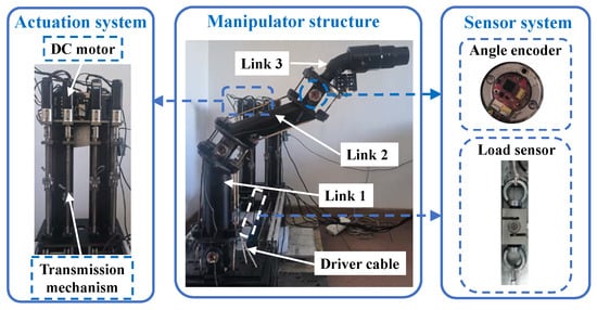
Figure 12.
Experimental prototype.
6.2. Adjustable IK Solutions Validation
To evaluate the difference between the experimental and desired positions, the error percentage of the experimental position relative to the desired position is calculated. This error percentage is defined as follows:
where and represent the experimental position and the desired position, respectively.
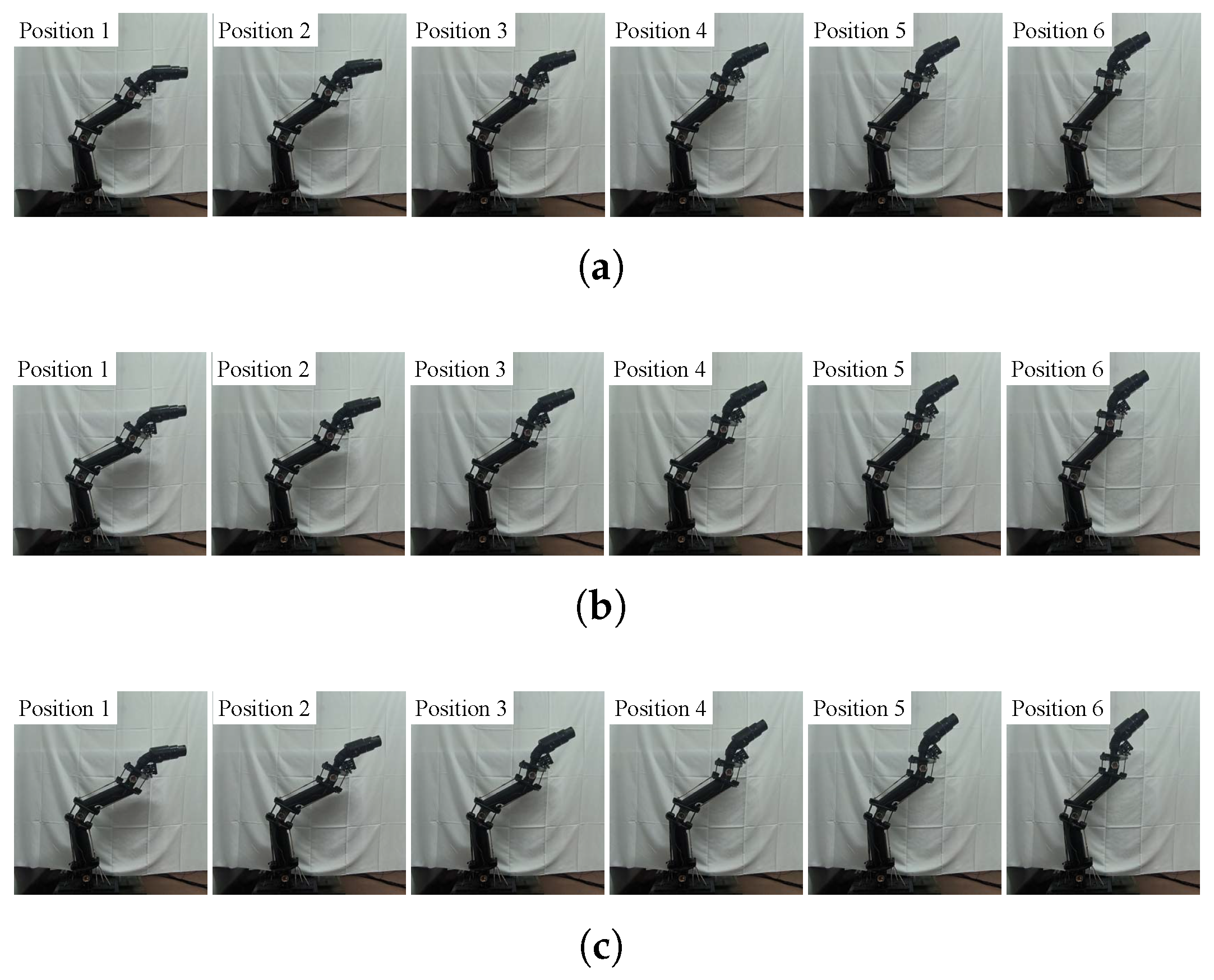
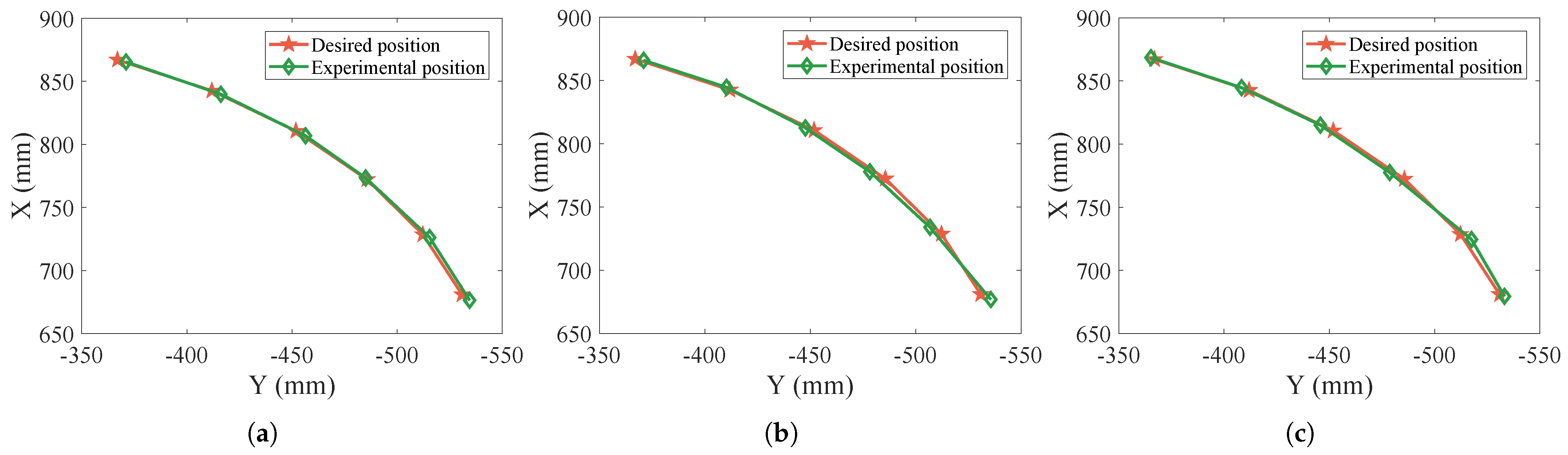
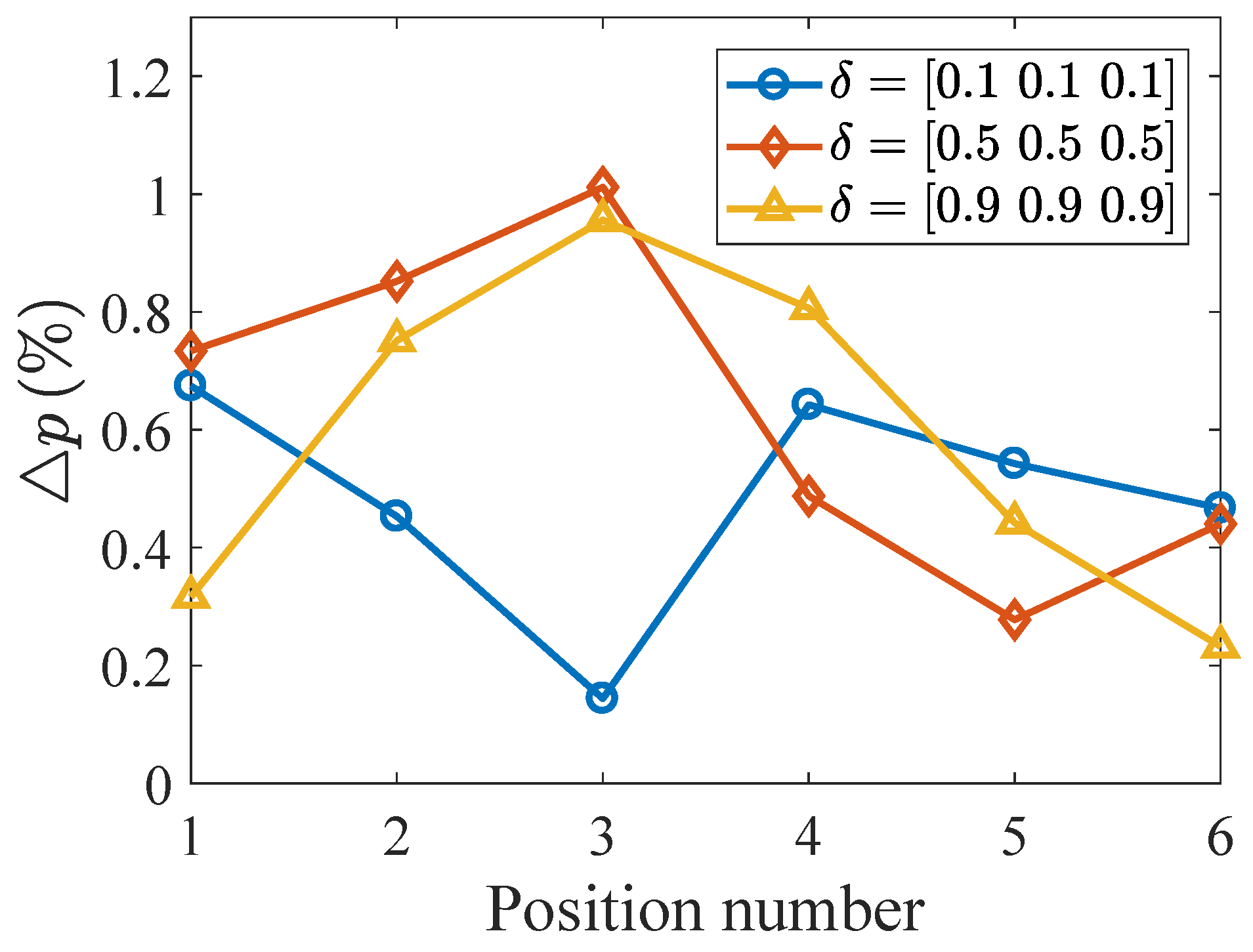
The experiments of adjustable IK solutions for the positions presented in Table 5 are shown in Figure 13. Table 6 presents the analytical and experimental IK solutions for motion-level factors of 0.1, 0.5, and 0.9. The comparison of the experimental results with the desired results is shown in Figure 14. Figure 15 illustrates the error percentage of the experimental positions relative to the desired positions. The maximum error percentage is , and the average error percentage is .
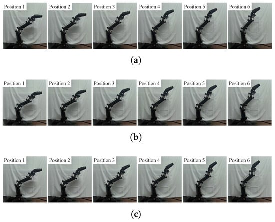
Figure 13.
Experimental positions of adjustable IK solutions under different motion-level factors. (a) . (b) . (c) .
Table 6.
IK solutions of desired End-effector positions.
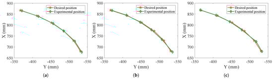
Figure 14.
Desired and experimental End-effector positions for three different motion-level factors. (a) . (b) . (c) .

Figure 15.
Error percentage of the experimental End-effector positions relative to the desired positions.
6.3. Manipulability Test
The error percentage of the experimental manipulability relative to the analytical manipulability is defined as follows:
where and represent the experimental manipulability and the analytical manipulability, respectively.
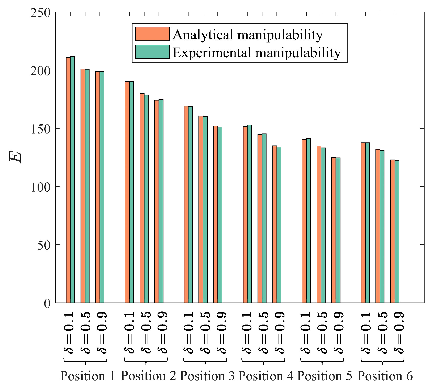
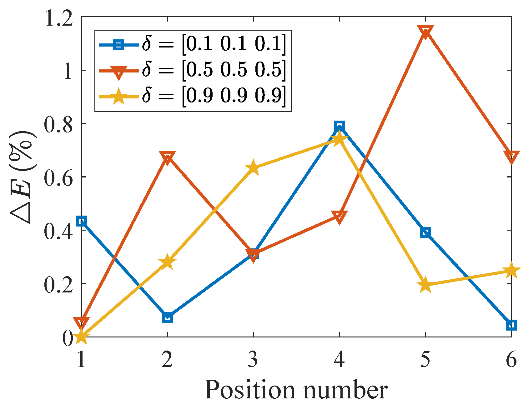
Figure 16 presents the analytical and experimental manipulability results. It is observed that the analytical and experimental results match closely. Figure 17 illustrates the error percentage of the experimental manipulability relative to the analytical manipulability. The maximum error percentage of the experimental manipulability relative to the analytical manipulability is , with an average error percentage of .
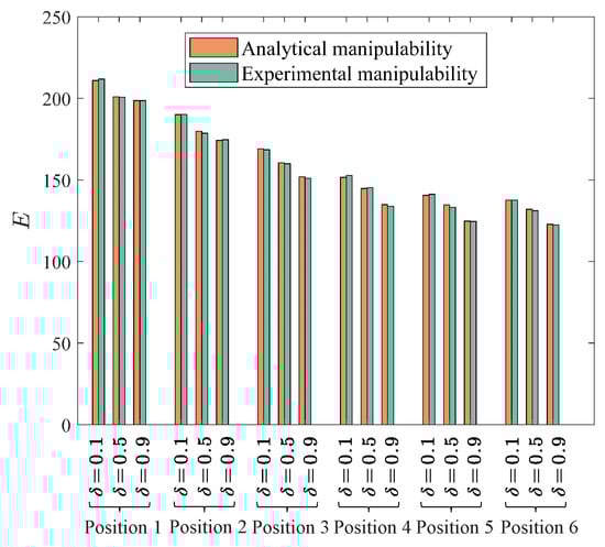
Figure 16.
Analytical and experimental manipulability results.
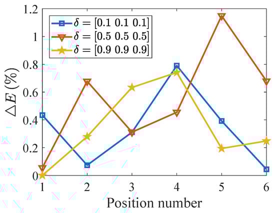
Figure 17.
Error percentage of the experimental manipulability relative to the analytical manipulability.
In summary, the experimental results are basically consistent with the analytical results, demonstrating the feasibility and effectiveness of the proposed method.
7. Conclusions
RMs often have an infinite number of feasible IK solutions for a given pose. This work presents an IK optimization method for RMs, aimed at obtaining adjustable IK solutions. By introducing the motion-level factor, we develop a performance metric for adjustable IK solutions. Adjusting the motion-level factor changes the position of the minimum value of the performance metric within the joint limits, thereby providing flexible control over the distribution of the IK solutions. A two-stage optimization algorithm is proposed to obtain adjustable IK solutions. In the first stage, a modified GPM is used to optimize the performance metric for the adjustable IK solutions, yielding the initial optimal solutions with the desired motion level. However, since the GPM introduces cumulative errors, the second stage employs the FABRIK algorithm to enhance accuracy, producing precise and optimal IK solutions while avoiding joint limits and singularity issues. Through simulations and experimental validation on a planar CDRM, the effectiveness of the proposed method is demonstrated. The IK solutions are successfully adjusted by modifying the motion-level factor, resulting in smooth and continuous solutions. Moreover, the manipulability of RMs can be regulated by adjusting the motion-level factor. This method provides an effective solution to the adjustable IK problem for RMs and is applicable to various types of RMs.
However, our method has certain limitations, such as the lack of experiments with a three-dimensional redundant manipulator. The method may demand substantial computational resources when addressing the inverse kinematics problem of a redundant manipulator with many DOFs, as it requires computing the pseudoinverse of the Jacobian matrix throughout the solution process. In future work, we plan to validate our method on three-dimensional redundant manipulators and further refine it. Additionally, adjustable inverse kinematics solutions can be leveraged to regulate the stiffness performance of redundant manipulators.
Author Contributions
Conceptualization, Z.L. and P.Q.; methodology, Z.L.; software, Z.L.; investigation, Z.L. and P.Q.; writing—original draft preparation, Z.L.; writing—review and editing, S.D. and Z.H. All authors have read and agreed to the published version of the manuscript.
Funding
This research received no external funding.
Institutional Review Board Statement
Not applicable.
Informed Consent Statement
Not applicable.
Data Availability Statement
The original contributions presented in this study are included in the article. Further inquiries can be directed to the corresponding author.
Conflicts of Interest
Author Zhiming Huang was employed by Shanghai Zhida Technology Development Co., Ltd. The remaining authors declare that the research was conducted in the absence of any commercial or financial relationships that could be construed as a potential conflict of interest.
Abbreviations
The following abbreviations are used in this manuscript:
| RM | Redundant manipulator |
| IK | Inverse kinematics |
| GPM | Gradient projection method |
| FABRIK | Forward and backward reaching inverse kinematics |
| TSOA | Two-stage optimization algorithm |
| DOF | Degree of freedom |
| LPM | Linear programming method |
| CDRM | Cable-driven redundant manipulator |
References
- Xu, X.T.; Xie, H.B.; Wang, C.; Yang, H.Y. Kinematic and dynamic models of hyper-redundant manipulator based on link eigenvectors. IEEE-ASME Trans. Mechatron. 2024, 29, 1306–1318. [Google Scholar] [CrossRef]
- Li, Y.; Wang, L. Kinematic model and redundant space analysis of 4-DOF redundant robot. Mathematics 2022, 10, 574. [Google Scholar] [CrossRef]
- Xu, H.; Xue, C.; Chen, Q.; Yang, J.; Liang, B. Continuous multi-target approaching control of hyper-redundant manipulators based on reinforcement learning. Mathematics 2024, 12, 3822. [Google Scholar] [CrossRef]
- Zhang, L.Y.; Gao, Y.M.; Mu, Z.G.; Yan, L.; Li, Z.X.; Gao, M.W. A variable stiffness planning method considering both the overall configuration and cable tension for hyper-redundant manipulators. IEEE-ASME Trans. Mechatron. 2024, 29, 659–667. [Google Scholar] [CrossRef]
- Xu, Z.H.; Li, S.A.; Zhou, X.F.; Zhou, S.B.; Cheng, T.B.; Guan, Y.S. Dynamic neural networks for motion-force control of redundant manipulators: An optimization perspective. IEEE Trans. Ind. Electron. 2021, 68, 1525–1536. [Google Scholar] [CrossRef]
- Peng, J.Q.; Xu, W.F.; Liu, T.L.; Yuan, H.; Liang, B. End-effector pose and arm-shape synchronous planning methods of a hyper-redundant manipulator for spacecraft repairing. Mech. Mach. Theory 2021, 155, 104062. [Google Scholar] [CrossRef]
- Endo, G.; Horigome, A.; Takata, A. Super dragon: A 10-m-long-coupled tendon-driven articulated manipulator. IEEE Robot. Autom. Lett. 2019, 4, 934–941. [Google Scholar] [CrossRef]
- Wang, M.F.; Dong, X.; Ba, W.M.; Mohammad, A.; Axinte, D.; Norton, A. Design, modelling and validation of a novel extra slender continuum robot for in-situ inspection and repair in aeroengine. Robot. Comput.-Integr. Manuf. 2021, 67, 102054. [Google Scholar] [CrossRef]
- Dong, X.; Axinte, D.; Palmer, D.; Cobos, S.; Raffles, M. Rabani, A.; Kell, J. Development of a slender continuum robotic system for on-wing inspection/repair of gas turbine engines. Robot. Comput.-Integr. Manuf. 2017, 44, 218–229. [Google Scholar] [CrossRef]
- Li, C.S.; Yan, Y.S.; Xiao, X.; Gu, X.Y.; Gao, H.X.; Duan, X.G.; Zuo, X.L.; Li, Y.Q.; Ren, H.L. A miniature manipulator with variable stiffness towards minimally invasive transluminal endoscopic surgery. IEEE Robot. Autom. Lett. 2021, 6, 5541–5548. [Google Scholar] [CrossRef]
- Kim, J.; Kwon, S.I.; Moon, Y.; Kim, K. Cable-movable rolling joint to expand workspace under high external load in a hyper-redundant manipulator. IEEE-ASME Trans. Mechatron. 2022, 27, 501–512. [Google Scholar] [CrossRef]
- Atawnih, A.; Papageorgiou, D.; Doulgeri, Z. Kinematic control of redundant robots with guaranteed joint limit avoidance. Robot. Auton. Syst. 2016, 79, 122–131. [Google Scholar] [CrossRef]
- Li, L.Y.; Gruver, W.A.; Zhang, Q.X.; Yang, Z.X. Kinematic control of redundant robots and the motion optimizability measure. IEEE Trans. Syst. Man Cybern. Part B-Cybern. 2001, 31, 155–160. [Google Scholar] [CrossRef]
- Zhang, Y.Y.; Li, S.; Kathy, S.; Liao, B.L. Recurrent neural network for kinematic control of redundant manipulators with periodic input disturbance and physical constraints. IEEE T. Cybern. 2019, 49, 4194–4205. [Google Scholar] [CrossRef]
- Qi, R.H.; Khajepour, A.; Melek, W.W. Redundancy resolution and disturbance rejection via torque optimization in hybrid cable-driven robots. IEEE Trans. Syst. Man Cybern.-Syst. 2021, 52, 4069–4079. [Google Scholar] [CrossRef]
- Yang, X.H.; Ma, B.Y.; Zhao, Z.Y.; Zhao, J.D.; Liu, H. A kinematics control scheme of redundant manipulators under unknown loads or external forces. IEEE Trans. Syst. Man Cybern.-Syst. 2024, 54, 5048–5060. [Google Scholar] [CrossRef]
- Jin, L.; Li, S.; La, H.M.; Luo, X. Manipulability optimization of redundant manipulators using dynamic neural networks. IEEE Trans. Ind. Electron. 2017, 64, 4710–4720. [Google Scholar] [CrossRef]
- Yang, X.H.; Zhao, Z.Y.; Ma, B.Y.; Xu, Z.C.; Zhao, J.D.; Liu, H. Kinematic and dynamic manipulability optimizations of redundant manipulators based on RNN model. IEEE Trans. Ind. Inform. 2024, 20, 5763–5773. [Google Scholar] [CrossRef]
- Park, K.C.; Chang, P.H.; Lee, S. A new kind of singularity in redundant manipulation: Semi algorithmic singularity. In Proceedings of the 19th IEEE International Conference on Robotics and Automation (ICRA), Washington, DC, USA, 11–15 May 2002; pp. 1979–1984. [Google Scholar]
- Liegeois, A. Automatic supervisory control of the configuration and behavior of multibody mechanisms. IEEE Trans. Syst. Man Cybern. 1977, 7, 868–871. [Google Scholar]
- Zghal, H.; Dubey, R.V.; Euler, J.A. Efficient gradient projection optimization for manipulators with multiple degrees of redundancy. In Proceedings of the IEEE International Conference on Robotics and Automation, Cincinnati, OH, USA, 13–18 May 1990; Volume 2, pp. 1006–1011. [Google Scholar]
- Chan, T.F.; Dubey, R.V. A weighted least-norm solution based scheme for avoiding joint limits for redundant joint manipulators. IEEE Trans. Robot. Autom. 1995, 11, 286–292. [Google Scholar] [CrossRef]
- Xiang, J.; Zhong, C.W.; Wei, W. General-weighted least-norm control for redundant manipulators. IEEE Trans. Robot. 2010, 26, 660–669. [Google Scholar] [CrossRef]
- Wan, J.; Wu, H.T.; Ma, R.; Zhang, L.A. A study on avoiding joint limits for inverse kinematics of redundant manipulators using improved clamping weighted least-norm method. J. Mech. Sci. Technol. 2018, 32, 1367–1378. [Google Scholar] [CrossRef]
- Dubey, R.V.; Euler, J.A.; Babcock, S.M. An efficient gradient projection optimization scheme for a seven-degree-of-freedom redundant robot with spherical wrist. In Proceedings of the 1988 IEEE International Conference on Robotics and Automation, Philadelphia, PA, USA, 24–29 April 1988; Volume 1, pp. 28–36. [Google Scholar]
- Dubey, R.V.; Euler, J.A.; Babcock, S.M. Real-time implementation of an optimization scheme for 7-degrees-of-freedom redundant manipulators. IEEE Trans. Robot. Autom. 1991, 7, 579–588. [Google Scholar] [CrossRef]
- Zhang, X.L.; Fan, B.H.; Wang, C.J.; Cheng, X.L. An improved weighted gradient projection method for inverse kinematics of redundant surgical manipulators. Sensors 2021, 21, 7362. [Google Scholar] [CrossRef] [PubMed]
- Shimizu, M.; Kakuya, H.; Yoon, W.K.; Kitagaki, K.; Kosuge, K. Analytical inverse kinematic computation for 7-DOF redundant manipulators with joint limits and its application to redundancy resolution. IEEE Trans. Robot. 2008, 24, 1131–1142. [Google Scholar] [CrossRef]
- Faria, C.; Ferreira, F.; Erlhagen, W.; Monteiro, S.; Bicho, E. Position-based kinematics for 7-DoF serial manipulators with global configuration control, joint limit and singularity avoidance. Mech. Mach. Theory 2018, 121, 317–334. [Google Scholar] [CrossRef]
- Li, Z.J.; Brandstötter, M.; Hofbaur, M. Kinematic redundancy analysis for (2n+1) R circular manipulators. IEEE Trans. Robot. 2023, 39, 755–767. [Google Scholar] [CrossRef]
- Aristidou, A.; Lasenby, J. FABRIK: A fast, iterative solver for the Inverse Kinematics problem. Graph. Model. 2011, 73, 243–260. [Google Scholar] [CrossRef]
- Liu, T.L.; Yang, T.W.; Xu, W.F.; Mylonas, G.; Liang, B. Efficient inverse kinematics and planning of a hybrid active and passive cable-driven segmented manipulator. IEEE Trans. Syst. Man Cybern.-Syst. 2022, 52, 4233–4246. [Google Scholar] [CrossRef]
- Kolpashchikov, D.Y.; Laptev, N.V.; Danilov, V.V.; Skirnevskiy, I.P.; Manakov, R.A.; Gerget, O.M. FABRIK-based inverse kinematics for multi-section continuum robots. In Proceedings of the 18th International Conference on Mechatronics - Mechatronika (ME), Brno, Czech Republic, 5–7 December 2018; pp. 288–295. [Google Scholar]
- Zhang, W.H.; Yang, Z.X.; Dong, T.L.; Xu, K. FABRIKc: An efficient iterative inverse kinematics solver for continuum robots. In Proceedings of the 2018 IEEE/ASME International Conference on Advanced Intelligent Mechatronics (AIM), Auckland, New Zealand, 9–12 July 2018; pp. 346–352. [Google Scholar]
- Yoshikawa, T. Manipulability of robotic mechanisms. Int. J. Robot. Res. 1985, 4, 3–9. [Google Scholar] [CrossRef]
Disclaimer/Publisher’s Note: The statements, opinions and data contained in all publications are solely those of the individual author(s) and contributor(s) and not of MDPI and/or the editor(s). MDPI and/or the editor(s) disclaim responsibility for any injury to people or property resulting from any ideas, methods, instructions or products referred to in the content. |
© 2025 by the authors. Licensee MDPI, Basel, Switzerland. This article is an open access article distributed under the terms and conditions of the Creative Commons Attribution (CC BY) license (https://creativecommons.org/licenses/by/4.0/).