Signal Detection for Enhanced Spatial Modulation-Based Communication: A Block Deep Neural Network Approach

Abstract

As a novel variant of spatial modulation (SM), enhanced SM (ESM) provides higher spectral efficiency and improved bit error rate (BER) performance compared to SM. In ESM, traditional signal detection methods such as maximum likelihood (ML) have the drawback of high complexity. Therefore, in this paper, we try to solve this problem using a deep neural network (DNN). Specifically, we propose a block DNN (B-DNN) structure, in which smaller B-DNNs are utilized to identify the active antennas along with the constellation symbols they transmit. Simulation outcomes indicate that the BER performance related to the introduced B-DNN method outperforms both the minimum mean-square error (MMSE) and the zero-forcing (ZF) methods, approaching that of the ML method. Furthermore, the proposed method requires less computation time compared to the ML method.

1. Introduction

Multiple-input multiple-output (MIMO) is a widely used technology in current wireless communication systems, which can improve data transmission rate and increase channel capacity. But this technology also faces some practical issues such as inter-channel interference (ICI) and inter-antenna synchronization (IAS). Consequently, to solve these problems, spatial modulation (SM) was proposed in [1]. In terms of SM, at any given time slot, only one antenna is active, and a specific number of information bits are mapped to the index part and the constellation part, where the index part is used to select the activated antenna while the constellation part decides the constellation symbol.

However, SM only has one activated antenna at each time slot, which results in a low data rate. Hence, to solve this issue, enhanced SM (ESM) was proposed in [2]. ESM takes into account more than one signal constellation to increase the combination of antennas and symbols. When only one antenna is activated, that single antenna transmits symbols from the primary constellation. When two antennas are activated, both antennas simultaneously transmit symbols from the secondary constellation. In comparison to SM, it enhances spectral efficiency and achieves a lower bit error rate (BER), showing significant potential for future applications.

Deep neural network (DNN) has made profound inroads in the wireless communications, manifesting its prowess in diverse applications such as channel coding [3], antenna selection [4] and modulation classification [5] as well as other applications [6,7,8,9]. Recently, several extensions of DNN research achieved notable results. Several researchers have improved the structure of neural networks, leading to the development of more powerful networks, such as Kolmogorov–Arnold networks (KAN) [10]. Other researchers focus on integrating DNN with other technologies to enhance their performance in complex tasks, such as cognitive computing [11]. These efforts can refine and expand the applications of DNN in wireless communications, representing a promising direction for future research. At the same time, KAN and cognitive computing also have some applications in wireless communications. For instance, cognitive computing can be employed to predict the flow status of rectifiers, allowing for preemptive adjustments of network parameters and optimized power management. Moreover, cognitive computing can be utilized for real-time monitoring and analysis of communication signal characteristics, thereby optimizing signal processing algorithms. In terms of KAN, as a recent development in deep learning, it can be used to predict the performance of flexible electrohydrodynamic (EHD) pumps, which in turn can optimize the allocation of network resources. In terms of signal detection, several investigations have been conducted to improve the detection accuracy and complexity problem. In these works, some researchers attempt to improve the structure of neural network in order to enhance the performance of such neural networks in applications related to wireless communications [12,13,14]. If we consider the use of SM, in [15], the author used a block deep neural network (B-DNN) for signal detection in generalized SM (GSM). Experimental results showed that the B-DNN could approach the performance of the maximum likelihood (ML) method in terms of BER while exhibiting lower complexity. In [16], the author considered the use of neural network-assisted partial detection in GSM, with one neural network module for detecting the antenna index and another for detecting the received constellation symbol. This approach further reduced complexity. Authors in [17,18] explored the possibility of using DNN for signal detection in quadrature SM (QSM) and the results demonstrated the feasibility of DNN. Previous work has demonstrated that employing DNN for signal detection in GSM and QSM can reduce complexity while maintaining a low BER. In ESM, as a new variant of SM, to the best of our knowledge, the DNN method for signal detection in ESM has not yet been utilized.

In order to fill this gap, we propose a B-DNN method for signal detection in ESM. As an improved version of DNN, the B-DNN has already demonstrated its superior performance in signal detection for GSM. The B-DNN detector is capable of achieving a lower BER compared to the two linear detectors, minimum mean-square error (MMSE) and zero-forcing (ZF). In addition, it approaches the optimal BER performance of the ML detector while maintaining lower complexity and computational time. Moreover, compared to conventional DNN, the B-DNN shows improvements in both training time and accuracy. Furthermore, when compared to other well-known neural networks, such as convolutional neural network (CNN), the B-DNN exhibits better BER performance, with specific numerical results provided in [15]. Building on these findings, we apply this B-DNN to ESM to demonstrate whether this neural network architecture continues to perform well in another form of SM. In the data pre-processing phase, we utilize a feature vector generator (FVG) to transform complex in-phase and quadrature (IQ) data into a pure format, enhancing the performance in the symbol classification phase. During the training phase, we design a feed-forward neural network, which is meticulously trained on input vectors from the data pre-processing phase. The output of the neural network is classified using the softmax function, renowned for its efficacy in differentiating between multiple classes. The simulation results from our experiments clearly demonstrate that the B-DNN-based detector not only accurately approximates the ML detector but also significantly outperforms the traditional MMSE and ZF detectors in terms of BER. Moreover, B-DNN based detector can also reduce the classification time compared to ML detector, which greatly enhances the efficiency of the detection process, highlighting its potential for practical applications in ESM systems.

2. ESM System Model and Conventional Detectors

2.1. MIMO System Model

In MIMO system operating over quasi-static flat fading channel, the received signal is expressed as follows:

$$\mathbf{y}=\mathbf{H}\mathbf{x}+\mathbf{n},$$

(1)

where $\mathbf{H}\in {\mathbb{C}}^{N_r\times N_t}$ denotes a channel matrix that follows a complex Gaussian distribution $\mathcal{CN}(\mathbf{0},\mathbf{1})$ with $N_r$ representing the number of antennas at the receiver and $N_t$ representing the number of antennas at the transmitter. $\mathbf{x}\in {\mathbb{C}}^{N_p\times 1}$ is the transmitted signal vector. In ESM, when $N_p$ equals to 1, the primary constellation is used, and when $N_p$ equals to 2, the secondary constellation is used. The details of this mechanism are introduced in the next section. And the Gaussian noise $\mathbf{n}$ follows the distribution of $\mathcal{CN}(\mathbf{0},{\sigma }^2\mathbf{I})$, where $\mathbf{I}$ means identity matrix and $\sigma$ is the variance of the noise and the size of this parameter is ${\mathbb{C}}^{N_r\times 1}$.

2.2. ESM System Framework

In this paper, we consider the case of two transmit antennas (2-TX) in the ESM system, and the primary modulation is quadrature phase shift keying (QPSK). Based on the above, the transmitted vector set $\mathbf{X}$ can be represented as

$$\mathbf{X}\in \{[\begin{array}{c}{\mathcal{C}}_4\\ 0\end{array}],[\begin{array}{c}0\\ {\mathcal{C}}_4\end{array}],[\begin{array}{c}{\mathcal{B}}_2^0\\ {\mathcal{B}}_2^0\end{array}],[\begin{array}{c}{\mathcal{B}}_2^1\\ {\mathcal{B}}_2^1\end{array}]\},$$

(2)

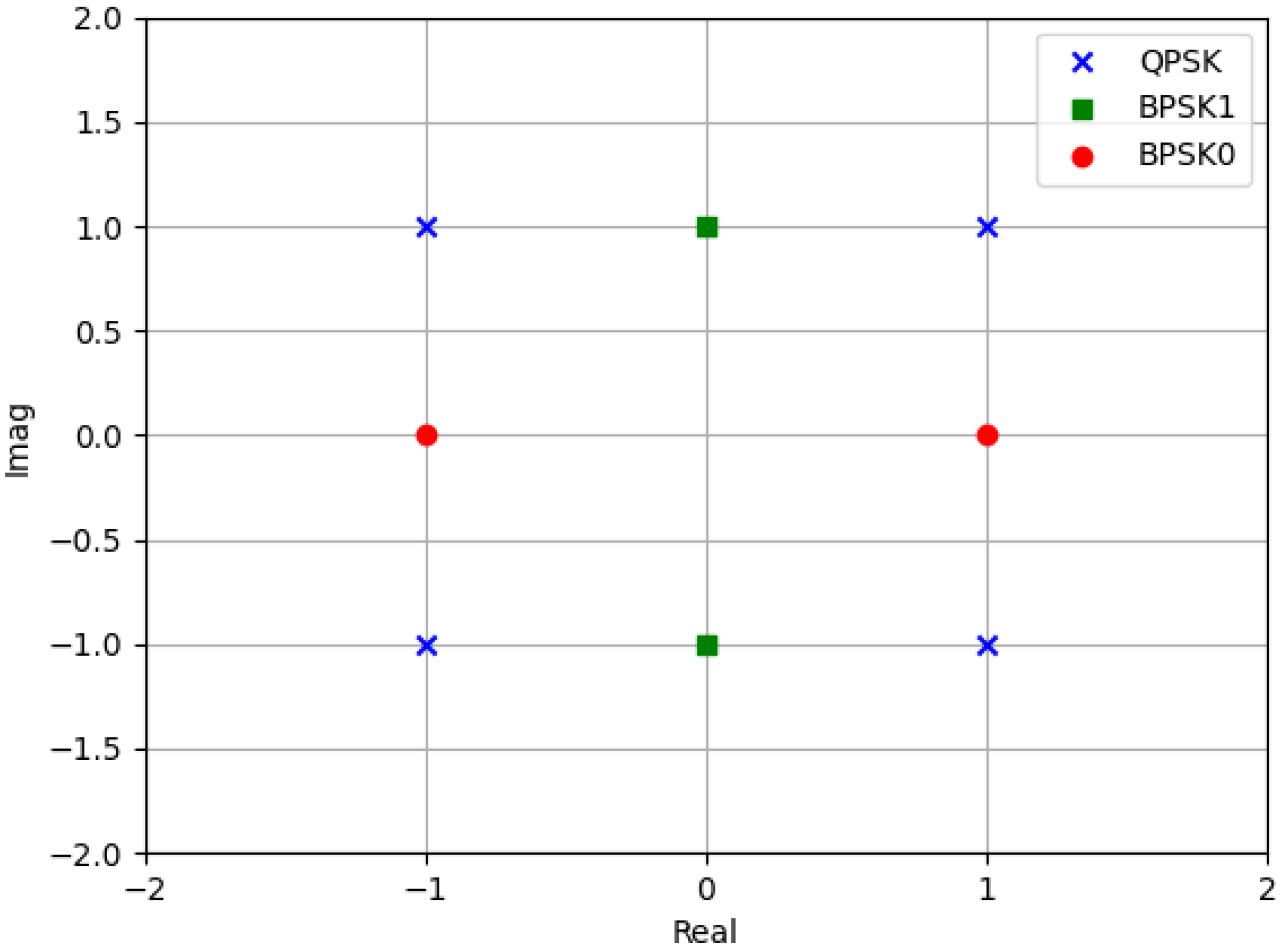
where ${\mathcal{C}}_4$ denotes the QPSK signal constellation used as the primary constellation and ${\mathcal{B}}_2^0$, ${\mathcal{B}}_2^1$ represent two secondary constellations given by ${\mathcal{B}}_2^0$ = $\{+1,-1\}$, ${\mathcal{B}}_2^1$ = $\{+i,-i\}$. Clearly, the first two components of the transmission vector correspond to the scenario where a single antenna is activated, transmitting a symbol from the primary constellation. The last two components correspond to a scenario where two antennas are activated, and both transmission antennas can simultaneously transmit symbols from the secondary constellation. However, each of these symbols carries only 1 bit of information, which is half the amount carried by the symbols from the primary constellation. The goal of this approach is to match the bit quantity conveyed by the first and second components. Additionally, the derivation of the secondary constellation is primarily guided by the criterion of maximizing the minimum Euclidean distance between the primary and secondary constellations without increasing the transmitted signal power. We name ${\mathcal{B}}_2^0$ as Binary Space Shift Keying 0 (BPSK0) and ${\mathcal{B}}_2^1$ as Binary Space Shift Keying 1 (BPSK1). An example of the signal constellation implemented for this design can be observed in Figure 1, where four signal space elements are described in Table 1. In each time slot, the number of activated antennas is $Np$ and this scheme transmits 4 bits per channel use (bpcu). The number of bits of information is divided into two parts, where one part is used for the selection of transmit antenna combinations (TACs), and the other part is used for carrying symbol bits. Based on this, the number of bits for TAC ($B-TAC$) and symbol ($B-SYM$) can be expressed as

$$B-TAC={log}_{2}TAC,$$

(3)

$$B-SYM=N_p{log}_{2}M,$$

(4)

where the values of $N_p$ and M depend on primary constellation and secondary constellation. Since we have $N_p$ activated antennas, we can represent the transmitted signal vectors $\mathbf{x}$ by

$$\mathbf{x}={[s_1,s_2,s_3,\dots ,s_{Np-1},0,s_{N_p},\dots ,0]}^T,$$

(5)

with symbols $s_1,s_2,s_3,\dots \dots ,s_{N_{p-1}},s_{N_p}\in \mathbb{S}$, and $\mathbb{S}$ is the constellation collection which includes all the symbols in Figure 1.

Figure 1. An illustration of the constellations used. The crosses represent QPSK, the circles represent BPSK0 and the squares represent BPSK1 signal constellation.

Table 1. Enhanced SM, 2TX-4 bpcu.

	Tx1	Tx2
C1	QPSK	0
C2	0	QPSK
C3	BPSK0	BPSK0
C4	BPSK1	BPSK1

2.3. Conventional Detection

2.3.1. ML Detector Scheme

ML detection has the best BER performance, and it can be formulated as

$$\left(\widehat{\mathit{s}}\right)=arg\underset{\mathit{s}\in \mathbb{S}}{min}\left|\right|\mathbf{y}-{\mathbf{H}s\left|\right|}_F^2,$$

(6)

which performs a comprehensive search of potential transmitted signal vectors to concurrently identify the activated antennas and constellation points, resulting in a substantial increase in decoding complexity of the receiver. This exhaustive methodology, while ensuring optimal detection accuracy, requires considerable computational resources.

2.3.2. Conventional Detect Method

As the number of transmit antennas and modulation levels increases, the complexity of the ML algorithm escalates exponentially. Therefore, several computational efficient algorithms such as ZF and MMSE are also employed and tested in this paper. The formulation for the ZF detection approach is provided in the subsequent equation:

$${\widehat{\mathbf{x}}}_{ZF}={\mathbf{H}}^H\mathbf{y}{\left({\mathbf{H}}^H\mathbf{H}\right)}^{-1},$$

(7)

where the conjugate transpose of matrix $\mathbf{H}$ can be represented as ${\mathbf{H}}^H$. This method is sensitive to channel noise, which limits its performance in the presence of strong noise effects. From this perspective, the MMSE method, which takes noise into account, yields better BER performance than ZF. The MMSE expression is as follows:

$${\widehat{\mathbf{x}}}_{MMSE}={({\mathbf{H}}^H\mathbf{H}+{\sigma }^2\mathbf{I})}^{-1}{\mathbf{H}}^H\mathbf{y}.$$

(8)

MMSE detection takes into account the impact of noise during the equalization process, but in doing so, the noise may be amplified, especially when the channel conditions are poor. Therefore, MMSE detection requires a higher degree of accuracy in channel state information (CSI), and from this perspective, the difficulty of implementing MMSE is greater.

3. Proposed ESM Block-DNN Detector

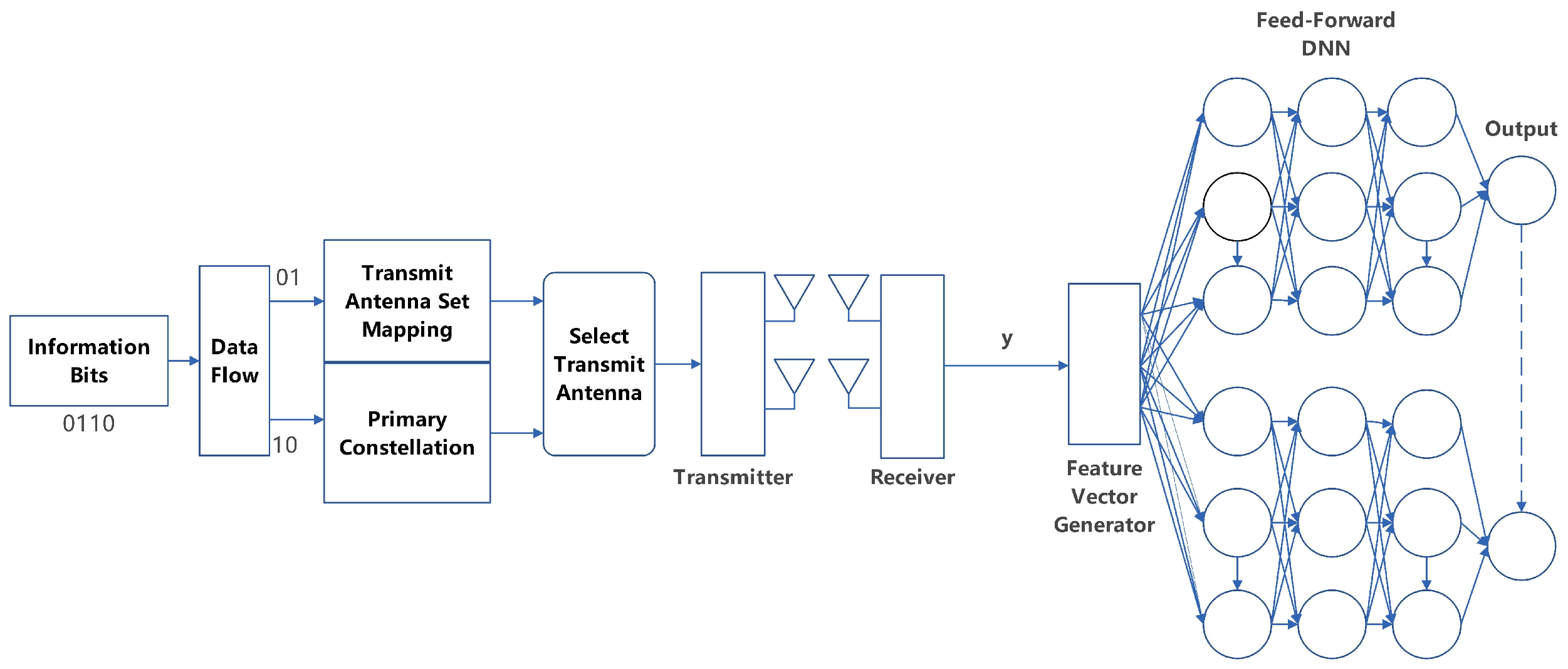
In this section, we elucidate the working principle of the proposed detection mechanism. Figure 2 illustrates the framework of the ESM detector when one antenna is activated and sends QPSK signal. Regarding the secondary constellation, the constellation part only needs to be adjusted to two antennas sending the same BPSK0 or BPSK1 signal simultaneously. In order to enhance the precision of the B-DNN detector, we train separate neural networks for each case of ESM-2TX presented in Table 1. The main parameters are given in Table 2. Comparing with traditional DNN, we use a smaller B-DNN to detect the number of antennas activated by each case and the corresponding constellation symbols. In order to build the B-DNN, three distinct steps are required: data pre-processing, training and prediction.

Figure 2. Diagram of ESM communication system with DNN signal detection.

Table 2. Significant Parameters in DNN.

	Tx1
Input nodes	2($N_r{N}_p+N_r$)
Learning rate	0.005
Hidden layer	3
Number of training set	15,000,000
Output nodes	M
Number of validation set	5,000,000
Hidden layer activation	ReLu
Epoch	50
Output layer activation	Softmax
Loss function	Cross-entropy
QPSK hidden nodes	256-128-64
BPSK0 hidden nodes	256-128-64
BPSK1 hidden nodes	256-128-64
Optimizer	SGD

3.1. Data Pre-Processing

According to [19], in the realm of neural networks, the efficacy of data pre-processing is paramount in ensuring the excellence of outcomes. Data pre-processing is an essential preliminary step that involves the meticulous refinement of raw data before they are imported to the neural network for training. This process includes data purification.

3.1.1. Raw Data

According to Equation (1), signal vector $\mathbf{y}$ is the sum of signals received from $N_r$ antennas. Concurrently, we hold four distinct combinations. In the scenario where only one antenna is activated, we use column vectors from the channel matrix $\mathbf{H}$. In the other scenario, the entire channel matrix $\mathbf{H}$ is used as the input vector.

3.1.2. Feature Vector Generator

Given that the raw data consist of multiple matrices containing complex-valued IQ components, it is crucial to convert them into vector form. In this pivotal phase, we employ a sophisticated technique called separated FVG (SFVG) to handle raw data. The quintessence of SFVG lies in its capability to decompose the complex-valued IQ data into real-valued vector components. For instance, we input channel matrix $\mathbf{H}$ into SFVG and the output is given by the following expression:

$$\begin{array}{c}{\mathbf{f}}_{SFVG}\left(\mathbf{H}\right)=\left[\right|\mathfrak{R}\left(h_{1,1}\right)|,|\mathfrak{I}\left(h_{1,1}\right)|\\ ,|\mathfrak{R}\left(h_{1,2}\right)|,|\mathfrak{I}\left(h_{1,2}\right)|\\ ,\dots ,|\mathfrak{R}\left(h_{u,o}\right)|,|\mathfrak{I}\left(h_{u,o}\right)|\\ ,\dots ,|\mathfrak{R}\left(h_{N_r,N_t}\right)|,|\mathfrak{I}\left(h_{N_r,N_t}\right){\left|\right]}^T.\end{array}$$

(9)

3.1.3. Expression of the Training Input

Upon obtaining the output of SFVG, we denote ${\mathbf{D}}^j$ = $[{\mathbf{d}}_1,\dots ,{\mathbf{d}}_i,\dots ,{\mathbf{d}}_N]$ as the jth element of the N-dimensional training dataset input, where j ranges over $\{1,2,\dots ,N_s\}$, signifying the time slot index of the data. Given the original datasets that consist of N combinations of active antennas from the column of the channel matrix ${\mathbf{H}}_I$ and the received signal vector y, ${\mathbf{d}}_i$ can be expressed as

$${\mathbf{d}}_i={[{\mathbf{f}}_{SFVG}{\left({\mathbf{y}}_j\right)}^T,{\mathbf{f}}_{SFVG}{\left({\mathbf{H}}_{I_i}^{\left(j\right)}\right)}^T]}^T,$$

(10)

where ${\mathbf{d}}_i\in {\mathbb{R}}^{(2N_r+2N_r{N}_p)\times 1}.$

3.2. B-DNN Parameters and Training

An array of L fully connected neural layers, including L–1 hidden layers, is designed to decode the signals emanating from each active transmit antenna at the transmitter. Table 2 delineates the parameters of the proposed DNN, including the count of layers, where the lth layer is endowed with ${\delta }_l$ nodes.

We use $\lambda$ to represent the comprehensive collection of parameters within the DNN, where $\lambda$ is defined as $\lambda =\{{\lambda }_1,{\lambda }_2,\dots ,{\lambda }_L\}$. The parameters specific to the lth layer are signified by ${\lambda }_l=\{{\mathbf{W}}^l,{\mathbf{b}}_l\}$. Consequently, the lth layer is delineated as

$${\mathbf{Z}}_l=\sigma ({\mathbf{W}}^l{\mathbf{Z}}_{l-1}+{\mathbf{b}}_l),$$

(11)

where the weight matrix can be expressed as ${\mathbf{W}}^l\in {\mathbb{R}}^{{\delta }^{l-1}\times {\delta }_l}$ and the deviation vector ${\mathbf{b}}_l\in {\mathbb{R}}^{{\delta }_l\times 1}$, $\sigma (·)$ is the activation function. Apart from the final layer, the end of each layer uses a famous method, called Rectified linear unit (ReLU), and the expression is $\sigma \left(x\right)=max(0,x)$. The derivative of this method consistently yields a singular value, oscillating between the binary states of zero and one, thereby preventing the exponential diminution of gradient magnitude as it traverses the depth of numerous layers. The ReLU function facilitates rapid learning within the DNN. This in turn renders the efficient training of a profound supervised network feasible, obviating the need for unsupervised pre-training, as elucidated in [20]. In the penultimate layer, we employ the renowned softmax function to map the output onto a continuum that spans the interval $\left[0,1\right]$, and the mapping of the input and output of the DNN can be represented by the following equation:

$$\begin{array}{cc}\hfill {\mathbf{Z}}_L& =\sigma ({\mathbf{W}}^{\left(L\right)}\left(\sigma \right({\mathbf{W}}^{(L-1)}(\dots \sigma \left({\mathbf{W}}^{\left(1\right)}{\mathbf{Z}}_0+{\mathbf{b}}_1\right)\dots )\hfill \\ & +{\mathbf{b}}_{L-1}\left)\right)+{\mathbf{b}}_L\left)\right).\hfill \end{array}$$

(12)

We utilize categorical cross-entropy to ascertain the discrepancy in the cost function between the actual data and the predicted outcomes, thereby facilitating the identification of parameters that enhance our network’s optimization. We let ${\mathbf{Z}}_T$ represent the one-hot encoded vector signifying the labels for the supervised training phase, which contrasts with the output of the predictions, denoted as ${\mathbf{Z}}_L$. The expression for this method is given as follows:

$$\widehat{L}({\mathbf{Z}}_T,{\mathbf{Z}}_L)=-\sum _{n=1}^M{Z}_{T_n}log\left(Z_{L_n}\right),$$

(13)

where the difference between $Z_{T_n}$ and $Z_{L_n}$ should be minimized. The objective is to effectuate its reduction to the greatest extent possible. To achieve this, we employ the stochastic gradient descent (SGD) optimization technique. This process involves the strategic adjustment of the existing weight values by either incrementing or decrementing them in accordance with the gradient’s magnitude, modulated by the learning rate, thus facilitating an efficient traversal towards the minimum of the optimization target. The parameter $\eta$, known as the learning rate, is a crucial hyper-parameter that is constrained to the interval from zero to one. It plays a significant role in the SGD algorithm, which incrementally refines the parameters over iterations through the application of gradient information. The following equation illustrates this process of updating the parameters:

$${\mathbf{W}}_{t+1}^{\left(l\right)}={\mathbf{W}}_t^{\left(l\right)}-\eta {\displaystyle \frac{\partial \widehat{L}({\mathbf{Z}}_T,{\mathbf{Z}}_L)}{\partial {\mathbf{W}}_t^{\left(l\right)}}}.$$

(14)

The iterative refinement of weights persists in a cyclical fashion until the cost function’s value indicates a state of equilibrium over successive iterations. Upon attaining the optimal set of weights, the capability to make predictions is enabled through the utilization of the trained feed-forward DNN.

Throughout the training phase, it is essential to have the input vectors for training and their corresponding tags. The input vectors for training are derived from the channel matrix $\mathbf{H}$ as well as the received signal vector $\mathbf{y}$, which could be formulated as ${\mathbf{d}}_i={[{\mathbf{f}}_{SFVG}{\left({\mathbf{y}}_j\right)}^T,{\mathbf{f}}_{SFVG}{\left({\mathbf{H}}_{I_i}^j\right)}^T]}^T$. For the tags, a one-hot encoding scheme is implemented, creating a vector of length M that corresponds to the transmitted symbol. This vector represents the M-PSK symbol constellation, thereby providing a distinct label for each point in the constellation.

At the same time, during the training phase, certain issues often arise, such as overfitting. To mitigate the impact of this problem, we implement several strategies. Firstly, we employ L2 regularization, which imposes a penalty on the sum of the squares of the weights, preventing them from becoming excessively large. This helps to reduce the complexity of the model and prevent overfitting. The regularization coefficient is set to 0.001 during the training phase. Additionally, batch normalization is incorporated after the hidden layers; this technique normalizes the features of each mini-batch to have a mean of zero and a variance of one. Furthermore, dropout is introduced at the end of the hidden layers, which randomly sets a proportion of neurons and their connections to zero with a certain probability. This prevents neurons within the network from becoming overly reliant on specific features, thereby encouraging the network to learn more robust and generalized feature representations. These strategies can significantly reduce the effects of overfitting.

3.3. Prediction Phase

After completing the aforementioned tasks, we begin to use this well-trained model for predictions. We possess N input vectors ${\mathbf{d}}_n$ within the jth time slot of predictive phase and each of these vectors engenders $N_p$ output vectors. These output vectors, denoted as ${\mathbf{Z}}_L$, belong to the positive real space ${\mathbb{R}}_{+}^{M\times 1}$ and correspond to the k-th active antenna. Subsequently, the prediction of the transmitted symbol ${\widehat{s}}_{i_k}={\mathcal{S}}_n$ and $\widehat{n}$ can be secured and expressed as the following formula:

$$\left(\widehat{n}\right)=\underset{n\in \{1,\dots ,M\}}{argmax}\left({{\mathbf{Z}}_L}_n\right).$$

(15)

Identifying the result through calculating the Euclidean distance between the received symbol and the estimated symbol is given in the expression of

$$\left(\widehat{i}\right)=arg\underset{i\in \{1,\dots ,N\}}{min}{∥{\mathbf{y}}^{\left(j\right)}-\sqrt{E_s}{\mathbf{H}}_{Ii}^{\left(j\right)}{\widehat{\mathbf{s}}}_i^{\left(j\right)}∥}_F^2,$$

(16)

Through utilizing the smallest index $\widehat{i}$, we proceed to perform the bit-mapping operation on the symbol ${\widehat{\mathbf{s}}}_{\widehat{i}}$. Lastly, the demodulation of the vector $\widehat{\mathbf{b}}$ is carried out, yielding the output for the proposed B-DNN ESM system.

4. Simulation Results

In this section, we conduct numerical simulations to evaluate the performance of the proposed B-DNN-based detector for ESM systems (ESM-DNN). We mainly compare the DNN-based signal detection method with traditional methods to evaluate detection performance in terms of BER and time complexity. Note that in all simulations, we assume CSI is perfectly known. It is also worth noting that we train multiple DNNs to accommodate the different scenarios outlined in Table 1. Regarding BER, our criterion is that for the four cases, the number of simulations at a given SNR is consistent, and the BER is calculated as their average value. This approach helps to avoid inaccuracies in BER estimation due to excessive randomness in occurrence frequency.

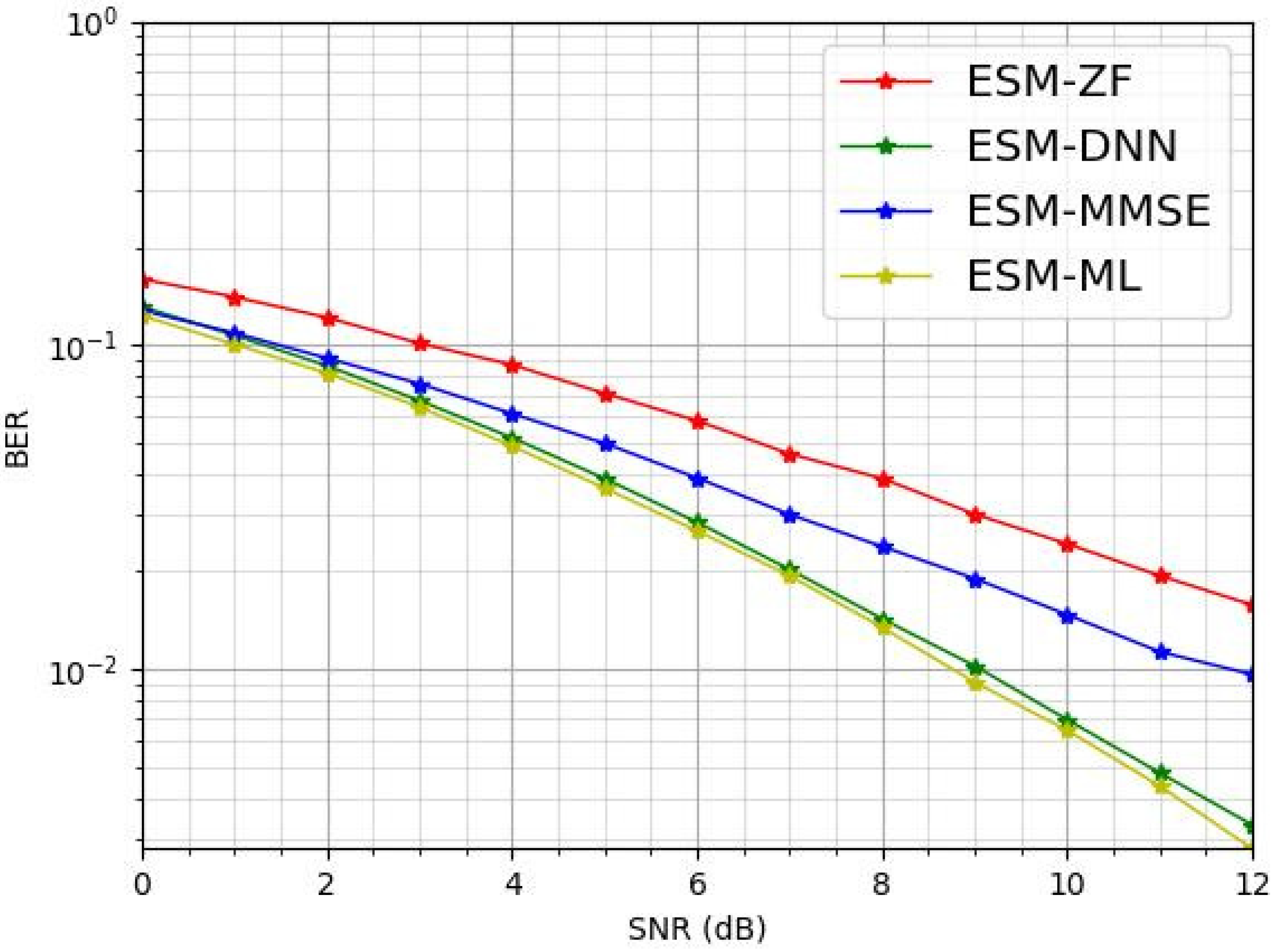
Figure 3 compares the BER performance of the proposed ESM-DNN-based detection method with other traditional detection methods, namely ML, ZF and MMSE, in a $2\times 2$ ESM communication system with QPSK modulation. As shown in Figure 3, it is clear that the ESM-ML detection approach excels in terms of BER performance. The proposed ESM-DNN detection method closely matches the BER performance of the ESM-ML method and outperforms the ESM-ZF and ESM-MMSE detection techniques.

Figure 3. The BER comparison for various detectors under $N_t$ = 2 and $N_r$ = 2.

In Figure 4, it is shown that the proposed ESM-DNN method also performs better under the $2\times 4$ ESM system configuration with QPSK modulation. Figure 4 illustrates that the ESM-ML detection method consistently achieves the optimal BER performance. Within the SNR range of 0 to 4 dB, the BER of ESM-DNN performance is as same as that of ESM-MMSE and approaches that of ESM-ML. However, as the SNR increases, the ESM-DNN method demonstrates a distinct advantage, with its BER performance starting to significantly exceed those of ESM-MMSE and ESM-ZF while remaining close to ML.

Figure 4. The BER comparison for various detectors under $N_t$ = 2 and $N_r$ = 4.

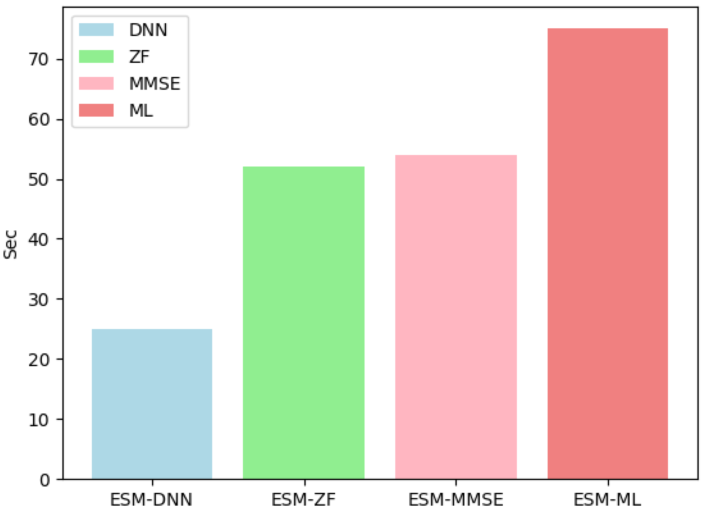
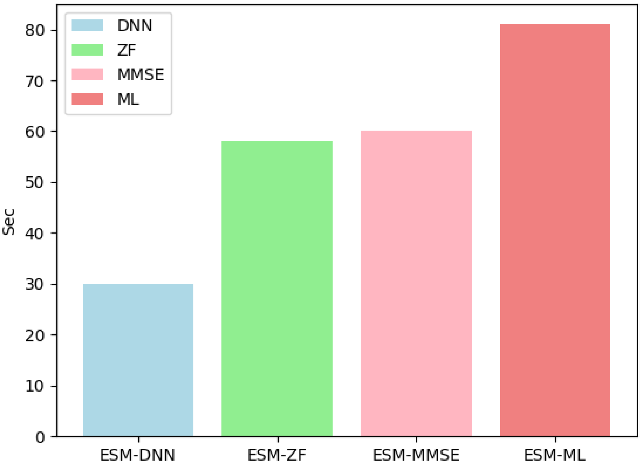
Figure 5 illustrates that ESM-DNN under the $2\times 2$ setting shows a significant advancement in runtime performance. When compared with the ML detection method, ESM-DNN reduces computational time and enhances operational efficiency. At the same time, it achieves near-optimal BER performance, thus striking a commendable balance between efficiency and accuracy. In Figure 6, when the number of antennas at the receiver increases to four, the computational time increases, but the trend of overall performance remains consistent.

Figure 5. The runtime complexity comparison for various detectors under $N_t$ = 2 and $N_r$ = 2.

Figure 6. The runtime complexity comparison for various detectors under $N_t$ = 2 and $N_r$ = 4.

The computational complexity analysis findings are summarized in Table 3. It becomes evident that the computational complexity associated with a DNN depends on the network architecture rather than the number of antennas used for transmission or reception. It is worth noting that to achieve an optimal balance between BER and computational complexity, the ESM-DNN stands out as the most suitable option.

Table 3. Computational complexity.

Detector	Real-Valued Multiply-Accumulate Operations
ESM-ML	$(2\times N_r\times N_t\times M^{N_p}+1)\times S\times C$
ESM-ZF	$N_r\times N_t\times {log}_2\left(M\right)+O\left(N_r^3\right)$
ESM-MMSE	$2\times (N_r\times N_t)+O\left(N_r^3\right)+S\times {log}_2\left(M\right)+S$
ESM-DNN	$N{N}_p((4N_r{N}_p+4N_r-1){\delta }_1+{\displaystyle \sum _{k=1}^{k=L-1}}{\delta }_{k+1}(2{\delta }_k-1))$

5. Conclusions

In this paper, a B-DNN based detection approach for the ESM system is proposed. This scheme demonstrates significant performance improvements, in both BER and computational efficiency. The numerical results confirm that the B-DNN based scheme outperforms the ZF and MMSE detection methods in terms of BER. Moreover, although the B-DNN does not surpass ML detection method in terms of BER, the proposed B-DNN method clearly excels over the ML scheme in computational demand, offering a more expeditious processing time. In the future, the advanced technology like aggregation will be considered to further improve the system performance of the proposed method.

References

- Mesleh, R.; Haas, H.; Sinanovic, S.; Ahn, C.; Yun, S. Spatial modulation. IEEE Trans. Veh. Technol. 2008, 4, 2228–2241. [Google Scholar] [CrossRef]
- Cheng, C.; Sari, H.; Sezginer, S.; Su, Y.T. Enhanced Spatial Modulation With Multiple Signal Constellations. IEEE Trans. Commun. 2015, 6, 2237–2248. [Google Scholar] [CrossRef]
- Huang, H.; Guo, S.; Gui, G.; Yang, Z.; Zhang, J.; Sari, H. Deep learning for physical-layer 5G wireless techniques: Opportunities, challenges and solutions. IEEE Wirel. Commun. 2020, 1, 214–222. [Google Scholar] [CrossRef]
- Zhu, F.; Hai, H.; Jiang, X. Efficient Antenna Selection for Adaptive Enhanced Spatial Modulation: A Deep Neural Network Approach. IEEE Commun. Lett. 2023, 5, 1352–1356. [Google Scholar] [CrossRef]
- O’Shea, T.; Hoydis, J. An introduction to deep learning for the physical layer. IEEE Trans. Cognit. Commun. Netw. 2017, 4, 563–575. [Google Scholar] [CrossRef]
- Jiang, C.; Zhang, H.; Ren, Y.; Han, Z.; Chen, C.; Han, Z. Machine learning paradigms for next-generation wireless networks. IEEE Wirel. Commun. 2017, 4, 98–105. [Google Scholar] [CrossRef]
- Dorner, S.; Cammerer, J.; Hoydis, J.; Brink, S. Deep learning based communication over the air. IEEE J. Sel. Top. Signal Process. 2018, 2, 132–143. [Google Scholar] [CrossRef]
- Aoudia, A.; Hoydis, J. End-to-end learning of communications systems without a channel model. In Proceedings of the 52nd Asilomar Conference on Signals, Systems, and Computers, Pacific Grove, CA, USA, 28–31 October 2018; pp. 298–303. [Google Scholar]
- Kim, H.; Jiang, Y.; Rana, R.; Kannan, S.; Viswanath, P. Communication algorithms via deep learning. In Proceedings of the 6th International Conference on Learning Representations, Vancouver, BC, Canada, 30 April–3 May 2018; pp. 1–17. [Google Scholar]
- Pinkus, A. Kolmogorov-Arnold neural network (KAN): A deep learning approach for function approximation. IEEE Trans. Neural Netw. Learn. Syst. 2017, 9, 2134–2145. [Google Scholar]
- Pineau, J.; Paquet, S.; Precup, D. Cognitive Computing: A Roadmap for the Future. IBM J. Res. Dev. 2016, 60, 1–10. [Google Scholar]
- Alawad, A.; Hamdi, A. A Deep Learning-Based Detector for IM-MIMO-OFDM. In Proceedings of the 2021 IEEE 94th Vehicular Technology Conference, Norman, OK, USA, 27–30 September 2021; pp. 2465–2477. [Google Scholar]
- Zhang, J.; Li, Y.; Huang, W.; Guo, H.; Yuen, C.; Guan, L. DNN-Aided Message Passing Based Block Sparse Bayesian Learning for Joint User Activity Detection and Channel Estimation. In Proceedings of the 2019 IEEE VTS Asia Pacific Wireless Communications Symposium, Singapore, 28–30 August 2019; pp. 1178–1203. [Google Scholar]
- Liao, Y.; Deng, H.; Xie, Y.; Liu, J.; Yuan, B. Low-complexity Neural Network-based MIMO Detector using Permuted Diagonal Matrix. In Proceedings of the 2020 54th Asilomar Conference on Signals, Systems, and Computers, Pacific Grove, CA, USA, 1–4 November 2020; pp. 1058–1065. [Google Scholar]
- Albinsaid, H.; Singh, K.; Biswas, S.; Li, C.P.; Alouini, M.S. Block deep neural network-based signal detector for generalized spatial modulation. IEEE Commun. Lett. 2020, 12, 2775–2779. [Google Scholar] [CrossRef]
- Shamasundar, B.; Chockalingam, A. A DNN Architecture for the Detection of Generalized Spatial Modulation Signals. IEEE Commun. Lett. 2020, 12, 2770–2773. [Google Scholar] [CrossRef]
- Zhu, J.; Deng, Y. Graph Neural Network Based Signal Detection in Quadrature Spatial Modulation System. In Proceedings of the 2023 IEEE the 23rd International Conference on Communication Technology (ICCT), NJ, CN, Wuxi, China, 20–22 October 2023; pp. 216–220. [Google Scholar]
- Shu, Y.; Peng, Y.; AL-Hazemi, F. Deep Learning Based Signal Detection for Quadrature Spatial Modulation System. China Commun. 2021, 5, 1–7. [Google Scholar]
- Mao, Q.; Hu, F.; Hao, Q. Deep learning for intelligent wireless networks: A comprehensive survey. IEEE Commun. Surv. Tutor. 2018, 4, 2595–2621. [Google Scholar] [CrossRef]
- Glorot, X.; Bordes, A.; Bengio, Y. Deep sparse rectifier neural networks. In Proceedings of the 2011 14th International Conference on Artificial Intelligence and Statistics, Fort Lauderdale, FL, USA, 11–13 April 2011; pp. 315–323. [Google Scholar]
Disclaimer/Publisher’s Note: The statements, opinions and data contained in all publications are solely those of the individual author(s) and contributor(s) and not of MDPI and/or the editor(s). MDPI and/or the editor(s) disclaim responsibility for any injury to people or property resulting from any ideas, methods, instructions or products referred to in the content. |
© 2025 by the authors. Licensee MDPI, Basel, Switzerland. This article is an open access article distributed under the terms and conditions of the Creative Commons Attribution (CC BY) license (https://creativecommons.org/licenses/by/4.0/).