4.2. Evaluation Metrics
In order to evaluate the performance of different models, some typical regression indicators are selected, such as Mean Absolute Error (MAE), Mean Square Error (MSE), and coefficient of determination ().
MAE measures the average absolute difference between the actual values and the predicted values. The advantage of MAE is its smoother treatment of errors, as it is less sensitive to extreme values, making it suitable for scenarios where the error distribution is relatively uniform. Moreover, its calculation is intuitive and easy to understand. The formula for calculating MAE is as follows:
MSE measures the average squared difference between the actual and predicted values. The advantage of MSE lies in its ability to penalize larger errors, which highlights the impact of outliers. This makes it suitable for tasks where large errors need to be particularly emphasized. The formula for calculating MSE is as follows:
is used for evaluating correlation coefficient.The advantage of
is that it measures the model’s ability to explain the variance in the data. It provides a unitless, easily interpretable relative evaluation metric, making it convenient for comparing different models. The formula for calculating
is as follows:
where
is the mean of the actual value.
4.3. Experimental Results
The model performance of all prediction models are shown in
Table 3. All evaluation indicators are the average value of the evaluation indicators obtained through five times of model fitting. It can be seen that DNM has the lowest MSE, MAE, and the highest
. The
of the DNM is 0.7405 which is higher than other models.The MSE and MAE of the DNM respectively are 12,316,995.0 and 2384.86. XGBoost mosel is the second best performing model. The
of XGBoost is 0.7286. The performance of models is shown in
Table 3.
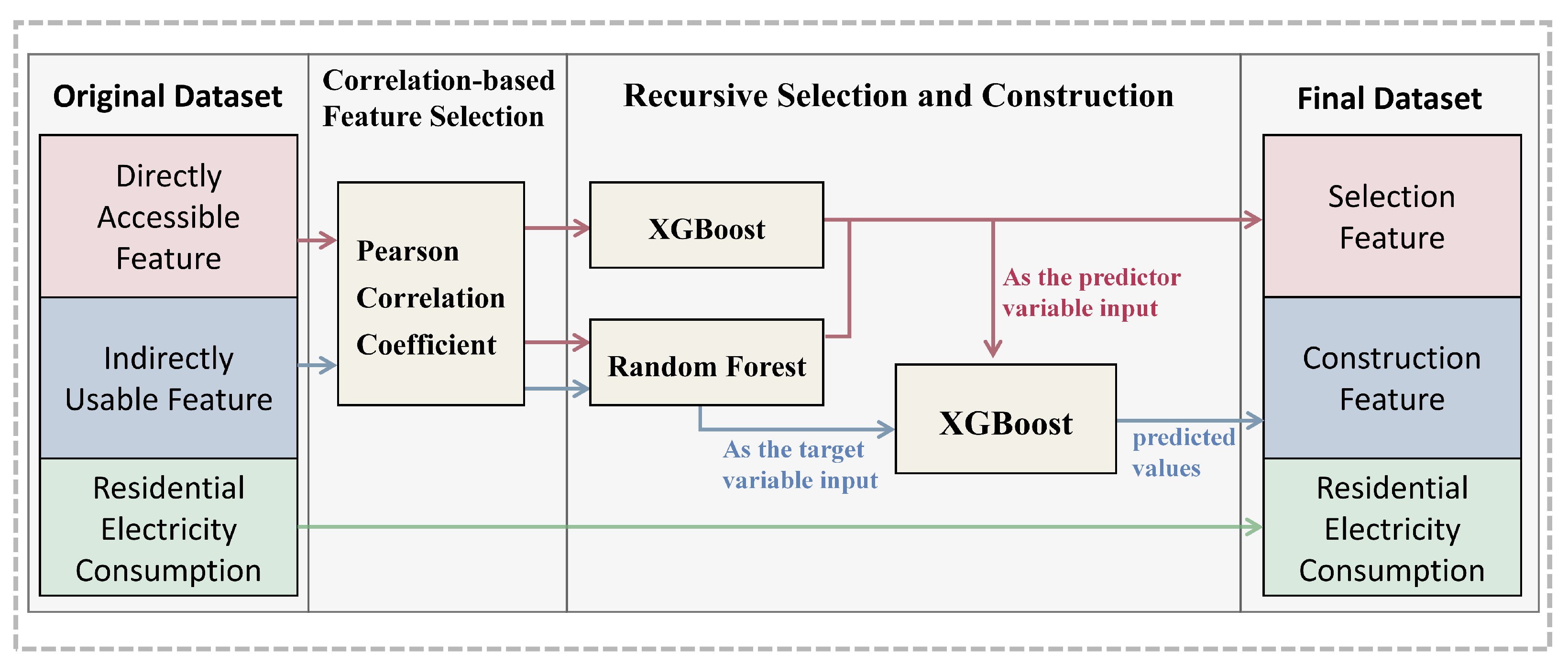
To validate the rationale behind the construction of new features based on indirectly usable ones, this study creates a new comparative dataset. This dataset contains a total of 20 features, all selected using XGBoost and Random Forest models. The new dataset is referred to as the comparison dataset, while the previous dataset is called the constructed dataset. The obtained
comparison figure for each model is shown in the
Figure 5.
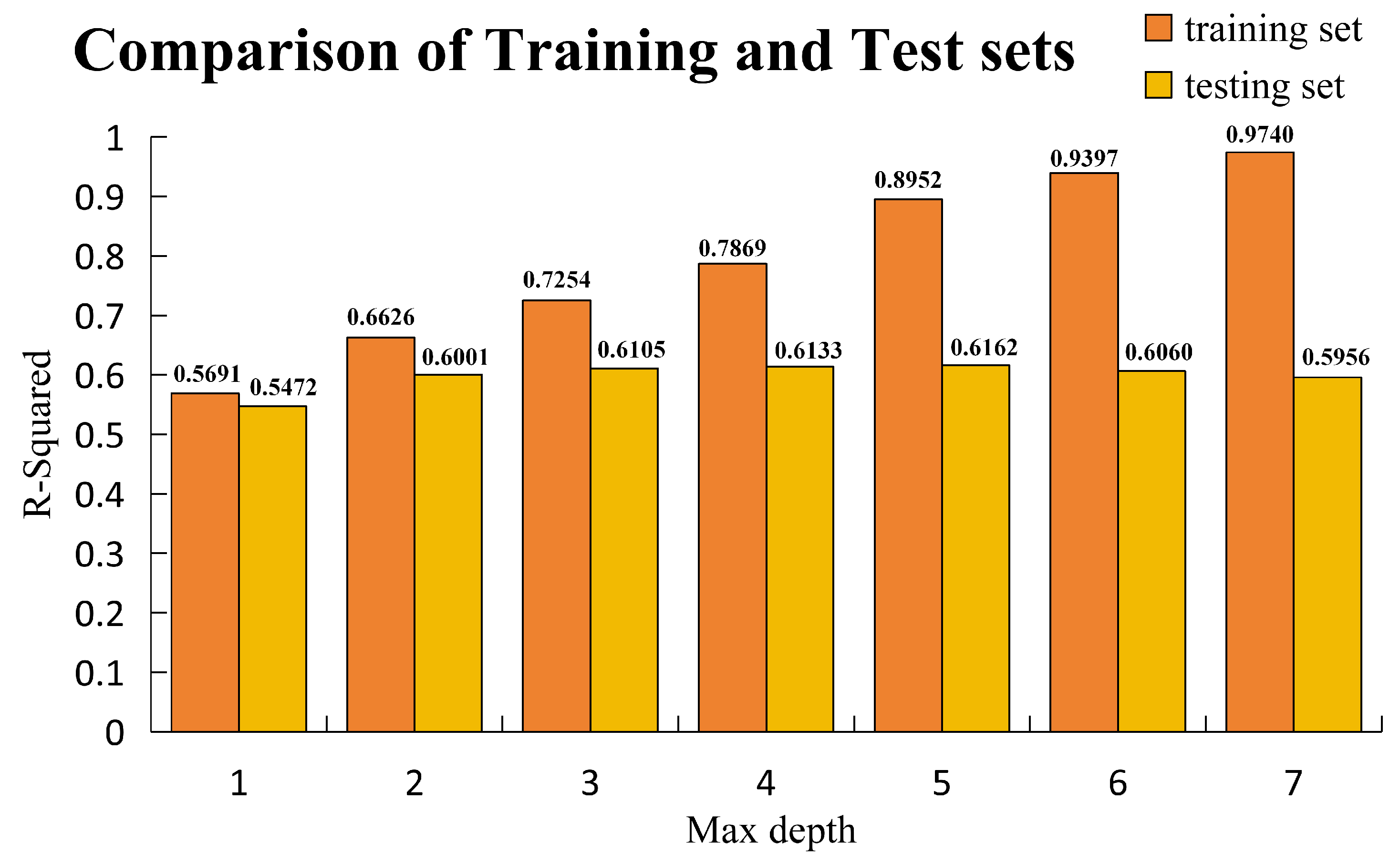
It is clear that the constructed dataset is significantly better than the comparison dataset with unconstructed variables. However, in the course of the study, it was found that the models such as XGBoost had overfitting in the comparison dataset. Therefore the XGBoost model is studied separately. In the above all the models with hyperparameters have been Bayesian tuned but still have overfitting. Because of the existence of regular terms in the XGBoost model itself, in order to further study whether the overfitting can be suppressed by the model itself, this paper chooses to manually tune the hyperparameters of the XGBoost model to suppress overfitting.Max depth is an important parameter for tuning overfitting in the XGBoost model. This paper presents the performance of the XGBoost model on training and test sets at different Max depths. The comparison is as
Figure 6.
From the
Figure 5, it is obvious that in the case of manual parameter tuning, the
of the test set does not increase but the
of the training set decreases. Therefore, the XGBoost model is unable to mitigate overfitting through its own hyperparameter adjustments. This paper chooses to make the model easier to extract information by constructing variables that cannot be obtained directly. From the
Figure 6, it is clear that the constructed variables provide significant assistance.
Also from the
Figure 6, it can be seen that the DNM model shows higher accuracy than ANN in the model and also shows very strong suppression of overfitting. On the comparison dataset, the DNM model achieves a slightly lower accuracy than the XGBoost model. However, the
of DNM model is significantly higher than other models on the constructed dataset.
Hyperparameters have a significant impact on model performance. A well-tuned model can often achieve an
score at least 0.05 higher than a model without hyperparameter tuning. However, hyperparameter tuning can be time-consuming and labor-intensive. The DNM model, with fewer hyperparameters compared to other models, significantly reduces the time required for hyperparameter optimization. At the same time, the accuracy of the DNM model is on par with or even better than other models. The runtime of each model is shown in
Table 4. The Python version is 3.9.7, with a system configuration of an Intel i9-14900HX CPU and an RTX4060 GPU. Although DNM takes more time, its performance is superior to that of other algorithms.
To validate the effectiveness of Adamax, a comparison is made with different optimization algorithms. In this paper, Adam and SGD are chosen for comparative training of the DNM model. To ensure a consistent experimental environment, the parameters of DNM are set as follows: the number of layers in the dendrite layer M = 33, and the number of iterations is set to 500. Since different optimization algorithms have varying convergence efficiencies, the learning rates are adjusted accordingly. The learning rates for Adam is set to 0.005, the learning rates for Adamax and Adagrad are set to 0.01, and the learning rate for SGD is set to 1. The results are shown in
Table 5. In comparison, Adamax and Adam perform the best, with the same accuracy, while other algorithms suffer from slower convergence or are more prone to getting stuck in local optima. Adamax converges slightly faster than Adam in practical experiments, so the algorithm chosen in this paper is Adamax.
4.4. Model Interpretation and Optimization
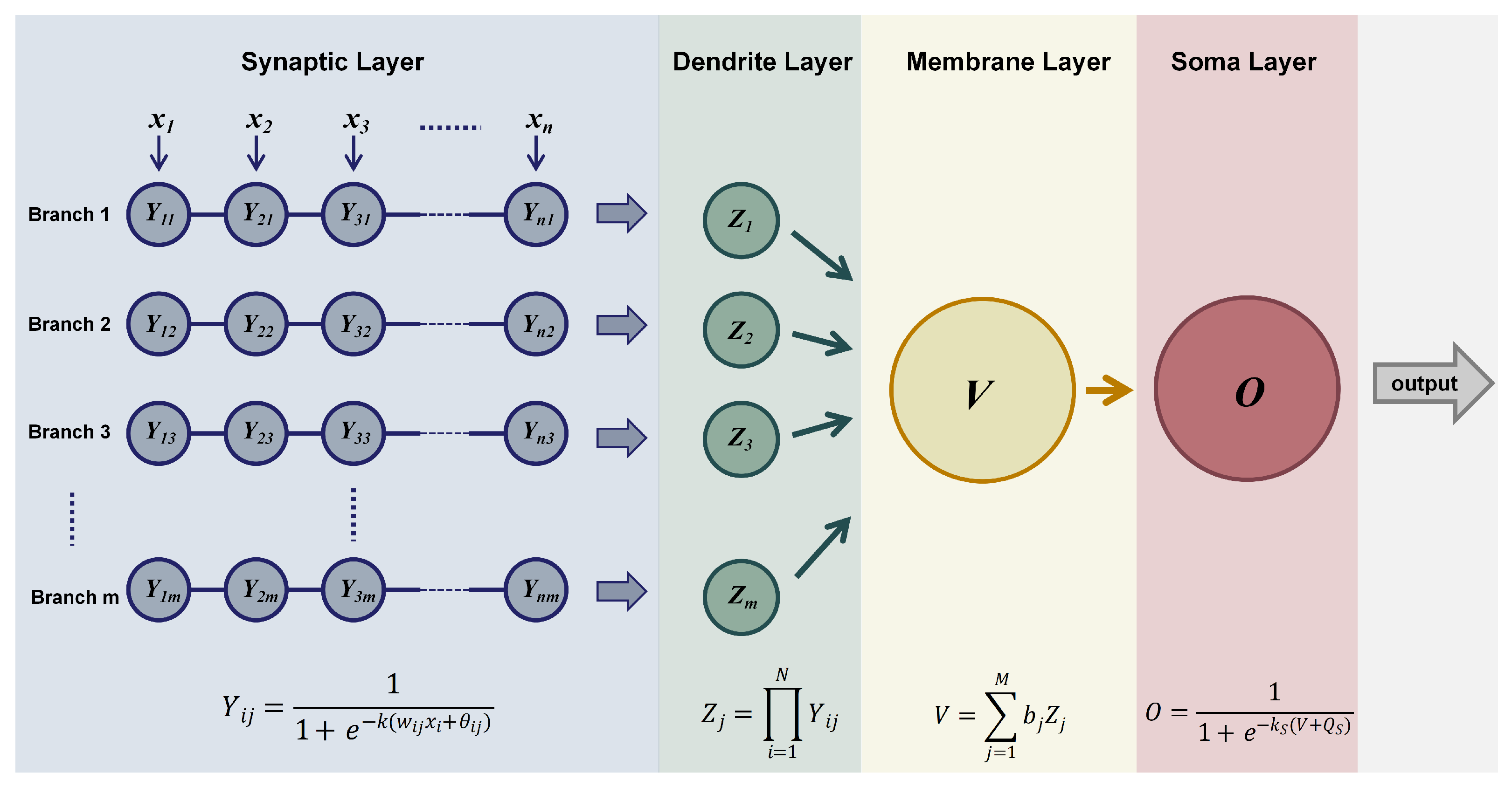
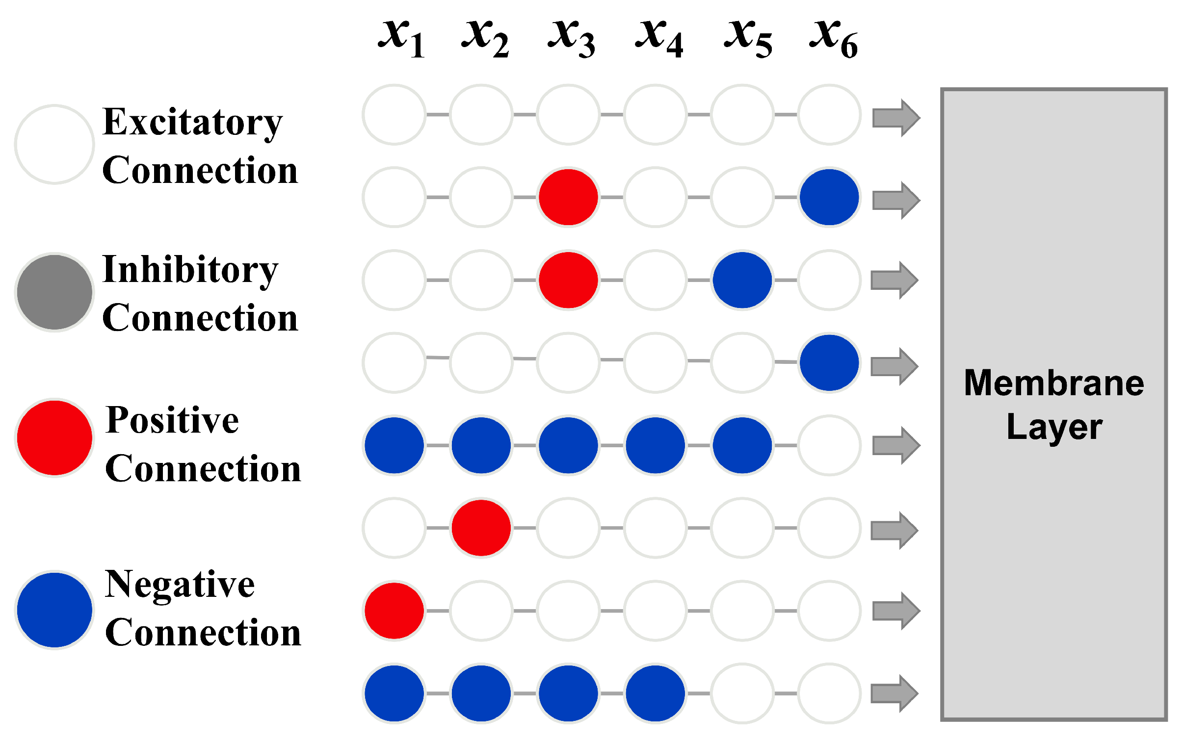
The methods of machine learning are generally black-box models, lacking strong interpretability. However, the DNM, due to its unique structure, has stronger interpretability compared to other models. This paper uses the interpretable structure of the DNM to explain the model. The greatest interpretability of the DNM is reflected in the connectivity of neurons within its dendritic layer. The image of the dendritic layer can be found in
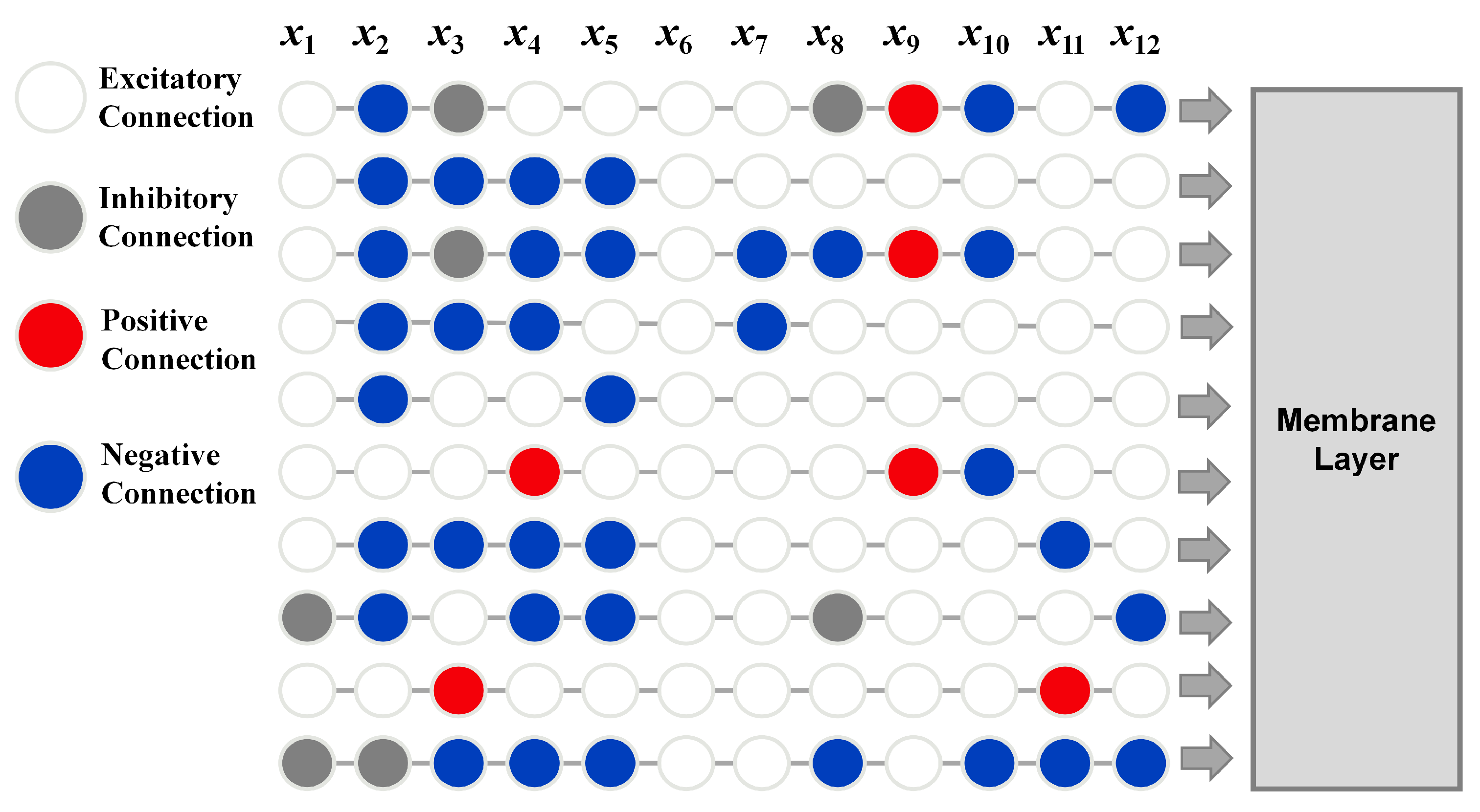
Figure 1, and different connectivity patterns in the image can be found in
Figure 2. The number of neurons for different features in the DNM is summarized in
Table 6. The feature names, labels, feature explanations, and feature value ranges can be found in the
Table 1. In this section, features are uniformly represented by feature labels.
Among the four types of connections in the dendritic layer, positive connection and negative connection represent positive and negative correlations. These two types of connections contribute the most in the dendritic layer. The output value obtained after passing a feature value through an excitatory connection is usually close to 1. However, due to the multiplicative nature of neuron connectivity, features passing through an excitatory connection not only lose their own data information but also fail to impact that branch. Thus, the larger the proportion of excitatory connections in all connection patterns for a feature, the less important the feature is. Inhibitory connections are generally considered to have a pruning effect in DNM. So, inhibitory connections also have a certain contribution to the model. In a branch, the more inhibitory connections present, the smaller the output value of that branch, making the branch more sensitive and resulting in a more accurate final prediction.
Among the four types of dendritic connections, excitatory connections have a low contribution to the model because their output remains close to 1, regardless of input size. This minimal variation has little impact on cumulative calculations, resulting in a low overall contribution to the model.
Table 6 shows that Feature 6 consists entirely of excitatory connections. Therefore, it can be considered that the contribution of this feature in the model is minimal. To verify the accuracy of the model interpretation, Feature 6 is removed, and the DNM model is fitted again using the remaining features. The resulting
value is 0.739 without any hyperparameter tuning, while the
with this variable and hyperparameter tuning is 0.7405, resulting in a difference of 0.0045. This indicates that Feature 6 contributes minimally to the model.
Among all the features, both the Random Forest and XGBoost models screened to obtain less feature contribution, which may be due to the difference in the essential structure of the tree models and the neural network models. Therefore, the information in the original data is difficult to extract.
In this paper, a stepwise screening method is employed to re-evaluate the screened features using the DNM model interpretation. The feature importance formula for the DNM model is defined as follows:
where
represents the feaure importance score of DNM model,
is the number of Positive connections,
is the number of Negative connections,
is the number of Inhibitory connections. And Excitatory connection has low contribution to the model, so its weight coefficient is 0 and does not appear in this formula. The feature importance scores of the features are shown in the
Table 7.
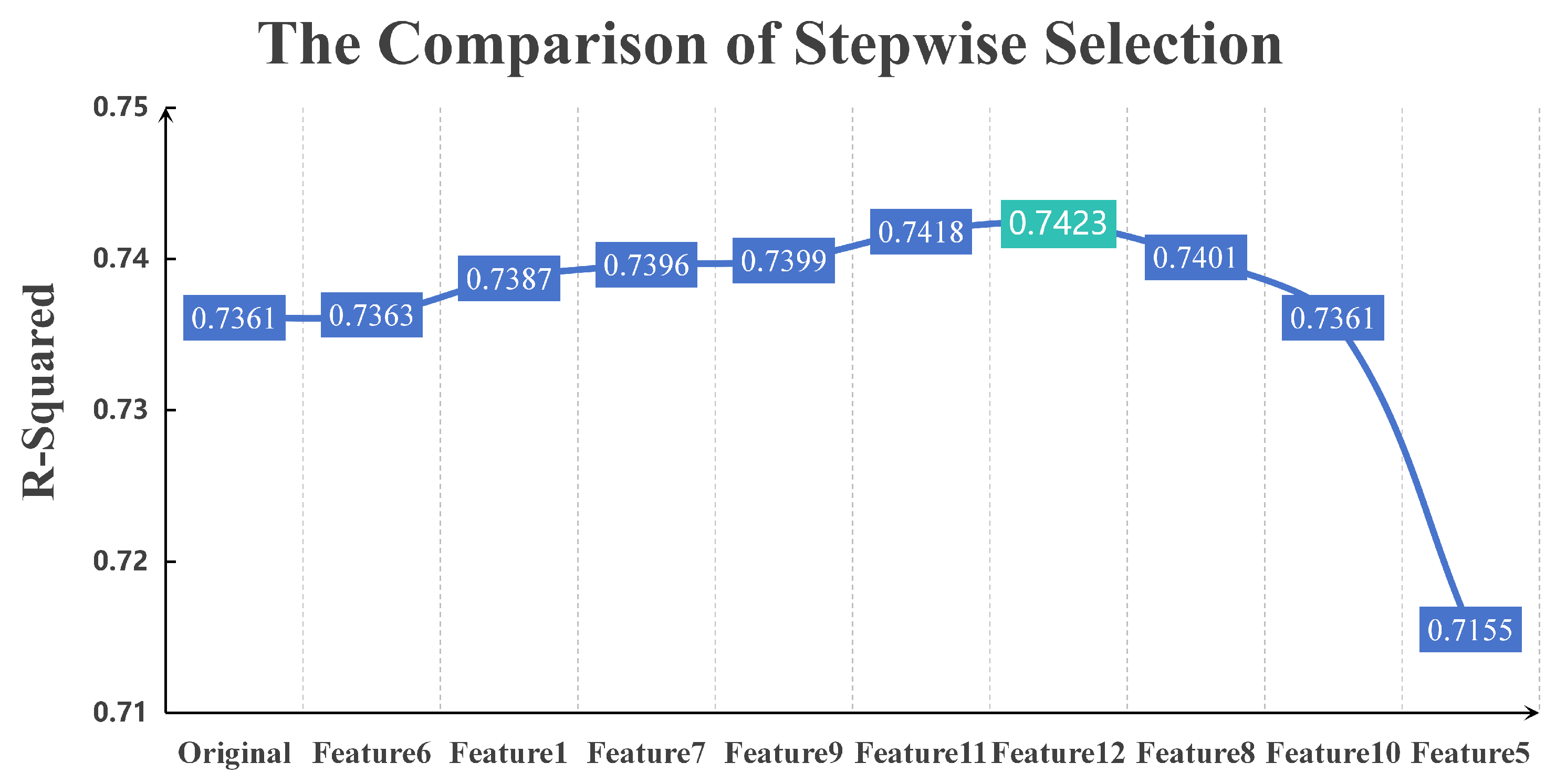
After ranking the feature importance of the DNM model, the feature with the lowest importance is removed. Then the model is fitted again, and the above steps are repeated. The sequentially removed features are Feature 6, Feature 1, Feature 7, Feature 9, Feature 11, Feature 12, Feature 8, Feature 10, and Feature 5. The
comparison plots are shown in
Figure 7, where the x-axis labels indicate the feature removed in each iteration of training. For example, at Feature 9, only eight features remain in the dataset used by the DNM model. The dataset is obtained by removing Feature 6, Feature 1, Feature 7, and Feature 9 from the constructed dataset.
From the
Figure 7, it can be clearly seen that there is a gradual increase in the model
before deleting Feaure 8 from the dataset. When features 6, 1, 7, 9, and 11 are removed, the
value gradually increases. Although the increase in
after removing each feature is small, each removal contributes positively. And the total increase is around 0.06. While after deleting Feautre 8, the performance of DNM model produces a significant decrease, and its due to the fact that the model importance of Feautre 8 is significantly higher than that of the previous variables, and there will be a significant loss of information when deleting this variable. Therefore the final feature list obtained after filtering through the DNM model feature importance is shown in
Table 8, which contains a total of six variables.
Using the above features to train the DNM model again. Also, the number of dendritic layers was reduced from 10 to 8 due to the reduction of features. The DNM dendritic architecture is obtained as follows in
Figure 8.
As can be seen from the
Figure 8, there are no features that are all excitatory connections, and there are also no inhibitory connections that represent pruning. At this point, the DNM model is optimal in terms of performance.
The DNM model’s unique construction offers interpretability which sets it apart from other neural networks. This interpretability allows for the effective elimination of unwanted features and facilitates structural tuning. As a result, the DNM model is more adaptable compared to general neural networks.
4.5. Sensitivity Analysis
To evaluate the robustness of the model, this section conducts a sensitivity analysis on the final model. In real-world residential electricity consumption forecasting, many variables are prone to errors. For example, variables such as house area and swimming pool usage time are typically provided by homeowners rather than being measured accurately, and thus may contain certain deviations. Additionally, some errors may also exist during data filtering and construction processes. Therefore, it is necessary to perform a sensitivity analysis on the DNM model.
In this study, we introduced perturbations to the final input dataset of the model to evaluate its sensitivity. Specifically, three random variables were selected from the dataset in each iteration, and perturbations with a magnitude of 0.05 (a commonly used perturbation level) were added. This process was repeated 10 times under the perturbation condition, and the model evaluations were recorded. The detailed results are presented in
Table 9.
The mean value of
in the
Table 9 is 0.6903, which differs by approximately 0.05 from the model’s performance of 0.7423 without any perturbation. This result indicates that the DNM model’s prediction
variation under noise is within an acceptable range. The model demonstrates good stability and is capable of handling the residential electricity prediction task under data perturbation.
4.6. Practical Significance
The data in this paper comes from the 2020 Residential Energy Consumption Survey, which primarily targets U.S. households. From the final model predictions, it can be seen that Features 2, 3, 4, and 5 are all components of the total electricity consumption. Feature 2 represents electricity usage excluding space heating, space cooling, and refrigerators, and it is undoubtedly closely related to the total electricity consumption. Features 3 and 4 represent the electricity consumption for space cooling and heating, which play a significant role in the total electricity consumption. This indicates that space cooling and heating are major sources of household electricity consumption. Feature 5 corresponds to the electricity consumption for water heating. Given the significant time spent on water usage in daily life, the electricity consumption for water heating contributes notably to the total electricity consumption prediction. The above features are the ones that need to be constructed. There are only two features that do not require construction: the house’s square footage and the months during which the pool was used last year. It is evident that house size is positively correlated with electricity consumption—larger houses tend to consume more electricity. As for the pool’s electricity usage, it is clearly higher than that of any other appliance, even the entire house’s consumption. Therefore, if electricity saving is desired, paying attention to the consumption of space cooling or heating, reducing the frequency of water heating, and limiting the use of the pool can be quite helpful.


