Article

A Dendritic Neural Network-Based Model for Residential Electricity Consumption Prediction

1
School of Management Science and Engineering, Nanjing Univerity of Information Science and Technology, Nanjing 210044, China
2
College of Science, Nanjing Forestry University, Nanjing 210037, China
3
Faculty of Engineering, University of Toyama, Toyama-shi 930-8555, Japan
*
Author to whom correspondence should be addressed.
Mathematics 2025, 13(4), 575; https://doi.org/10.3390/math13040575
Submission received: 27 December 2024 / Revised: 28 January 2025 / Accepted: 8 February 2025 / Published: 9 February 2025
(This article belongs to the Special Issue Biologically Plausible Deep Learning)

Abstract

:
Residential electricity consumption represents a large percentage of overall energy use. Therefore, accurately predicting residential electricity consumption and understanding the factors that influence it can provide effective strategies for reducing energy demand. In this study, a dendritic neural network-based model (DNM), combined with the AdaMax optimization algorithm, is used to predict residential electricity consumption. The case study uses the U.S. residential electricity consumption dataset.This paper constructs a feature selection framework for the dataset, reducing the high-dimensional data to 12 features. The DNM model is then used for fitting and compared with five commonly used prediction models. The R 2 of DNM is 0.7405, the highest among the six models, followed by the XGBoost model with an R 2 of 0.7286. Subsequently, the paper leverages the interpretability of DNM to further filter the data, obtaining a dataset with 6 features, and the R 2 on this dataset is further improved to 0.7423, resulting in an increase of 0.0018.

1. Introduction

Energy consumption, a crucial factor in humanity’s socioeconomic and political development, has become a key metric of civilization’s progress [1]. The amount of energy consumption is directly linked to the well-being of humans and the prosperity of the world. However, a 48% increase in the total world consumption of marketed energy is expected to occur from 2012 to 2040 according to statistics. The unprecedented level of energy consumption will have a huge environmental impact. Such a dramatic release will lead to global warming, which may put humanity in an irretrievable predicament. Therefore, it is essential for people to consider how to reduce energy consumption to mitigate its negative impacts. The building sector is responsible for around 32% of global energy consumption and nearly 40% of the total direct and indirect CO2 emission [2,3,4].
Among all types of energy usage in residential buildings, electricity has a substantial increase [5], which is expected to exceed natural gas by 2025. Therefore, residential electricity consumption analysis is a non-negligible part of the energy conservation strategy. Residential building is the basic unit, and thus the reduction of the consumption would reduce the whole society’s consumption [6,7]. It is very important to predict the residential electricity consumption and develop the strategy to reduce it. And residential electricity consumption can be affected by several factors, including building characteristic [8], occupant characteristics [7,9] and occupant behaviour [10,11]. Mainly three research methods for residential electricity consumption are simulation [10], statistical analysis [8] and machine learning [12,13,14].
However, compared to commercial buildings, few attention has been paid to residential electricity consumption prediction [15,16]. Most of the previous studies were based on statistical analysis [8,17,18,19]. Although they comprehensively explored the impact of building characteristics, occupant characteristics and occupant behaviour on building energy consumption, the possible complex relationships among building characteristics, occupant characteristics and occupant behaviour had not been well handled. Previous studies indicated that these factors may have direct or indirect impacts on building energy consumption [19,20,21]. Meanwhile, there may be non-linear relationships among these factors [22,23]. Therefore, the ability to predict residential electricity consumption with the consideration of complex relationships among factors is required to ensure the prediction accuracy. Moreover, residential electricity consumption is influenced by various features, but the relationships between these features and electricity consumption are complex and nonlinear. Traditional models, such as multiple linear regression model [8], Support Vector Machine (SVM) [24] and decision trees [25], struggle to effectively capture these nonlinear patterns. Additionally, there is significant multicollinearity among the features, which further limits the performance of traditional models in handling such complex characteristics. Therefore, neural network becomes the first choice model to predict residential electricity [26].
Dendritic Learning (DL) significantly aids in addressing issues related to spiking neural networks. Derived from Dendritic Learning, a dendritic neural network-based model (DNM) simulates the multi-layered structure of neurons and utilizes specialized activation functions to achieve logic gate transformations [27]. Furthermore, due to its neuron-simulating structure, DNM exhibits stronger nonlinear processing capabilities compared to other models like ANN. And, this paper develops DNM to make accurate forecasts on the residential electricity consumption. Building characteristics, occupant characteristics and occupant behaviours are considered as the influencing factors of electricity consumption in the model.
While the DNM possesses strong nonlinear processing capabilities, it also inherently faces the challenge of difficult parameter updates. When handling high-dimensional datasets, it is more prone to issues such as gradient explosion and gradient vanishing compared to other models. Therefore, in addressing the problem of residential electricity prediction, which involves high-dimensional datasets, this paper opts to establish a feature selection and reconstruction framework. This approach reduces the dimensionality of the dataset, transforming it into a form that can be processed by the DNM, thereby making it more suitable for handling high-dimensional data. So, this study mainly has three advantages.
  • This paper establishes a feature selection framework for residential electricity consumption, which restructures the relevant features to facilitate more effective information extraction by the model.
  • Compared to traditional neural network models, the proposed DNM model achieves superior nonlinear fitting capabilities through the activation functions of its dendritic layers and diverse connection patterns.
  • DNM model incorporates partial interpretability, allowing it to perform self-updating, self-selection, pruning, and parameter tuning autonomously—capabilities that are challenging for other models to achieve. This significantly simplifies and streamlines the model optimization process, saving both time and effort.
The remainder of this paper is structured as follows: In Section 3, the research methods are described in detail. In Section 4, the performance of the developed DNM is compared with some commonly accepted models by some typical indicators.The DNM model has a simpler structure and better accuracy compared to other models. In addition, the interpretability of the DNM model was used to further optimize the DNM, resulting in a slight improvement in prediction performance. The conclusions are presented in Section 5.

2. Architecture and Training of DNM Model

2.1. Dendritic Neural Network-Based Model

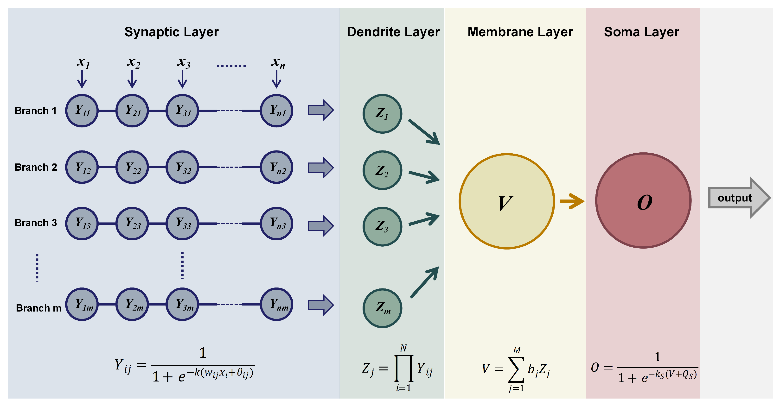
In this section, we will introduce Dendritic neural network-based model (DNM) in detail, including four layers, namely synaptic layer, dendrite layer, membrane layer and soma layer [28]. And the architecture of DNM is shown in Figure 1.
Symaptic layer is the first layer of the DNM. And this layer is mainly used to receive input features. This layer achieves multiple feature recognition and information extraction by inputting features across multiple synapses. Additionally, the use of nonlinear functions enables the extraction of nonlinear information that other models may fail to identify. The processing of the input signal by the synaptic layer can be expressed by the following Equation (1):
Y i j = 1 1 + e k w i j x i θ i j
where Y i j represents the values of ith synapse inputted to the jth dendritic branch, x i represents the ith input signal, k is a positive constant parameter, w i j represents weighting factor, and θ i j refers to threshold value. Both w i j and θ i j are determined by algorithmic learning.
Dendrite layer aggregates input signals from synapses distributed on branches [29]. This layer enhances the model’s nonlinear fitting capability by utilizing a multiplicative approach. Compared to the additive operations commonly used in traditional neural networks, multiplication better captures the correlations between features. However, this approach also increases the difficulty of model updates. To address this negative impact, the subsequent sections will introduce specific connection strategies in the dendrite layer that enable self-pruning. These strategies help improve model performance while mitigating the challenges introduced by multiplication. All values of synapses on each dendrite branch form a non-linear relationship at the dendrite layer, which can be described as follows:
Z j = i = 1 N Y i j .
where Z j indicates the output values of jth dendritic branch and N refers to the number of synapses on a branch.
The membrane layer is designed to aggregate the signals collected by the dendritic branches. It primarily simulates the processing of signals collected by multiple dendritic branches within a neuron. Therefore, this layer performs a weighted summation of the signals from the dendritic branches. This process can be expressed as follows:
V = j = 1 M b j Z j .
where V denotes the output value of membrane layer, b j is a parameter to be learned and M refers to the number of dendrite branches.
Soma layer receives dendritic signals through membrane layer and the potential changes. And the cell body will generate action, when the potential exceeds the defined threshold. The same functions as those used in the synaptic layer are applied here to further enhance the model’s performance. This process can be expressed as the follows:
O = 1 1 + e k s ( V Q s ) .
where O represents the output of soma layer, k s refers to a positive constant parameter, and Q s represents a defined threshold [30].
The DNM model structure is inspired by simulating the neurons of the human brain. The Synaptic layer and Dendrite layer simulate the synapses in the brain that receive signals. Through these two layers, information from the data can be recognized and extracted. The Membrane layer and Soma layer are responsible for processing the received signals and ultimately outputting the processed information. Compared to traditional neural networks, DNM utilizes special activation functions and multiplication rules in the Synaptic and Dendrite layers, enabling DNM to perform operations such as AND-OR gates and self-pruning. Compared to artificial neural networks, DNM has higher complexity and performs better in recognizing nonlinear relationships.
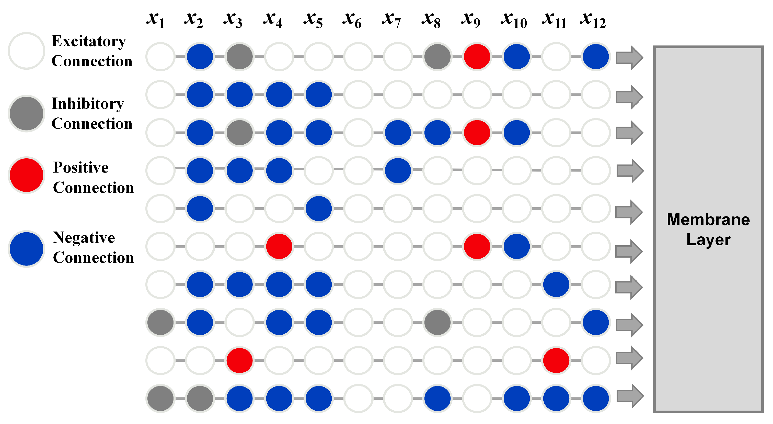
According to different combinations of w i j and θ i j , synapses can be categorized into six combinations. Four of these types are combined into two connection cases. So there are four types of connection cases, namely excitatory connection, inhibitory connection, positive connection and negative connection, as shown in Figure 2. When the value of w i j is greater than 0, x and y are positively correlated. Conversely, when w i j is less than 0, x and y are negatively correlated. Regarding the parameter θ i j , when θ i j is greater than both 0 and w i j , the synapse exhibits a form as a inhibitory connection. When θ i j is less than both 0 and w i j , the synapse is a excitatory connection. When θ i j is between 0 and w i j , the synapse displays an active mode. Four kinds of connection cases are listed as follow:
  • Positive connection ( 0 < θ i j < w i j ). In this case, the output value exhibits a positive correlation with the input data, meaning that any change in the input will result in a significant change in the output. As a result, this type of connection is referred to as a positive connection.
  • Negative connection ( w i j < θ i j < 0 ). In this case, the output value exhibits a negative correlation with the input data, meaning that any change in the input will result in a significant change in the output. As a result, this type of connection is referred to as a negative connection.
  • Excitatory connection ( θ i j < w i j < 0 or θ i j < 0 < w i j ). In this case, regardless of how the input signal x i varies, the output from the synaptic layer will approach 1. In the multiplication model, values approaching 1 have minimal impact on the model. Therefore, this type of connection indicates that the corresponding feature has no significant influence on this particular branch.
  • Inhibitory connection ( w i j < 0 < θ i j or 0 < w i j < θ i j ). In this case, regardless of how the input signal x i varies, the output from the synaptic layer will approach 0. In the multiplication model, if any value approaches 0, the output value will also approach 0. This characteristic endows this type of connection with a pruning function within the model. For the increased difficulty in model updates introduced by the multiplication approach, the presence of inhibitory connections enables the model to perform self-pruning. By doing so, the model can appropriately reduce its complexity during updates, effectively counteracting the negative effects of the multiplication mechanism while preserving its benefits.
Figure 2. Four types of connection cases.
Mathematics 13 00575 g002
Among the four types of connections, positive and negative connections contribute the most to the model. Inhibitory connections function similarly to pruning; an excess of this connection suggests that the model has too many dendritic layers, acting as an internal mechanism to prevent overfitting. In contrast, excitatory connections output values close to 1, which have minimal impact on the final model. Therefore, in the context of the model, this connection type indicates that the corresponding variable contributes little to that branch.

2.2. Learning Algorithm

AdaMax is used to train the DNM in this research. It is a variant of the popular Adam optimizer and is designed to provide a simpler range for the upper limit of the learning rate than Adam. The Adam optimizer uses a moving average of past gradients and past squared gradients to adaptively update the learning rate for each parameter during training. The AdaMax optimizer is a variant of the Adam optimizer. Unlike Adam, AdaMax replaces the L2 norm used in the second moment estimation of Adam with a max norm. However, its first moment estimation is similar to that of Adam.
The output value V of DNM is compared with the real value T. The error E between V and T can be expressed as follows:
E = 1 2 ( T V ) 2 .
The parameters w, θ and b in DNM model are continuously modified by AdaMax. The partial derivative of E with respect to w, θ and b can be expressed as follows:
δ ω i j = E ω i j = E V × V Z j × Z j Y i j × Y i j ω i j = ( V T ) × b j × L = 1 L i N Y L j × k x i e k ( x i ω i j θ i j ) ( 1 + e k x i ω i j θ i j ) 2 , δ θ i j = E θ i j = E V × V Z j × Z j Y i j × Y i j θ i j = ( V T ) × b j × L = 1 L i N Y L j × k e k ( x i ω i j θ i j ) ( 1 + e k x i ω i j θ i j ) 2 , δ b j = E b j = E V × V b j = ( V T ) × Z j .
According to Adam, m t is defined as the exponential moving average of the partial derivative with respect to parameters, such as w and θ in the t-th iteration, and v t is defined as the exponential moving average of the squared partial derivative with respect to parameters, such as w and θ , which can be described as follows:
m t = β 1 v m ( t 1 ) + ( 1 β 1 ) g t ,
v t = β 2 v t 1 + ( 1 β 2 ) g t 2 .
However, AdaMax is used to replace the Adam in this research. Unlike the Adam, AdaMax replace the L2 norm with a max norm, which can be described as follows:
v t = β 2 v t 1 + ( 1 β 2 ) | g t | = max ( β 2 · v t 1 , | g t | ) .
The update equations for w, θ and b are the same, and the equation can be expressed as follows:
Φ t + 1 = Φ t η v t + ϵ m t .
where Φ represents w, θ or b. And η is learning rate, ϵ is a constant with the value of 0.00001.

3. Data Pre-Processing and Experiments

In this section, we will preprocess the collected data and input it into the model. The residential electricity consumption data is sourced from the 2020 Residential Energy Consumption Survey (https://www.eia.gov/consumption/residential, accessed on 26 December 2024). The data was collected from 18496 households and includes 799 features. The training set and testing set are divided in a ratio of 7:3, and the division is performed randomly.

3.1. Data Cleaning and Normalization

Before developing the model and analyzing the data, data preparation is necessary to ensure data quality. The data preparation process consists of three phases. In the first phase, any samples with missing data are deleted from the dataset. Out of 18,496 samples, 274 samples with missing values were removed.
In the second phase of data preparation, outliers in the dataset are eliminated. Outliers are typically data errors that can negatively impact model training and evaluation. In this paper, the Z-score method is chosen to handle outliers. The formula for Z-score is as follows:
Z = X μ σ
where μ is the mean and σ is standard deviation. A Z-score above 3 indicates that the data point is far above the mean, while a Z-score below −3 indicates that it is far below the mean. Data points with Z-scores outside the range of 3 , 3 are generally flagged as outliers.
In the third phase, the unreasonable data are removed or reassigned. There are some categorized features that are assigned with abnormal value such as 99 which is much larger than other normal classification values. Therefore, this paper chooses two ways to deal with these unreasonable data. When there are only a few unreasonable assignment samples in a categorized feature, these samples are deleted. When a categorical variable contains several unreasonable samples, 0 or other smaller values are used to replace them, preventing any negative impact on the model’s prediction performance. It is generally reset to −3.
Eventually 18,116 samples remained. After handling missing values and outliers, the data is standardized using Z-score normalization. The formula is as follows:
Z = X μ σ
where μ is the mean and σ is standard deviation.

3.2. Feature Selection and Construction

After processing the samples, the features need to be screened and constructed. In this dataset, there are 799 features. We treat residential electricity consumption as the dependent variable and use the remaining 798 features as independent variables. Among these 798 features, there are two types: directly accessible features and indirectly usable features.
Indirectly usable features refer to variables that are highly correlated with the dependent variable in real-world scenarios. For example, the electricity bill is directly related to electricity consumption, as it is calculated based on the amount of energy used. Therefore, using the electricity bill to predict consumption would be unreasonable. These features are classified as indirectly usable features. However, since these variables exist in past real-world data and can be collected in practical scenarios, removing them would result in a significant loss of information, which would hinder the model’s ability to fully leverage all available data.
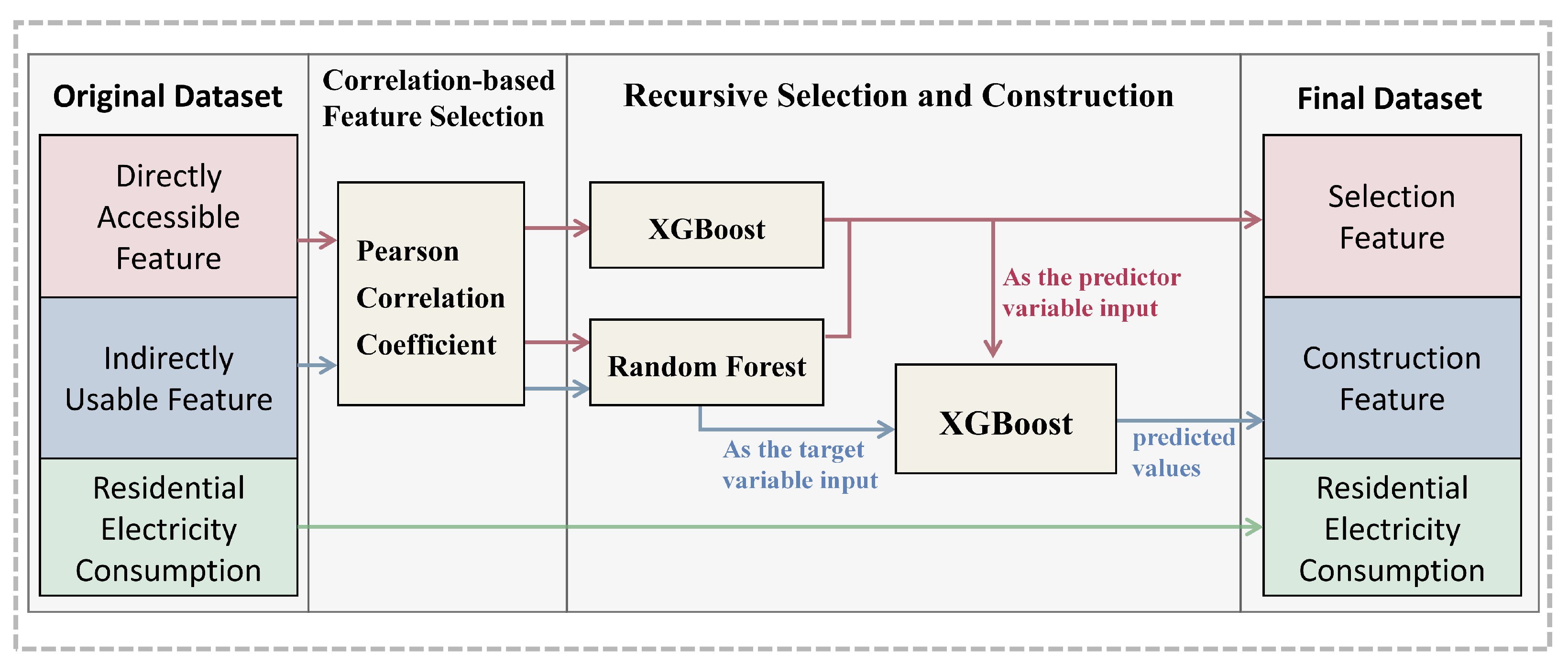
To address this, this study chooses to build a model that uses directly accessible features to predict the indirectly usable features. The predicted values of the indirectly usable features are then used as features to predict residential electricity consumption. This approach preserves the causal relationships between variables in real life while making full use of the information provided by these variables.The flowchart is shown in Figure 3.
The specific steps are as follows: First, we use the correlation coefficient-based feature selection method to remove features with high correlation. The correlation coefficient chosen is the Pearson correlation coefficient, with a threshold set at 0.9. The formula for the Pearson correlation coefficient is as follows:
r = ( X i X ¯ ) ( Y i Y ¯ ) ( X i X ¯ ) 2 ( Y i Y ¯ ) 2
where X i and Y i are the individual data points of variables X and Y, X ¯ and Y ¯ are the means of variables X and Y.
Next, for the directly accessible features, the Random Forest and XGBoost models are used for feature selection. Both the XGBoost and Random Forest models are fitted to the entire dataset, and the corresponding feature importance is output. Then, the features are ranked from high to low based on their importance, and the top five features with the highest importance are retained. Each model selects five variables, which are then used as the independent variables in the final dataset. Some overlap exists between the features selected by the two models, resulting in a final set of 7 unique features.
Then, for the indirectly usable features, the Random Forest model is used to select five features. Afterward, using the selected directly accessible features, an XGBoost model is built for each of the five indirectly usable features to make predictions. The predicted values are included as constructed variables in the final dataset, serving as independent variables.
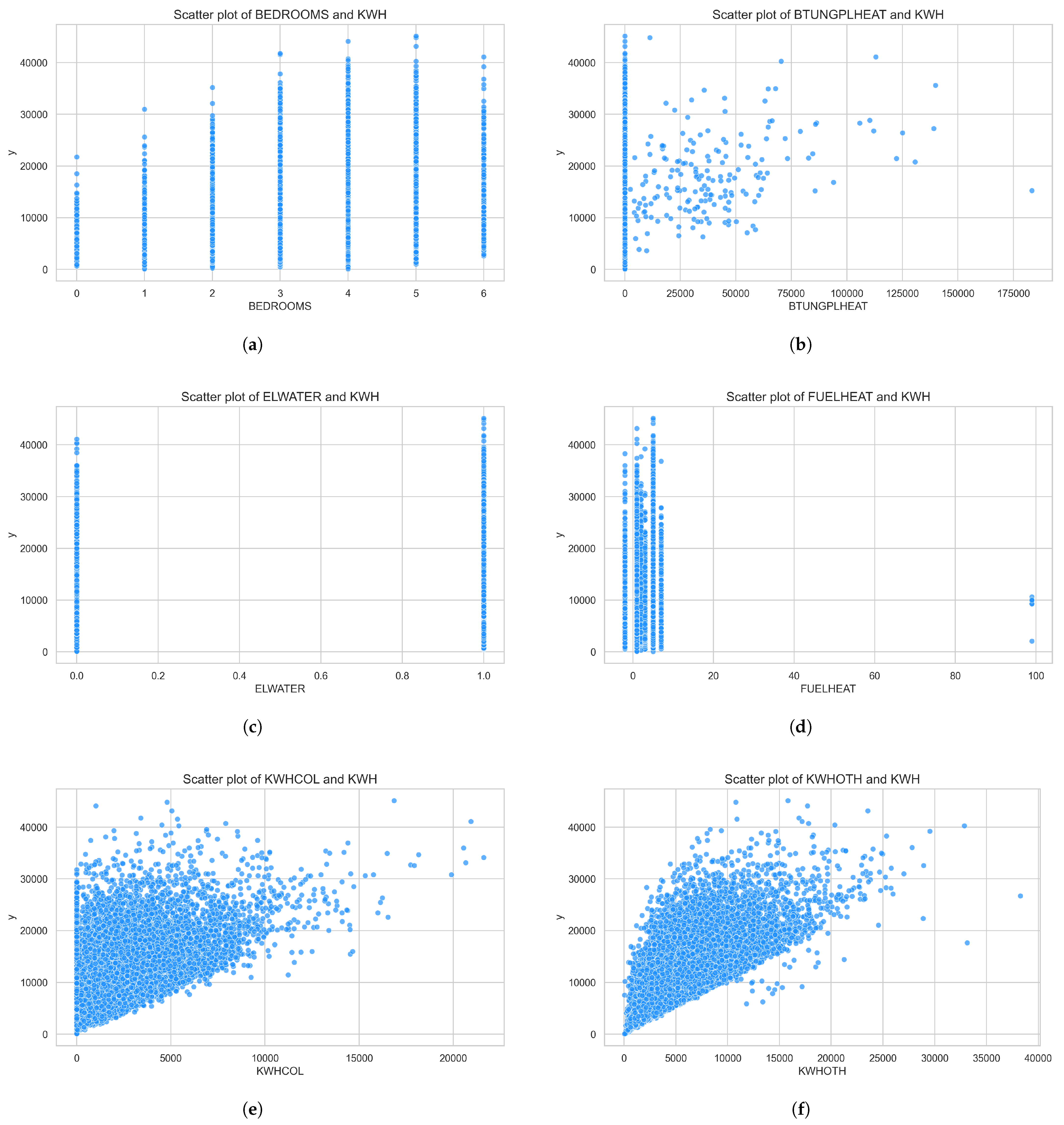
The final dataset contains 12 independent variables and 1 dependent variable, which is residential electricity consumption. The description of independent variables in final dataset is provided in Table 1. The scatter plots of the predictor variable (residential electricity consumption) and other dependent variables will be presented in Appendix A.

3.3. Execution Model

The DNM has four hyperparameters that need to be set: the number of epochs, the number of dendrite layers, the k value in Equation (1), and the initial learning rate. Increasing the number of epochs brings the model closer to the optimum solution. However, a higher number of epochs also increases the required training time. After careful consideration and multiple attempts, this paper sets the epoch count of the model to 1500.
We choose Bayesian optimization to adjust the hyperparameters of the DNM. Bayesian optimization is a black-box algorithm used to optimize objective functions. It combines Bayesian inference and optimization techniques to effectively handle complex optimization problems involving high dimensions and noise interference. The core idea of Bayesian optimization is to iteratively select sample points for evaluation in order to gradually optimize the objective function [31]. Bayesian optimization is a probabilistic global optimization model that uses Gaussian processes, a non-parametric statistical method, to describe the distribution space of the objective function. By utilizing the existing prediction information, it predicts the most optimal points in the space at each iteration, and iterates this process to approach the global optimum.
The hyperparameters required for Bayesian optimization include the k, the initial learning rate, and the number of dendritic layers. The range for k is set from 0 to 10, for the initial learning rate from 0.000001 to 0.1, and for the dendritic layers from 5 to 50. Bayesian optimization utilizes four initial points and twenty update points. The optimal results from Bayesian optimization yielded a k value of 1.4, an initial learning rate of 0.005, and 33 dendritic layers.
The optimal hyperparameters of the model, with the k value of 1.4, the initial learning rate of 0.005, and 33 dendritic layers, are set. After setting the hyperparameters, the DNM is trained, and the AdaMax algorithm is used for parameter optimization. The specific parameter updates and update methods are detailed in Section 2.2. The dendritic layer structure is shown in Figure 4.

4. Results and Discussion

4.1. Compared Models

In terms of model comparison, this paper selected six models to compare with DNM, namely SVM, XGBoost, Random Forest, LightGBM, ANN and Transformer. The models are implemented and run using Python. The SVM and Random Forest models are implemented using functions from the sklearn package, while the ANN and Transformer models are built using functions from the pytorch package. The XGBoost and LightGBM models are implemented using the xgboost and lightgbm libraries, respectively. Among the models considered, SVM is a machine learning algorithm used for both classification and regression tasks. It has been widely applied in residential electricity consumption prediction due to its excellent performance and strong mathematical foundation. XGBoost, LightGBM, and Random Forest are all tree-based models. These models have been widely used in residential electricity consumption prediction and other similar forecasting tasks, consistently demonstrating good performance. ANN is a fundamental neural network model. It is frequently used for numerical prediction tasks and enjoys widespread acceptance in the field. Since both ANN and DNM belong to the family of neural network models, ANN is included in this study as a baseline for comparison. Transformer, a model derived from the attention mechanism, is predominantly used in natural language processing. However, recent studies have also explored its application in numerical data prediction and image recognition. Therefore, this paper includes Transformer as a comparative model to evaluate its performance against other approaches. Among them, the optimal hyperparameters of the Random Forest model, LightGBM, XGBoost ANN and SVM are also obtained by using Bayesian optimization. However, due to the significantly higher complexity of the Transformer model compared to other models, and considering that there should not be a significant difference in the running time and cost of the models compared in this paper, only a simple grid search for hyperparameter tuning is performed for the Transformer model. Optimal Hyperparameters is shown in Table 2.

4.2. Evaluation Metrics

In order to evaluate the performance of different models, some typical regression indicators are selected, such as Mean Absolute Error (MAE), Mean Square Error (MSE), and coefficient of determination ( R 2 ).
MAE measures the average absolute difference between the actual values and the predicted values. The advantage of MAE is its smoother treatment of errors, as it is less sensitive to extreme values, making it suitable for scenarios where the error distribution is relatively uniform. Moreover, its calculation is intuitive and easy to understand. The formula for calculating MAE is as follows:
MAE = i = 1 n | T i V i | / n .
MSE measures the average squared difference between the actual and predicted values. The advantage of MSE lies in its ability to penalize larger errors, which highlights the impact of outliers. This makes it suitable for tasks where large errors need to be particularly emphasized. The formula for calculating MSE is as follows:
MSE = i = 1 n ( T i V i ) 2 / n .
R 2 is used for evaluating correlation coefficient.The advantage of R 2 is that it measures the model’s ability to explain the variance in the data. It provides a unitless, easily interpretable relative evaluation metric, making it convenient for comparing different models. The formula for calculating R 2 is as follows:
R 2 = 1 i = 1 n ( T i V i ) 2 i = 1 n ( T i T ¯ i ) 2
where T ¯ i is the mean of the actual value.

4.3. Experimental Results

The model performance of all prediction models are shown in Table 3. All evaluation indicators are the average value of the evaluation indicators obtained through five times of model fitting. It can be seen that DNM has the lowest MSE, MAE, and the highest R 2 . The R 2 of the DNM is 0.7405 which is higher than other models.The MSE and MAE of the DNM respectively are 12,316,995.0 and 2384.86. XGBoost mosel is the second best performing model. The R 2 of XGBoost is 0.7286. The performance of models is shown in Table 3.
To validate the rationale behind the construction of new features based on indirectly usable ones, this study creates a new comparative dataset. This dataset contains a total of 20 features, all selected using XGBoost and Random Forest models. The new dataset is referred to as the comparison dataset, while the previous dataset is called the constructed dataset. The obtained R 2 comparison figure for each model is shown in the Figure 5.
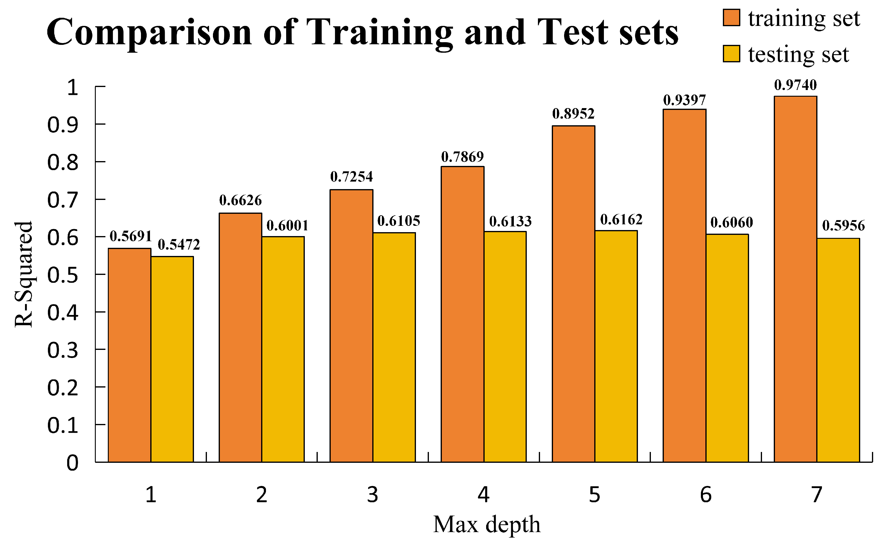
It is clear that the constructed dataset is significantly better than the comparison dataset with unconstructed variables. However, in the course of the study, it was found that the models such as XGBoost had overfitting in the comparison dataset. Therefore the XGBoost model is studied separately. In the above all the models with hyperparameters have been Bayesian tuned but still have overfitting. Because of the existence of regular terms in the XGBoost model itself, in order to further study whether the overfitting can be suppressed by the model itself, this paper chooses to manually tune the hyperparameters of the XGBoost model to suppress overfitting.Max depth is an important parameter for tuning overfitting in the XGBoost model. This paper presents the performance of the XGBoost model on training and test sets at different Max depths. The comparison is as Figure 6.
From the Figure 5, it is obvious that in the case of manual parameter tuning, the R 2 of the test set does not increase but the R 2 of the training set decreases. Therefore, the XGBoost model is unable to mitigate overfitting through its own hyperparameter adjustments. This paper chooses to make the model easier to extract information by constructing variables that cannot be obtained directly. From the Figure 6, it is clear that the constructed variables provide significant assistance.
Also from the Figure 6, it can be seen that the DNM model shows higher accuracy than ANN in the model and also shows very strong suppression of overfitting. On the comparison dataset, the DNM model achieves a slightly lower accuracy than the XGBoost model. However, the R 2 of DNM model is significantly higher than other models on the constructed dataset.
Hyperparameters have a significant impact on model performance. A well-tuned model can often achieve an R 2 score at least 0.05 higher than a model without hyperparameter tuning. However, hyperparameter tuning can be time-consuming and labor-intensive. The DNM model, with fewer hyperparameters compared to other models, significantly reduces the time required for hyperparameter optimization. At the same time, the accuracy of the DNM model is on par with or even better than other models. The runtime of each model is shown in Table 4. The Python version is 3.9.7, with a system configuration of an Intel i9-14900HX CPU and an RTX4060 GPU. Although DNM takes more time, its performance is superior to that of other algorithms.
To validate the effectiveness of Adamax, a comparison is made with different optimization algorithms. In this paper, Adam and SGD are chosen for comparative training of the DNM model. To ensure a consistent experimental environment, the parameters of DNM are set as follows: the number of layers in the dendrite layer M = 33, and the number of iterations is set to 500. Since different optimization algorithms have varying convergence efficiencies, the learning rates are adjusted accordingly. The learning rates for Adam is set to 0.005, the learning rates for Adamax and Adagrad are set to 0.01, and the learning rate for SGD is set to 1. The results are shown in Table 5. In comparison, Adamax and Adam perform the best, with the same accuracy, while other algorithms suffer from slower convergence or are more prone to getting stuck in local optima. Adamax converges slightly faster than Adam in practical experiments, so the algorithm chosen in this paper is Adamax.

4.4. Model Interpretation and Optimization

The methods of machine learning are generally black-box models, lacking strong interpretability. However, the DNM, due to its unique structure, has stronger interpretability compared to other models. This paper uses the interpretable structure of the DNM to explain the model. The greatest interpretability of the DNM is reflected in the connectivity of neurons within its dendritic layer. The image of the dendritic layer can be found in Figure 1, and different connectivity patterns in the image can be found in Figure 2. The number of neurons for different features in the DNM is summarized in Table 6. The feature names, labels, feature explanations, and feature value ranges can be found in the Table 1. In this section, features are uniformly represented by feature labels.
Among the four types of connections in the dendritic layer, positive connection and negative connection represent positive and negative correlations. These two types of connections contribute the most in the dendritic layer. The output value obtained after passing a feature value through an excitatory connection is usually close to 1. However, due to the multiplicative nature of neuron connectivity, features passing through an excitatory connection not only lose their own data information but also fail to impact that branch. Thus, the larger the proportion of excitatory connections in all connection patterns for a feature, the less important the feature is. Inhibitory connections are generally considered to have a pruning effect in DNM. So, inhibitory connections also have a certain contribution to the model. In a branch, the more inhibitory connections present, the smaller the output value of that branch, making the branch more sensitive and resulting in a more accurate final prediction.
Among the four types of dendritic connections, excitatory connections have a low contribution to the model because their output remains close to 1, regardless of input size. This minimal variation has little impact on cumulative calculations, resulting in a low overall contribution to the model. Table 6 shows that Feature 6 consists entirely of excitatory connections. Therefore, it can be considered that the contribution of this feature in the model is minimal. To verify the accuracy of the model interpretation, Feature 6 is removed, and the DNM model is fitted again using the remaining features. The resulting R 2 value is 0.739 without any hyperparameter tuning, while the R 2 with this variable and hyperparameter tuning is 0.7405, resulting in a difference of 0.0045. This indicates that Feature 6 contributes minimally to the model.
Among all the features, both the Random Forest and XGBoost models screened to obtain less feature contribution, which may be due to the difference in the essential structure of the tree models and the neural network models. Therefore, the information in the original data is difficult to extract.
In this paper, a stepwise screening method is employed to re-evaluate the screened features using the DNM model interpretation. The feature importance formula for the DNM model is defined as follows:
P score = N Pos + N Neg + 0.5 N Inhi .
where P score represents the feaure importance score of DNM model, N Pos is the number of Positive connections, N Neg is the number of Negative connections, N Inhi is the number of Inhibitory connections. And Excitatory connection has low contribution to the model, so its weight coefficient is 0 and does not appear in this formula. The feature importance scores of the features are shown in the Table 7.
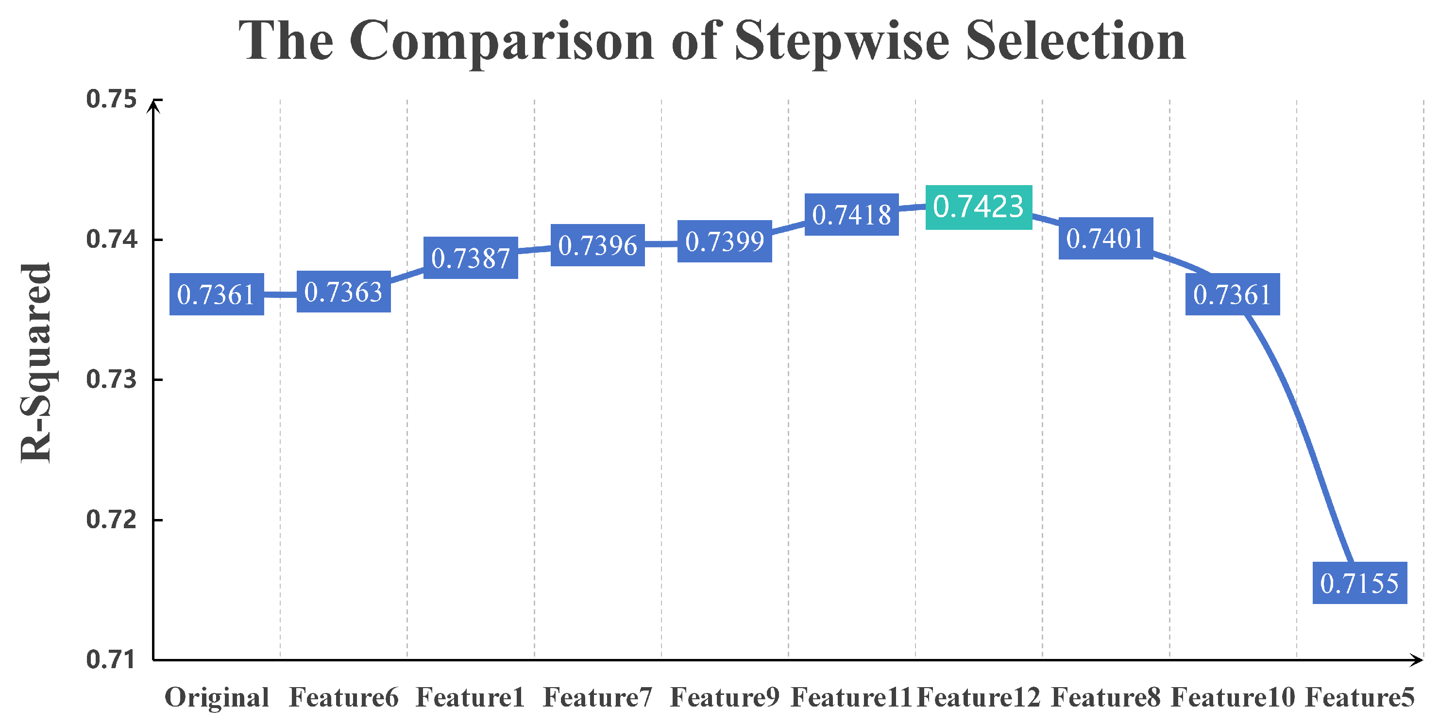
After ranking the feature importance of the DNM model, the feature with the lowest importance is removed. Then the model is fitted again, and the above steps are repeated. The sequentially removed features are Feature 6, Feature 1, Feature 7, Feature 9, Feature 11, Feature 12, Feature 8, Feature 10, and Feature 5. The R 2 comparison plots are shown in Figure 7, where the x-axis labels indicate the feature removed in each iteration of training. For example, at Feature 9, only eight features remain in the dataset used by the DNM model. The dataset is obtained by removing Feature 6, Feature 1, Feature 7, and Feature 9 from the constructed dataset.
From the Figure 7, it can be clearly seen that there is a gradual increase in the model R 2 before deleting Feaure 8 from the dataset. When features 6, 1, 7, 9, and 11 are removed, the R 2 value gradually increases. Although the increase in R 2 after removing each feature is small, each removal contributes positively. And the total increase is around 0.06. While after deleting Feautre 8, the performance of DNM model produces a significant decrease, and its due to the fact that the model importance of Feautre 8 is significantly higher than that of the previous variables, and there will be a significant loss of information when deleting this variable. Therefore the final feature list obtained after filtering through the DNM model feature importance is shown in Table 8, which contains a total of six variables.
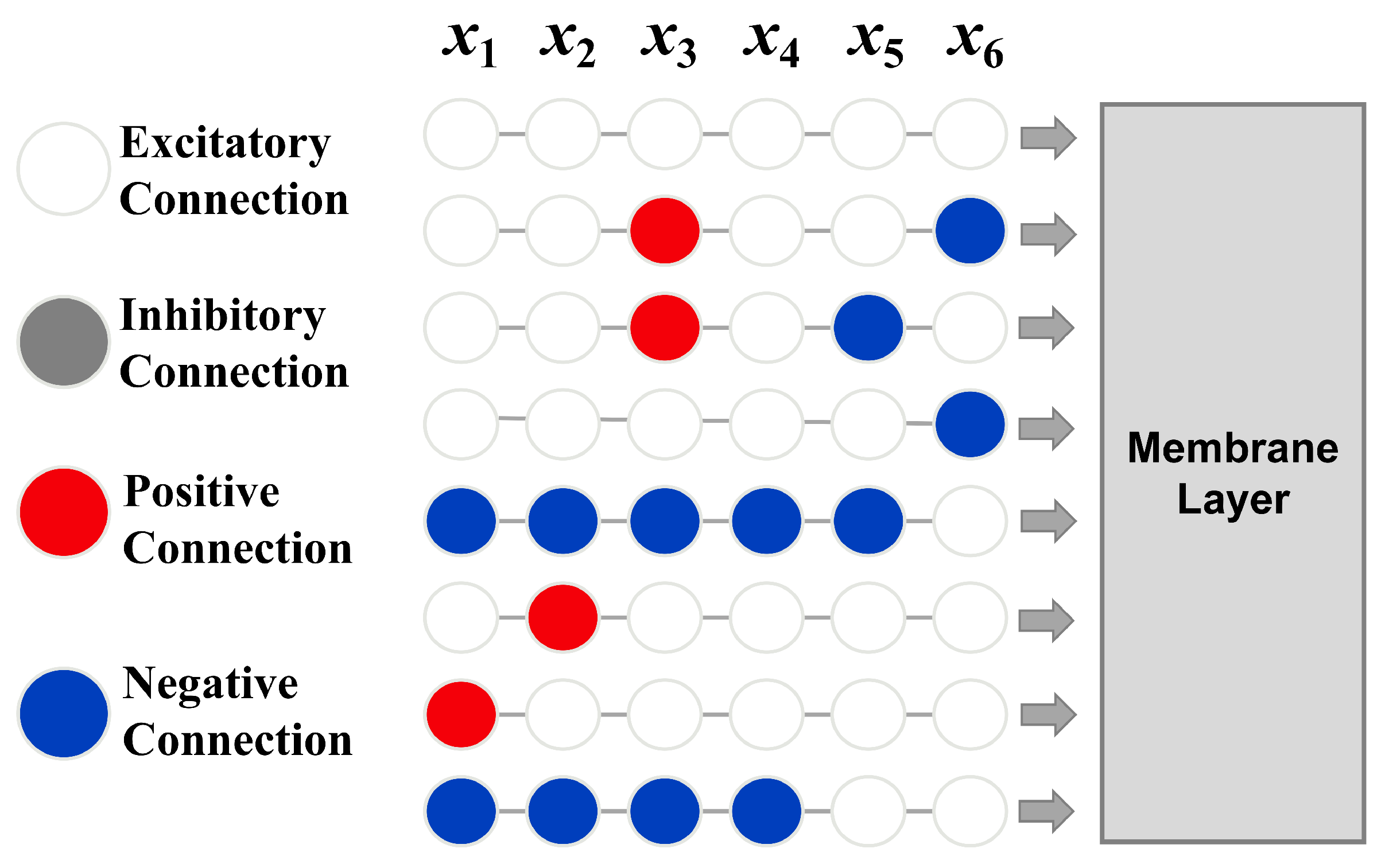
Using the above features to train the DNM model again. Also, the number of dendritic layers was reduced from 10 to 8 due to the reduction of features. The DNM dendritic architecture is obtained as follows in Figure 8.
As can be seen from the Figure 8, there are no features that are all excitatory connections, and there are also no inhibitory connections that represent pruning. At this point, the DNM model is optimal in terms of performance.
The DNM model’s unique construction offers interpretability which sets it apart from other neural networks. This interpretability allows for the effective elimination of unwanted features and facilitates structural tuning. As a result, the DNM model is more adaptable compared to general neural networks.

4.5. Sensitivity Analysis

To evaluate the robustness of the model, this section conducts a sensitivity analysis on the final model. In real-world residential electricity consumption forecasting, many variables are prone to errors. For example, variables such as house area and swimming pool usage time are typically provided by homeowners rather than being measured accurately, and thus may contain certain deviations. Additionally, some errors may also exist during data filtering and construction processes. Therefore, it is necessary to perform a sensitivity analysis on the DNM model.
In this study, we introduced perturbations to the final input dataset of the model to evaluate its sensitivity. Specifically, three random variables were selected from the dataset in each iteration, and perturbations with a magnitude of 0.05 (a commonly used perturbation level) were added. This process was repeated 10 times under the perturbation condition, and the model evaluations were recorded. The detailed results are presented in Table 9.
The mean value of R 2 in the Table 9 is 0.6903, which differs by approximately 0.05 from the model’s performance of 0.7423 without any perturbation. This result indicates that the DNM model’s prediction R 2 variation under noise is within an acceptable range. The model demonstrates good stability and is capable of handling the residential electricity prediction task under data perturbation.

4.6. Practical Significance

The data in this paper comes from the 2020 Residential Energy Consumption Survey, which primarily targets U.S. households. From the final model predictions, it can be seen that Features 2, 3, 4, and 5 are all components of the total electricity consumption. Feature 2 represents electricity usage excluding space heating, space cooling, and refrigerators, and it is undoubtedly closely related to the total electricity consumption. Features 3 and 4 represent the electricity consumption for space cooling and heating, which play a significant role in the total electricity consumption. This indicates that space cooling and heating are major sources of household electricity consumption. Feature 5 corresponds to the electricity consumption for water heating. Given the significant time spent on water usage in daily life, the electricity consumption for water heating contributes notably to the total electricity consumption prediction. The above features are the ones that need to be constructed. There are only two features that do not require construction: the house’s square footage and the months during which the pool was used last year. It is evident that house size is positively correlated with electricity consumption—larger houses tend to consume more electricity. As for the pool’s electricity usage, it is clearly higher than that of any other appliance, even the entire house’s consumption. Therefore, if electricity saving is desired, paying attention to the consumption of space cooling or heating, reducing the frequency of water heating, and limiting the use of the pool can be quite helpful.

5. Summary

5.1. Theoretical and Practical Implementations

This study employs a DNM combined with the AdaMax algorithm to predict residential electricity consumption. As a type of neural network model, the dendritic neural network’s unique structure excellently demonstrates the nonlinear relationships between different features, effectively extracting and utilizing information from housing characteristics, resident activities, and weather features. Additionally, thanks to the DNM’s special self-pruning feature, it not only thoroughly considers the impact of various features during model fitting but also effectively reduces the degree of model overfitting. The model requires setting only a few hyperparameters in advance, such as the learning rate, the number of dendritic layers, and the value of k. Moreover, the use of the AdaMax algorithm allows for automatic updates of the learning rate during operation, further minimizing the impact of hyperparameters on the model.
From a practical application perspective, the dendritic neural network model can accurately predict residential electricity consumption with simple social statistics. Furthermore, the developed DNM can be easily applied to simulate regional or even national electricity demand across various scenarios of building characteristics, occupant characteristics and behavior. Due to the current limitations of DNM in handling high-dimensional data, future research will focus on how to prevent gradient explosion and vanishing gradients in DNM, as well as how to handle high-dimensional data effectively. The features excluded in this paper are not necessarily useless; they may be more fully utilized in future DNM models.

5.2. Conclusions

This paper proposes the integration of the DNM with the AdaMax algorithm for predicting residential electricity consumption. As technological advancements and population growth increase, so does humanity’s demand for energy. However, significant energy consumption leads to the depletion of natural resources and environmental pollution. Therefore, reducing energy consumption is essential for sustainable development. Residential electricity consumption constitutes a significant portion of total energy use. Thus, this study aims to predict residential electricity consumption to explore specific energy uses.
The dataset in this study includes 799 features, with 330 features that can be used directly, 468 that require preprocessing, and one target variable to be predicted: residential electricity consumption. For the 330 directly usable features, those with correlations above 0.9 were first removed. Then, Random Forest and XGBoost models were used for cyclic filtering. Each model selecting five features. After removing duplicates, seven features were retained. Among the 468 indirectly used features, the five features were filtered by Random Forest, which provided reference for feature construction. XGBoost was used to fit the five filtered features that could not be used directly. The predicted values of XGBoost were used as new features to be retained. The final retained dataset is twelve features, include 7 directly used features and 5 indirectly used features. The dataset was split into a training set and a test set at a ratio of 7:3.
The DNM is a specialized neural network with a unique structure and self-pruning capabilities, offering better interpretability and some degree of overfitting prevention compared to other neural networks. It also has fewer hyperparameters, contributing to more stable operation. The DNM’s hyperparameters include the number of epochs, k value, number of dendritic layers, and initial learning rate. More epochs generally increase model accuracy, and due to its self-pruning feature, overfitting is less of a concern within certain limits. Thus, the number of epochs was set to 1500.
Since the AdaMax algorithm updates the learning rate during operation, the initial learning rate has a minimal impact on the model. Bayesian optimization was used to tune the DNM. The optimal parameters obtained through Bayesian optimization included a k value of 1.4, an initial learning rate of 0.0054, and 15 dendritic layers.
In this paper, we compare the performance of the DNM with five other models: XGBoost, ANN, LightGBM, Transformer and SVM. The R 2 of the DNM is 0.7405. The results show that the DNM surpasses these models in terms of higher R 2 and lower MSE and MAE, indicating its superior suitability for predicting residential electricity consumption.
In this paper, the DNM model is distinguished from other neural network models by being interpretable, filtered again for features, and simply adjusted for structure. It makes the DNM model improve the R 2 from 0.74 to 0.742 with fewer features and simpler structure.

Author Contributions

Conceptualization, T.J.; methodology, T.J., R.X. and K.S.; software, R.X.; validation, T.J., R.X., K.S. and J.G.; formal analysis, T.J. and R.X.; investigation, R.X. and K.S.; resources, T.J.; data curation, R.X.; writing—Original Draft, T.J.; writing—Review and Editing, T.J., R.X., K.S. and J.G.; visualization, R.X.; supervision, T.J.; project administration, T.J.; funding acquisition, T.J. All authors have read and agreed to the published version of the manuscript.

Funding

This research was partially supported by the National Natural Science Foundation of China (No. 12201304). This work is also supported by the General Research Projects of Philosophy and Social Sciences in Colleges and Universities (2022SJYB0140).

Data Availability Statement

In this study, data were collected from the 2020 Residential Energy Consumption Survey at https://www.eia.gov/consumption/residential, accessed on 26 December 2024.

Conflicts of Interest

The authors declare that there are no conflict of interests.

Abbreviations

The following abbreviations are used in this manuscript:
DNMdendritic neural network-based model
ANNArtificial Neural Network
SVMSupport Vector Machine
MSEMean Squared Error
MAEMean Absolute Error

Appendix A

The scatter plots presented in this appendix show the relationship between the predictor variable (residential electricity consumption) and other dependent variables.
Figure A1. The relationship between the predictor variable (residential electricityconsumption) and other dependent variables. (a) Scatter plot of BEDROOMS; (b) BTUNGPLHEAT; (c) ELWATER; (d) FUELHEAT; (e) KWHCOL; (f) KWHOTH; (g) KWHSPH; (h) KWHWTH; (i) MONPOOL; (j) SQFTEST; (k) TOTHSQFT; (l) TYPEHUQ.
Mathematics 13 00575 g0a1aMathematics 13 00575 g0a1b

References

  1. Wikipedia Contributors. World Energy Consumption. Wikipedia. 2024. Available online: https://en.wikipedia.org/wiki/World_energy_consumption (accessed on 30 July 2024).
  2. Stocker, T. Climate Change 2013: The Physical Science Basis: Working Group I Contribution to the Fifth Assessment Report of the Intergovernmental Panel on Climate Change; Cambridge University Press: Cambridge, UK, 2014. [Google Scholar]
  3. Lopes, M.A.R.; Antunes, C.H.; Reis, A.; Martins, N. Estimating energy savings from behaviours using building performance simulations. Build. Res. Inf. 2017, 45, 303–319. [Google Scholar] [CrossRef]
  4. IEA Energy Efficiency. Buildings; International Energy Agency: Paris, France, 2018.
  5. Lertpalangsunti, N.; Chan, C.W. An architectural framework for the construction of hybrid intelligent forecasting systems: Application for electricity demand prediction. Eng. Appl. Artif. Intell. 1998, 11, 549–565. [Google Scholar] [CrossRef]
  6. Filippini, M.; Pachauri, S. Elasticities of electricity demand in urban Indian households. Energy Policy 2004, 32, 429–436. [Google Scholar] [CrossRef]
  7. Guo, Z.; Zhou, K.; Zhang, C.; Lu, X.; Chen, W.; Yang, S. Residential electricity consumption behavior: Influencing factors, related theories and intervention strategies. Renew. Sustain. Energy Rev. 2018, 81, 399–412. [Google Scholar] [CrossRef]
  8. Van den Brom, P.; Hansen, A.R.; Gram-Hanssen, K.; Meijer, A.; Visscher, H. Variances in residential heating consumption–Importance of building characteristics and occupants analysed by movers and stayers. Appl. Energy 2019, 250, 713–728. [Google Scholar] [CrossRef]
  9. Borozan, D. Regional-level household energy consumption determinants: The European perspective. Renew. Sustain. Energy Rev. 2018, 90, 347–355. [Google Scholar] [CrossRef]
  10. Zou, P.X.W.; Xu, X.; Sanjayan, J.; Wang, J. Review of 10 years research on building energy performance gap: Life-cycle and stakeholder perspectives. Energy Build. 2018, 178, 165–181. [Google Scholar] [CrossRef]
  11. Zou, P.X.W.; Xu, X.; Sanjayan, J.; Wang, J. A mixed methods design for building occupants’ energy behavior research. Energy Build. 2018, 166, 239–249. [Google Scholar] [CrossRef]
  12. Amasyali, K.; El-Gohary, N.M. A review of data-driven building energy consumption prediction studies. Renew. Sustain. Energy Rev. 2018, 81, 1192–1205. [Google Scholar] [CrossRef]
  13. Gao, F.; Shao, X. Electricity consumption prediction based on a dynamic decomposition-denoising-ensemble approach. Eng. Appl. Artif. Intell. 2024, 133, 108521. [Google Scholar] [CrossRef]
  14. Ghimire, S.; Deo, R.C.; Casillas-Pérez, D.; Salcedo-Sanz, S.; Pourmousavi, S.A.; Acharya, U.R. Probabilistic-based electricity demand forecasting with hybrid convolutional neural network-extreme learning machine model. Eng. Appl. Artif. Intell. 2024, 132, 107918. [Google Scholar] [CrossRef]
  15. Do, H.; Cetin, K.S. Residential building energy consumption: A review of energy data availability, characteristics, and energy performance prediction methods. Curr. Sustain./Renew. Energy Rep. 2018, 5, 76–85. [Google Scholar] [CrossRef]
  16. Biswas, M.A.R.; Robinson, M.D.; Fumo, N. Prediction of residential building energy consumption: A neural network approach. Energy 2016, 117, 84–92. [Google Scholar] [CrossRef]
  17. Kaytez, F.; Taplamacioglu, M.C.; Cam, E.; Hardalac, F. Forecasting electricity consumption: A comparison of regression analysis, neural networks and least squares support vector machines. Int. J. Electr. Power Energy Syst. 2015, 67, 431–438. [Google Scholar] [CrossRef]
  18. McLoughlin, F.; Duffy, A.; Conlon, M. Characterising domestic electricity consumption patterns by dwelling and occupant socio-economic variables: An Irish case study. Energy Build. 2012, 48, 240–248. [Google Scholar] [CrossRef]
  19. Bedir, M.; Hasselaar, E.; Itard, L. Determinants of electricity consumption in Dutch dwellings. Energy Build. 2013, 58, 194–207. [Google Scholar] [CrossRef]
  20. O’Neill, B.C.; Chen, B.S. Demographic determinants of household energy use in the United States. Popul. Dev. Rev. 2002, 28, 53–88. [Google Scholar]
  21. Hansen, A.R. The social structure of heat consumption in Denmark: New interpretations from quantitative analysis. Energy Res. Soc. Sci. 2016, 11, 109–118. [Google Scholar] [CrossRef]
  22. Keynia, F. A new feature selection algorithm and composite neural network for electricity price forecasting. Eng. Appl. Artif. Intell. 2012, 25, 1687–1697. [Google Scholar] [CrossRef]
  23. Foster, V.; Tre, J.-P.; Wodon, Q. Energy Consumption and Income: An Inverted-U at the Household Level; The World Bank: Washington, DC, USA, 2000. [Google Scholar]
  24. Dong, B.; Cao, C.; Lee, S.E. Applying support vector machines to predict building energy consumption in tropical region. Energy Build. 2005, 37, 545–553. [Google Scholar] [CrossRef]
  25. Tso, G.K.F.; Yau, K.K.W. Predicting electricity energy consumption: A comparison of regression analysis, decision tree and neural networks. Energy 2007, 32, 1761–1768. [Google Scholar] [CrossRef]
  26. Pino, R.; Parreno, J.; Gomez, A.; Priore, P. Forecasting next-day price of electricity in the Spanish energy market using artificial neural networks. Eng. Appl. Artif. Intell. 2008, 21, 53–62. [Google Scholar] [CrossRef]
  27. Wang, Y.; Yu, Y.; Zhang, T.; Song, K.; Wang, Y.; Gao, S. Improved dendritic learning: Activation function analysis. Inf. Sci. 2024, 2024, 121034. [Google Scholar] [CrossRef]
  28. Yu, Y.; Wang, Y.; Gao, S.; Tang, Z. Statistical modeling and prediction for tourism economy using dendritic neural network. Comput. Intell. Neurosci. 2017, 2017, 7436948. [Google Scholar] [CrossRef]
  29. Gao, S.; Zhou, M.; Wang, Y.; Cheng, J.; Yachi, H.; Wang, J. Dendritic neuron model with effective learning algorithms for classification, approximation, and prediction. IEEE Trans. Neural Netw. Learn. Syst. 2018, 30, 601–614. [Google Scholar] [CrossRef]
  30. Sadoun, A.M.; Najjar, I.M.R.; Fathy, A.; Abd Elaziz, M.; Al-qaness, M.A.A.; Abdallah, A.W.; Elmahdy, M. An enhanced Dendritic Neural Algorithm to predict the wear behavior of alumina coated silver reinforced copper nanocomposites. Alex. Eng. J. 2023, 65, 809–823. [Google Scholar] [CrossRef]
  31. Brochu, E.; Cora, V.M.; De Freitas, N. A tutorial on Bayesian optimization of expensive cost functions, with application to active user modeling and hierarchical reinforcement learning. arXiv 2010, arXiv:1012.2599. [Google Scholar]
Figure 1. Architecture of DNM model.
Mathematics 13 00575 g001
Figure 3. Flowchart of variable selection and construction.
Mathematics 13 00575 g003
Figure 4. Architecture of DNM dendritic layer.
Mathematics 13 00575 g004
Figure 5. Bar chart comparing R 2 of different models.
Mathematics 13 00575 g005
Figure 6. Bar chart comparing R 2 of model training and test sets at different Max Depths.
Mathematics 13 00575 g006
Figure 7. Cyclic screening comparison R 2 line chart.
Mathematics 13 00575 g007
Figure 8. Architecture of DNM dendritic layer.
Mathematics 13 00575 g008
Table 1. Final Selected Feature Table.
FeatureLabelDescriptionVariable Value RangeData Acquisition
BTUHEATFeature 1Calibrated natural gas usage for swimming pool heaters, in thousand Btu0–183,303.25Construction
KWHOTHFeature 2Calibrated electricity usage for end uses other than space heating, space cooling, water heating, and refrigerators, in kilowatt-hours15.51–175,602.87Construction
KWHSPHFeature 3Calibrated electricity usage for space heating, main and secondary, in kilowatt-hours0–49,544.4Construction
KWHCOLFeature 4Calibrated electricity usage for space cooling, in kilowatthours0–31,758.14Construction
KWHWTHFeature 5Calibrated electricity usage for water heating, main and secondary, in kilowatthours0–25,824.46Construction
FUELHEATFeature 6Main space heating fuel5 Electricity; 1 Natural gas; 2 Propane; 3 Fuel oil; 7 Wood; –2 Not applicableDirectly obtained
TOTHSQFTFeature 7Square footage of the housing unit that is heated by space heating equipment0–15,000Directly obtained
SQFTESTFeature 8Respondent-reported square footage240–15,000Directly obtained
TYPEHUQFeature 9Type of housing unit1 Mobile home; 2 Single-family house detached from any other house; 3 Single-family house attached to houses; 4 Apartment in a building with 2 to 4 units; 5 Apartment in a building with 5 or more unitsDirectly obtained
MONPOOLFeature 10Months swimming pool used past year0–12; –2 Not applicableDirectly obtained
ELWATERFeature 11Electricity used for water heating; a derived variable1 Yes; 0 NoDirectly obtained
BEDROOMSFeature 12Number of bedrooms0–6Directly obtained
Table 2. Optimal Hyperparameters of the Models.
ModelOptimal Hyperparameters
Random Forest‘max depth’: 16,‘max features’: 0.82718, ‘min samples leaf’: 1,‘min samples split’: 2,‘n estimators’: 442.
ANN‘alpha’: 0.00303, ‘hidden layer sizes’: 23, ‘learning rate init’: 0.00932.
SVM‘C’: 29.897940495479673, ‘epsilon’ : 0.3916592230820964, ‘gamma’: 0.01.
Transformer‘model dim’: 64,‘num heads’: 8‘num layers’: 2.
XGBoost‘learning rate’: 0.04857, ‘max depth’: 5, ‘n estimators’: 819, ‘reg alpha’: 0.32945, ‘reg lambda’: 0.82747.
LightGBM‘learning rate’: 0.06107, ‘colsample bytree’: 0.5, ‘min child samples’: 10, ‘n estimators’: 207, ‘num:leaves’: 20, ‘reg alpha’: 0.40235, ‘reg lambda’: 0.0, ‘subsample’: 0.5.
Table 3. The Model performance on the Test Set.
ModelMSEMAE R 2
DNM12,316,995.02384.860.7405
XGBoost12,711,146.422414.840.7286
ANN14,575,288.02612.320.6888
LigthGBM14,831,064.052624.930.6833
Transformer14,991,023.02661.800.6799
SVM15,421,989.192628.010.6707
Table 4. Model runtime comparison table.
ModelRuntime
XGBoost0.296 s
LigthGBM0.646 s
ANN6.27 s
SVM16.7 s
DNM434 s
Transformer602 s
Table 5. Comparison table of results from different optimization algorithms.
Optimization Algorithms R 2
Adamax0.7401
Adam0.7401
Adagrad0.7361
SGD0.7264
Table 6. The number of connections of each type.
Feature LabelExcitatory ConnectionInhibitory ConnectionPositive ConnectionNegative Connection
Feature 18200
Feature 22107
Feature 33214
Feature 43016
Feature 54006
Feature 610000
Feature 78002
Feature 86202
Feature 97030
Feature 106004
Feature 117012
Feature 127003
Table 7. The feature importance scores of the features.
Feature LabelFeature Importance
Feature 11
Feature 27.5
Feature 36
Feature 47
Feature 56
Feature 60
Feature 72
Feature 83
Feature 93
Feature 102
Feature 113
Feature 123
Table 8. Final Selected Feature Table.
FeatureLabelDescriptionData Acquisition
KWHOTHFeature 2Calibrated electricity usage for end uses other than space heating, space cooling, water heating, and refrigerators, in kilowatt-hoursConstruction
KWHSPHFeature 3Calibrated electricity usage for space heating, main and secondary, in kilowatt-hoursConstruction
KWHCOLFeature 4Calibrated electricity usage for space cooling, in kilowatthoursConstruction
KWHWTHFeature 5Calibrated electricity usage for water heating, main and secondary, in kilowatthoursConstruction
SQFTESTFeature 8Respondent-reported square footageDirectly obtained
MONPOOLFeature 10Months swimming pool used past yearDirectly obtained
Table 9. Robustness Evaluation Table for DNM Model with 0.05 Perturbation.
Times12345678910
R 2 0.69070.69170.69100.69250.68860.69120.69010.68790.68860.6907
Disclaimer/Publisher’s Note: The statements, opinions and data contained in all publications are solely those of the individual author(s) and contributor(s) and not of MDPI and/or the editor(s). MDPI and/or the editor(s) disclaim responsibility for any injury to people or property resulting from any ideas, methods, instructions or products referred to in the content.