Article

Euler–Riemann–Dirichlet Lattices: Applications of η(s) Function in Physics

by
Hector Eduardo Roman
Department of Physics, University of Milano-Bicocca, Piazza della Scienza 3, 20126 Milano, Italy
Mathematics 2025, 13(4), 570; https://doi.org/10.3390/math13040570
Submission received: 2 January 2025 / Revised: 3 February 2025 / Accepted: 6 February 2025 / Published: 9 February 2025
(This article belongs to the Section E4: Mathematical Physics)

Abstract

:
We discuss applications of the Dirichlet η ( s ) function in physics. To this end, we provide an introductory description of one-dimensional (1D) ionic crystals, which are well-known in the condensed matter physics literature, to illustrate the central issue of the paper: A generalization of the Coulomb interaction between alternating charges in such crystalline structures. The physical meaning of the proposed form, characterized by complex (in the mathematical sense) ion–ion interactions, is argued to have emerged in many-body systems, which may include effects from vacuum energy fluctuations. We first consider modifications to the bare Coulomb interaction by adding an imaginary component to the exponent of the Coulomb law of the form s = 1 + i b , where b is a real number. We then extend the results to slower-decaying interactions, where the exponent becomes s = a + i b , presenting numerical results for values 1 / 2 a 2 , which include the critical strip relevant to the Riemann hypothesis scenario.

1. Introduction

The Riemann hypothesis, which conjectures that the non-trivial zeros of the Riemann ζ ( s ) function, ζ ( 1 / 2 ± i μ n ) = 0 , occur solely for real values of μ n , has sparked considerable interest not just among mathematicians specializing in number theory but also in a wide range of scientific disciplines, including physics, which is the focus of this paper. The applications of the ζ ( s ) function in physics are numerous and have been thoroughly reviewed in [1]. To provide an overview of the current status of the field, we briefly review recent works that are relevant to our discussions. We begin with the physical applications.
The connections between the properties of ζ ( s ) , including the Riemann hypothesis, and scattering amplitudes in quantum field theory are explored in [2]. A relationship between ζ ( s ) and a physical system, known as the Hilbert–Pólya conjecture, was proposed in the early 1900s, suggesting that μ n could be interpreted as the eigenvalues of some quantum mechanical Hamiltonian. Since then, significant efforts have been devoted to identifying such an operator or uncovering other links to physics. In this context, the author constructs a closed-form scattering amplitude, revealing the remarkable result that real ‘masses’ μ n are consistent with the Riemann hypothesis.
Various physical problems related to the Riemann hypothesis have been reviewed in [3], including the Hilbert–Pólya conjecture, connections to random matrix theory, the relationship with the Lee–Yang theorem on the zeros of the partition function, and phase transitions, as well as topics such as random walks, billiards, and more.
Numerical series of prime numbers can be generated as sequences of points in a 1D lattice occupied by electric charges [4]. Based on this mapping, a single-particle Hamiltonian model is proposed for the distribution of primes ρ ( n ) along the x-axis, which are treated as quantum particles located at stationary points, x n , of a Lennard-Jones-like potential. A particle-counting function, π Q ( x ) , analogous to the prime-counting function, π ( x ) , is defined and obtained with the help of the Hellmann–Feynman theorem. The conditions on the sequence of energy eigenvalues, E ( n ) , for the system to ensure that the Riemann hypothesis holds for π Q ( x ) , are derived.
An alternative approach to the prime-counting function π ( x ) involves a connection between the distribution of the zeros of ζ ( s ) and the poles of the scattering matrix S of a quantum system. Arguments are presented in [5]. They are aimed at explaining the still unresolved question of why the poles and zeros of the S-matrix of an ideal system, which could potentially satisfy the Riemann hypothesis, always occur in pairs and are related by complex conjugation. This result thus suggests a potential pathway toward a proof of the Riemann conjecture.
A novel formulation of the zeta function represented as the sum of an infinite series of delta and cosine functions is studied in [6]. The formula exhibits duality properties, establishing a link between the Riemann hypothesis and the new formulation. Furthermore, the quantum behaviors of the energy and eigenstates for this new mathematical model are examined, offering valuable insights into several key physical phenomena, including the collapse of the wavefunction during measurement, quantum entanglement, and double-slit experiments.
An introduction to the Riemann hypothesis using familiar mathematical techniques is presented in [7], providing useful heuristic arguments in support of the hypothesis. The latter is shown to be connected to quantum mechanics by interpreting the Dirichlet series as a superposition of probability amplitudes, which leads to a unique potential with a logarithmic energy spectrum.
Other aspects of interest for our discussions include the question of non-Hermitian Hamiltonians, quantum dissipative systems, and the case of complex interactions in many-body systems. We briefly illustrate these different issues with some examples.
A nonlinear field theory, which describes frictional effects in dissipative systems through a Schrödinger-type field equation with a logarithmic nonlinearity, has become a paradigm in the field [8]. The nonlinear field equation for the damped harmonic oscillator can be solved exactly, showing that wavefunctions and a wavepacket-like solution with a Gaussian shape display reasonable physical properties that differ from those of the undamped case. Properties of the nonlinear friction term are examined and compared to similar terms used by other authors. Finally, a nonlinear friction term equivalent to the logarithmic nonlinearity is obtained but expressed in terms of combinations of position and linear momentum operators, along with their mean values.
A purely field-based description of matter, represented by well-defined elementary densities rather than by classical fields and point particles, allows for overcoming the present nonphysical divergences in gravitational and Coulomb self-energy [9]. In this approach, the gravitational mass is linked to the real part of the integral of the complex densities of matter, while the electric charge is related to the imaginary part of the same spatial integral in such a way that the field laws would not break down at small distances.
A detailed review of the foundations and applications of non-Hermitian classical and quantum physics has recently become available [10]. Key theorems and fundamental concepts in non-Hermitian linear algebra, such as the Jordan normal form, biorthogonality, exceptional points, pseudo-Hermiticity, and parity-time symmetry, are presented in an accessible and mathematically rigorous way.
It is well known that the Hermitian condition for a Hamiltonian, H = H , is sufficient to ensure a real energy spectrum and unitary time evolution. However, the requirement of Hermiticity is not essential to achieve these properties in general [11]. Actually, it is possible to describe natural processes using non-Hermitian Hamiltonians where the Hermiticity condition can be replaced by a more physically intuitive condition of parity-time (PT) symmetry, H = H P T , without violating any fundamental principles of quantum mechanics. When a Hamiltonian satisfies this relation, it is referred to as PT-symmetric.
From the early days of quantum mechanics, numerous heuristic attempts to model dissipative phenomena in nuclear, atomic, and molecular physics have relied on effective non-Hermitian Hamiltonians. In the past two decades, the introduction of parity-time (PT) symmetry has opened the door for a more systematic exploration of non-Hermitian physics. It is now understood that non-Hermitian Hamiltonians can be rigorously justified, as in the case in which the system dynamics is confined either to a subspace or within the framework of quantum measurement theory, by conditioning quantum trajectories on specific measurement outcomes [12].
To conclude this brief review, we draw the attention of the reader to recent works dealing with the mathematical aspects of the Riemann hypothesis. In [13], new sums over the primes of non-principal Dirichlet characters, which exhibit a conjectured random walk behavior, have been derived. It is shown that the Euler product formula for their L-functions holds to the right of the critical line ( ( s ) > 1 / 2 ), which implies that the Riemann hypothesis is valid for this class of L-functions. From these findings, a new algorithm is proposed for calculating very high Riemann zeros and computing the googol-th ( 10 100 -th) zero to over 100 digits, which surpasses current computational limits.
The approach discussed in [14] involves an analytical study of the functional equation of ζ ( s ) based on a complex function, which is treated as a real function of two real variables, and its modulus, alongside extensive numerical analysis to support the Riemann hypothesis within the computational resources. These findings offer a new mathematical perspective on assessing the validity of Riemann’s hypothesis. Finally, a novel approach to the Riemann hypothesis, emphasizing the relationship between prime gaps and the non-trivial zeros of the Riemann zeta function, has been discussed recently [15]. The key findings are that past non-trivial zeros may predict future prime gaps; nonlinear interactions between prime gaps and non-trivial zeros are present; and intricate feedback loops between the two may exist. These insights open new avenues for future mathematical exploration.
In this work, we investigate potential applications of the Riemann ζ ( s ) function formalism, particularly in relation to the Dirichlet η ( s ) function, within condensed matter physics. While a similar problem is briefly discussed in [1], our model introduces, to the best of our knowledge, several novel features making it a valuable contribution for readers interested in ongoing discussions surrounding the Riemann hypothesis in a broader context.
Our work builds on well-established results from condensed matter physics on the cohesive energy in ionic crystals [16,17,18,19]. We focus on the one-dimensional case of an infinite ionic chain with alternating electric charges. In addition to the Coulomb interaction, we use the Born exponential form for the repulsive core between neighboring ions, which prevents the lattice from collapsing, as opposed to a Lennard-Jones type, since in ionic systems, such as alkali halides, the charge transfer from the alkali atom to the halide atom is incomplete, which leads to a partially closed shell of outer electrons.
This work is motivated by the following physical considerations concerning many-body interactions in strongly coupled electron-ion systems. In real materials, it is anticipated that interactions beyond the fundamental Coulomb force between charges may become significant. Specifically, the repulsive short-range interaction arises from an interplay of electrostatic and quantum mechanical effects, such as the Pauli exclusion principle. At medium-range distances, induced dipole–dipole (van der Waals) interactions can become significant, while electron–phonon couplings may also contribute to anomalies in the structural properties of materials. In addition to these interactions, phenomena related to vacuum polarization and self-energy effects on electrons may also play a crucial role in determining the system’s stability in certain conditions.
To account for these complex scenarios in a straightforward manner, we propose introducing an effective Coulomb (EC) interaction, V EC ( r ) , between charges separated by a distance r, which leads to the following
CONJECTURE : V EC ( r ) = ± V 0 1 r s , with s = a + i b .
Here, both a and b are real numbers. To illustrate how the effective interaction V EC ( r ) actually works, we apply it to the ionic chain described above because it admits an exact solution. Applications to real systems go beyond the scope of the present work. We then show that the total energy per site of the chain can be written as,
E T ( a 0 , s ) = A c a 0 ( s ) [ η ( s ) ] ,
where A is a dimensionless quantity and a 0 ( s ) is the lattice constant at equilibrium. Here, we first consider the case a = 1 and b > 0 , which reduces to the bare Coulomb limit when b = 0 , and then present some results for the broader case, 1 / 2 a 2 , which covers the critical strip.
The paper is organized as follows. In Section 2, we review the connection of η ( s ) to ζ ( s ) . In Section 3, we define our lattice of charges and revisit the main results for a standard one-dimensional ionic crystal in Section 3.1. Section 3.2 introduces the Euler–Riemann–Dirichlet (ERD) lattice model, which uses η ( s ) to generalize the Coulomb law. We discuss the implications of this new interaction in detail, providing plausibility arguments for the physical mechanism behind the complex interaction, which includes imaginary components. In Section 4, we present ERD results at and near the critical strip, comparing them with those from the previous section. In addition, we include three appendices: The first, in Appendix A, discusses the properties of the η ( s ) function. The second, in Appendix B, covers prime numbers, presenting both numerical and analytical results that extend previous literature. The third, in Appendix C, considers the critical strip of the Riemann zeta function, where the behavior of the non-trivial zeros of ζ ( s ) is examined. Finally, our concluding remarks are presented in Section 5.

2. The Function η ( s ) and Its Relation to ζ ( s )

Leonhard Euler was fascinated by infinite numerical series [20]. This culminated in 1735 while in Saint Petersburg, when he published the solution to the famous Basel problem, n = 1 n 2 = π 2 / 6 . One hundred years later, Bernhard Riemann generalized this class of series to the complex plane by defining the function [21]
ζ ( s ) = n = 1 1 n s , with s = a + i b ,
where both ( a , b ) R . This is now known as the Riemann zeta function. We note that, in standard notation, a = σ and b = t . The complex function ζ ( s ) in Equation (3) is absolutely convergent when a > 1 with a single pole at s = 1 and residue 1 (see below). In [21], Riemann showed that ζ ( s ) satisfies the functional equation (see the discussion in [20], and also the detailed monograph in [22]),
ζ ( s ) = π s 1 / 2 Γ ( { 1 s } / 2 ) Γ ( s / 2 ) ζ ( 1 s ) .
Equation (4) allows one to obtain ζ ( s ) for a < 0 , from ζ ( 1 s ) with 1 s = 1 + | a | i b . In particular, note that when a = 2 m for integer m > 0 , Equation (4) gives the so-called trivial zeros of the Riemann zeta function, ζ ( 2 m ) = 0 , due to the simple poles of Γ ( s / 2 ) at s / 2 = m , with residues ( 1 ) m / m ! . The next question is how to calculate ζ ( s ) within the range 0 a 1 , also known as the critical strip, which brings us to the central issue of this paper.
For this purpose, the alternating Riemann zeta function, commonly known as the Dirichlet eta function, is emphasized,
η ( s ) = n = 1 ( 1 ) n 1 n s ,
which converges for ( s ) = a > 0 . It can be shown that η ( s ) is proportional to ζ ( s ) ,
η ( s ) = 1 2 1 s ζ ( s ) ,
thus allowing us to evaluate ζ ( s ) over the entire range 0 a 1 , except at s = 1 ( a = 1 , b = 0 ) where the simple pole is located, while the value η ( 0 ) = 1 / 2 can be derived using the functional relation Equation (4) (see Appendix A and [23] for details). As a result, Equation (6) yields ζ ( 0 ) = 1 / 2 , and using the value η ( 1 ) = log 2 , one finds ζ ( s ) = 1 / ( s 1 ) for s 1 .
Another important result derived from Equation (6) is that η ( s ) should have simple zeros, s m , when the factor 1 2 1 s m = 0 , which is consistent with the single simple pole of ζ ( s ) at s = 1 . This yields
η ( s m ) = 0 , with s m = 1 + i 2 π m log 2 ,
for integer m 0 . Efficient algorithms have been designed to calculate ζ ( s ) for generic s (see, for instance, [24]).

3. Euler–Riemann–Dirichlet Lattices

In Section 3.1, we provide an overview of the known results for standard 1D ionic lattices, offering the reader the necessary background for developing a more general model in Section 3.2. The latter is proposed to describe lattices with many-body interactions between ions, referred to as Euler–Riemann–Dirichlet (ERD) lattices.

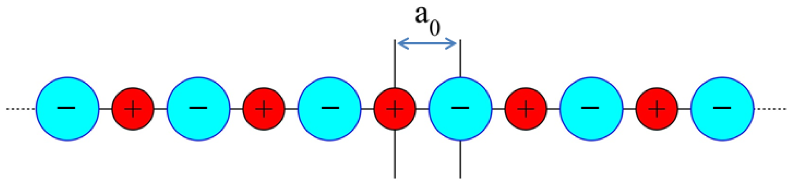
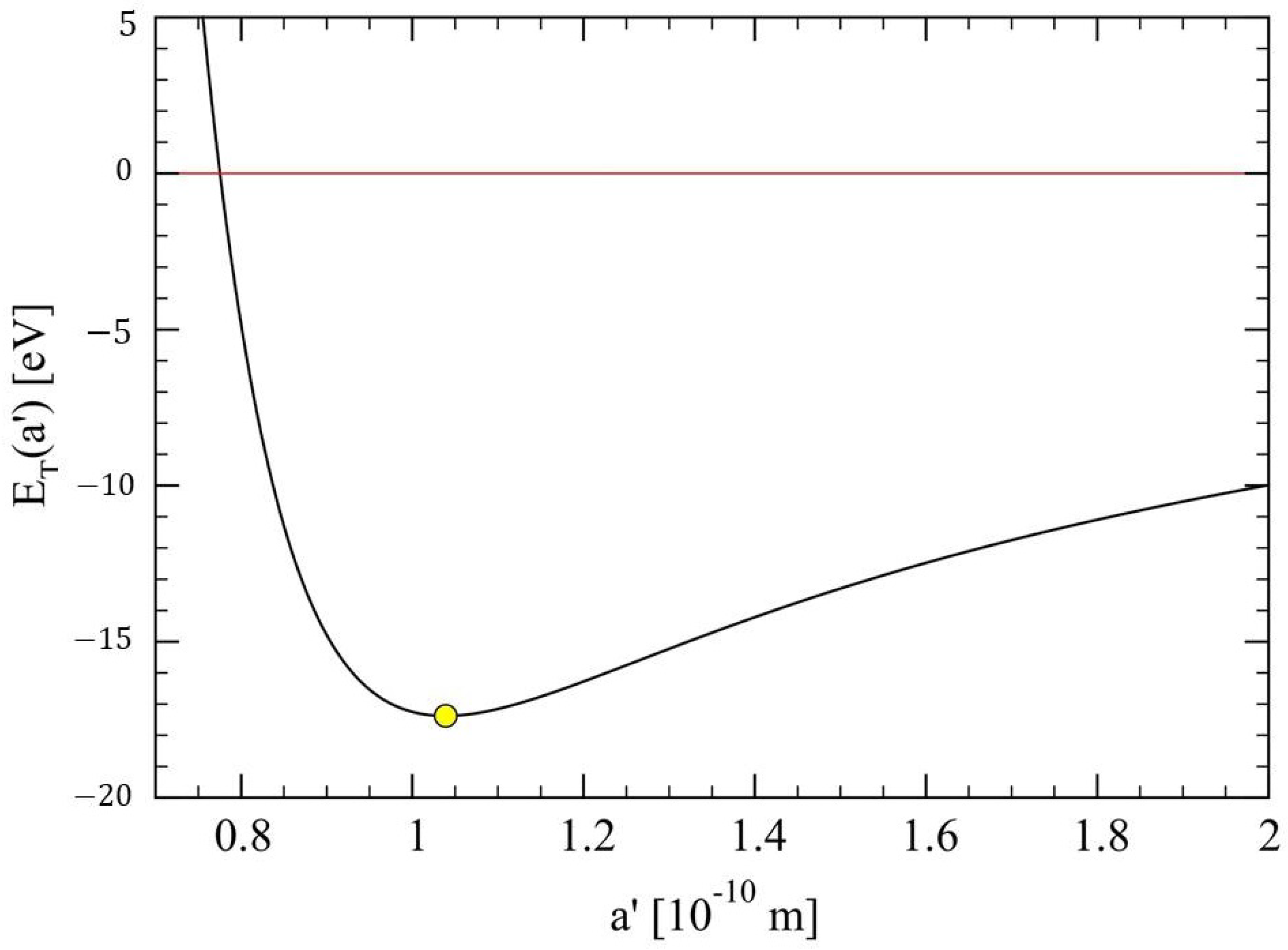
3.1. Standard Ionic Lattices

To illustrate applications of the functions defined in Section 1, we begin by considering a one-dimensional ionic crystal, where the ions are arranged alternately as shown in Figure 1. In addition to the Coulomb interaction, we assume the presence of a short-range repulsive force that prevents the lattice from collapsing [16,19]. At equilibrium, the total Coulomb energy acting on a reference ion is exactly balanced by the short-range forces between the ion and its two nearest neighbors. Let us specify these forces in detail.
We consider the reference ion (index 0 and positive charge q I ) to be located at the origin of coordinates, x 0 = 0 , and the remaining ions at x j = j a 0 , with | j | 1 , carrying charges ( 1 ) j q I . The Coulomb interaction energy between the reference ion and the one at x j is given by
E 0 j C = q I 2 4 π ϵ 0 ( 1 ) j 1 | x j | , | j | 1 .
For convenience, we define, q I = ± q e , where q is a positive real number, e is the unit of electric charge, n = | j | , | x j | = n a 0 , and the fine-structure constant α 0 = e 2 / ( 4 π ϵ 0 c ) 1 / 137 . Therefore, denoting E C ( n ) E 0 j C , Equation (8) becomes,
E C ( n ) = α 0 q 2 c a 0 ( 1 ) n 1 n , n 1 .
The repulsive interaction energy is modeled using the Born exponential form [16],
E R ( n ) = E 0 e n a 0 / ρ , for n = 1 ,
and for the remaining terms, n > 1 , we assume E R ( n ) = 0 , since their contribution is negligible because in most physical cases, ρ a 0 . There are other forms for E R known in the literature involving short-range power-law repulsions say, E R E 0 ( ρ / a 0 ) m R , with m R 12 for a Lennard-Jones type of interaction energy typical of noble gases. We stick at the Born shape in this work for simplicity (see also the discussion on this matter in [19]).
The total lattice energy per site, E T , is just the sum over all ion positions, which takes the form
E T = 2 n = 1 [ E R ( n ) + E C ( n ) ] = 2 E 0 e a 0 / ρ 2 α 0 q 2 c a 0 n = 1 ( 1 ) n 1 n ,
where we recognize the Dirichlet function η ( 1 ) = log 2 in the last term (Equation (5)).
Now, the condition of equilibrium requires a stable minimum, i.e., E T / a | a 0 = 0 , and 2 E T / a 2 | a 0 > 0 , yielding
E T / a | a 0 = 0 a 0 2 e a 0 / ρ = α 0 q 2 η ( 1 ) c ρ E 0 ,
and
2 E T / a 2 | a 0 = 2 α 0 q 2 η ( 1 ) c ρ a 0 2 1 2 ρ a 0 > 0 ,
while the total energy per site at the minimum becomes,
E T ( a 0 ) = 2 α 0 q 2 η ( 1 ) c a 0 1 ρ a 0 < 0 .
To obtain a 0 , Equation (12) must be solved numerically. It is convenient to consider an example to get an idea of the order of magnitude of the quantities involved, as illustrated in Figure 2. To be noted is that the interaction energies between nearest-neighbor ions give already the right order of magnitude for the total lattice energy. For instance, according to Equations (8) and (10) we find, E C ( 1 ) 13.868 eV and E R ( 1 ) + 0.922 eV, respectively.

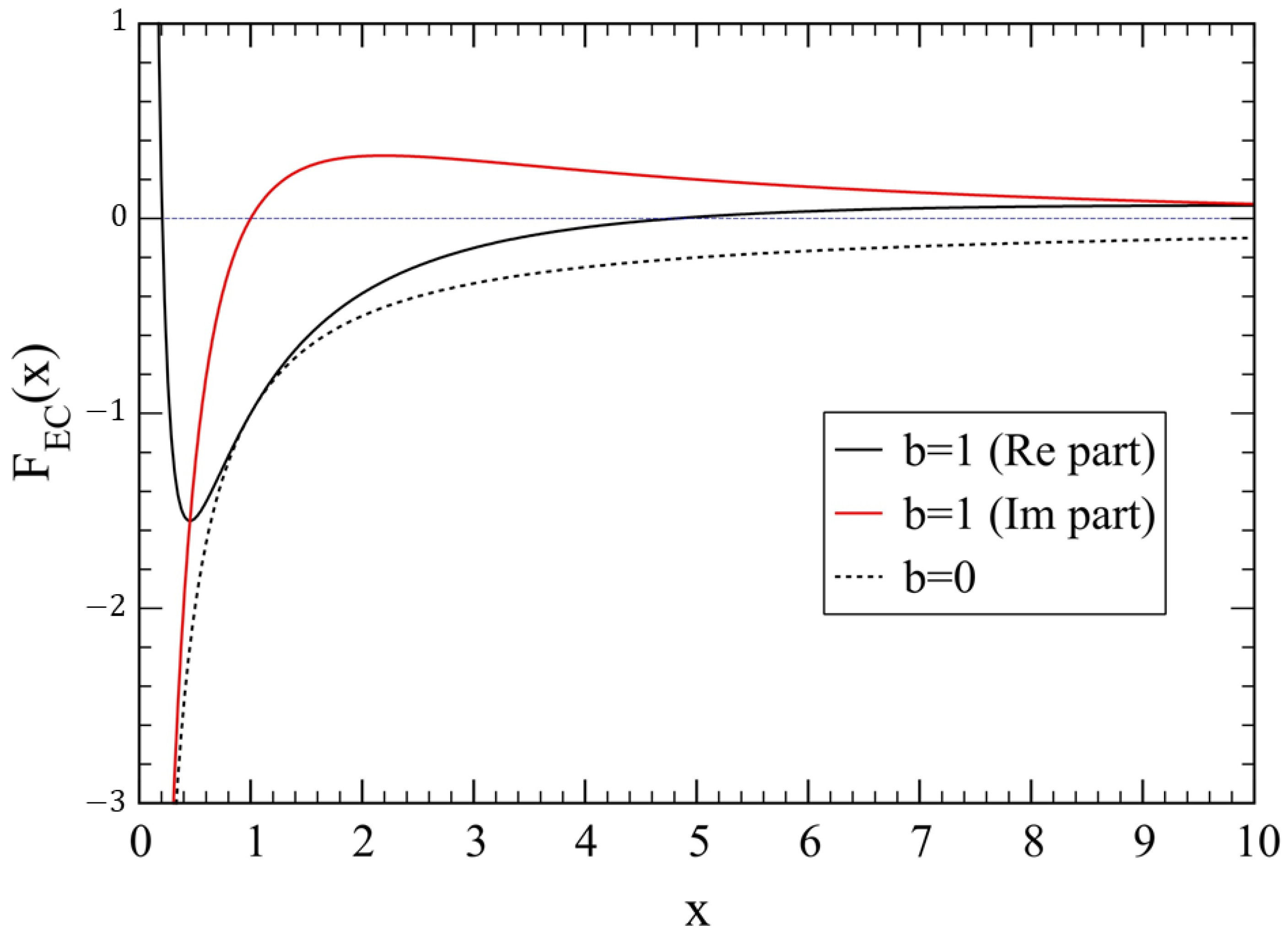
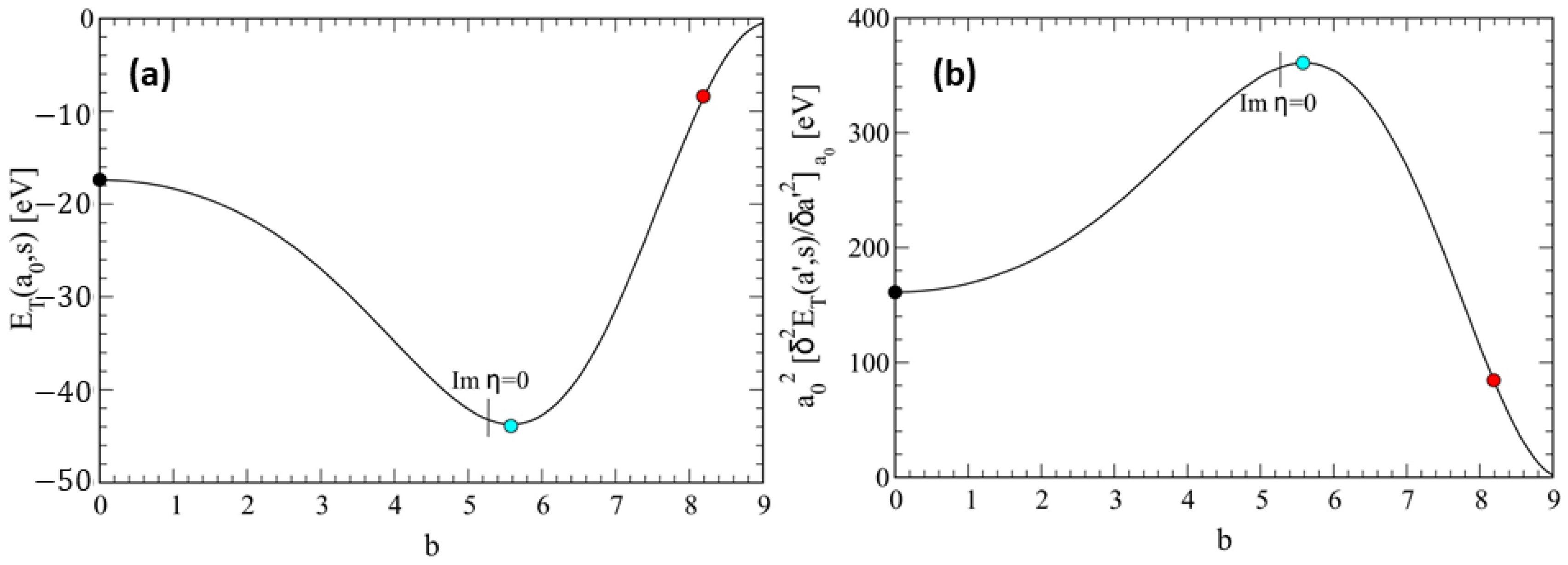
3.2. ERD Complex Lattices: Beyond the Standard Picture

In real systems, there are interactions beyond the Coulomb force. Specifically, the repulsive short-range interaction, given by Equation (10), arises from a non-trivial combination of both electrostatic and quantum mechanical effects, such as those due to the Pauli exclusion principle. These short-range interactions are challenging to calculate, but significant progress has been made by employing density functional theory for the electron states, coupled with molecular dynamics for the ions [25].
For medium-range distances, the van der Waals (VDW) interaction can play an important role, particularly between neutral closed-shell atoms. It can be understood as an induced attractive dipole–dipole interaction (see [19] for a simple derivation of its origin). In the case of ions, the VDW interaction also contributes to the total energy, introducing specific power-law terms that decay with the typical sixth-power exponent. These additional terms can be analyzed in the same way as the Coulomb interaction, leading to a lattice sum (see, e.g., [16]). A review of different types of lattice sums is provided in [26].
There are also phenomena related to vacuum polarization and self-energy effects on electrons, which are generally expected to be quite small. However, much less is known about these effects in confined systems, such as molecules or chains of atoms. Last but not least, electrons can interact with each other through the vibrational modes of the lattice, known as phonons, which play a crucial role in superconductivity (see, e.g., the book on finite fermionic systems that discusses these issues in detail [27]).
In order to take into account these complex scenarios in a simple way, we suggest to introduce an effective Coulomb (EC) interaction between charges separated by a distance r, of the form (Conjecture Equation (1), with a = 1 ),
V EC ( x ) = ± V 0 1 x s , with s = 1 + i b ,
where x = r / a 0 , and, for convenience, we define V EC ( x ) = V 0 F EC ( x ) , with V 0 > 0 , where
F EC ( x ) = ± 1 x cos ( b log x ) i sin ( b log x ) ,
is a complex scaling function. The latter is illustrated in Figure 3 for opposite charges (i.e., corresponding to the negative sign in Equation (15)), and few values of b, for x min < x < 2 . The lower limit is arbitrary (we use x min = 0.1 in the plot), and it has been introduced in order to avoid the non-physical oscillations of F EC ( x ) when x 0 .
It is interesting to note that, due to the cosine function, the real part of the scaling function becomes less attractive and even repulsive, compared to the bare Coulomb decay, 1 / x , suggesting some form of screening effect between charges. A plot for the case b = 1 is shown in Figure 4 over a longer range, 0.1 < x < 10 .
In the following, we apply this model to the ionic lattice and examine its effects on the total lattice energy and the stability criteria of the chain. To this end, we rewrite Equation (8) so that it is of the form
E 0 j EC ( s ) = q I 2 4 π ϵ 0 1 a 0 ( 1 ) j 1 ( | x j | / a 0 ) s , | j | 1 , s = 1 + i b ,
in which we retain the presence of alternating charges, q I = ± q b e , where q b is still a positive real number obeying q 0 = q . Therefore, denoting E EC ( n , s ) E 0 j EC ( s ) , Equation (17) becomes,
E EC ( n , s ) = α 0 q b 2 c a 0 ( 1 ) n 1 n s , n 1 ,
such that Equations (17) and (18) reduce to Equations (8) and (9) when b = 0 . To keep the model as simple as possible, we retain the Born exponential form for the repulsive interaction, as in Equation (10), so that the total lattice energy per site, E T ( a , s ) , can be written as
E T ( a , s ) = 2 E 0 e a / ρ 2 α 0 q b 2 c a η ( s ) , s = 1 + i b .
Due to the presence of η ( s ) , this model brings us close to the issue of non-Hermiticity mentioned in the introduction. Further analytical work would be required to implement the effective Coulomb model for applications in quantum systems [10,11,12]. Since we are dealing with a complex expression for the total energy, Equation (19), we stipulate that the physical value is given by [ E T ( a , s ) ] , which corresponds to taking [ η ( s ) ] in (19).
The stability conditions are then the same as those obtained in Equations (12) and (13), with η ( 1 ) replaced by [ η ( s ) ] and q by q b , where now a 0 ( b ) is a function of b. The final expression for the total energy is then given by (Equation (2) with s = 1 + i b )
E T ( a 0 , s ) = 2 α 0 q b 2 [ η ( 1 + i b ) ] c a 0 ( b ) 1 ρ a 0 ( b ) .
To illustrate the behavior of the total lattice energy in the presence of a complex Coulomb exponent, s = 1 + i b , we have plotted the real values of E T ( a , s ) in Figure 5a, using Equation (19). The values of b chosen for the figure correspond to b = 0 as the reference case, b 5.58 , yielded the lowest possible lattice energy per site and a case with a larger value of E T ( a , s ) , namely b 8.19 .
In Figure 5b, we display the lattice constant, a 0 ( b ) , as a function of b, showing that the most stable situation occurs for b 5.58 , where a 0 0.93425 , being about 10% smaller than in the standard case, b = 0 . For b > 5.58 , the energy increases, and so does the lattice constant. This behavior is related to the fact that η ( 1 + i b ) = 0 when b = 2 π / log 2 9.065 , as discussed in Equation (7). Clearly, since the generalized Coulomb term vanishes, the lattice becomes unstable, and no bound state can exist.
It is interesting to observe that the vanishing of [ η ( 1 + i b 1 ) ] occurs at b 1 5.27185 (see the position of the vertical line in Figure 5b), which is close to b 0 5.58 , where the minimum of the total lattice energy occurs. This difference can be easily eliminated by adjusting the parameters of the model. For example, we fit the ‘renormalized’ charge, q b 1 , so that the minimum of a 0 occurs at b 1 5.27185 where [ η ( 1 + i b 1 ) ] = 0 . This is achieved by imposing the condition, q b 1 2 [ η ( 1 + i b 1 ) ] = [ η ( 1 + i b 0 ) ] , yielding,
q b 1 = [ η ( 1 + i b 0 ) ] / [ η ( 1 + i b 1 ) ] 1.0056 1 ,
which is remarkably close to q = 1 .
In Figure 6a, we show the results for E T ( a 0 , s ) as a function of b, which are consistent with the previous ones. In Figure 6b, we consider the lattice ‘stiffness’, represented by the second derivative of the energy with respect to the lattice constant, as given in Equation (13), with η ( 1 ) replaced by [ η ( s ) ] , and q b = 1 . The phenomenon of stiffness may also have consequences for the electron–phonon couplings, possibly leading to enhanced effective electron–electron exchange, which is important for the emergence of superconductivity properties in materials (see e.g., [28]). We can argue that finite values of the imaginary component b > 0 may result from the interaction of matter waves with vacuum energy fluctuations, thus having a purely quantum nature. Therefore, the small excess charge appearing in Equation (21) can be interpreted as being supplied by the vacuum.

4. The ERD Complex Lattices Within the Range: 1 / 2 a 2

In the following, we consider the general case s = a + i b in the expression of the total lattice energy per site (cf. Equation (20)),
E T ( a 0 , s ) = 2 α 0 q b 2 [ η ( a + i b ) ] c a 0 ( b ) 1 ρ a 0 ( b ) ,
to complement the results discussed in Section 3.2. We do not attempt to relate the ERD lattice model to the question of the non-trivial zeros of η ( s ) . Instead, we study Equation (22) in the range 1 / 2 a 2 , which includes the critical strip 0 < a < 1 . Some illustrative results are reported in Figure 7.
In Figure 7a, we show the behavior of the equilibrium lattice constant, a 0 ( s ) , s = a + i b , as a function of a for selected values of b. We observe that a 0 ( s ) decreases with increasing a, as expected, but for b 3 , the opposite trend occurs, with a 0 ( s ) increasing with a. This suggests that the physics may depend crucially on the imaginary component, b. Similar results are shown in Figure 7b, where a 0 ( s ) is plotted versus b for some values of a, showing a crossover of the curves near b c 3.2 . In this case, the values a 0 ( 1 / 2 , b ) are the largest for b < b c and the smallest for b > b c . Thus, for the latter, the case a = 1 / 2 is more stable than for larger values of a.
The results for the total lattice energy per site, E T ( a 0 , s ) (Figure 7c), and for the lattice stiffness (Figure 7d), plotted as a function of b, are consistent with those shown in Figure 7b. These results suggest a quite rich scenario of the physics of strongly interacting systems modeled by the simple ERD lattice, which deserves further consideration, both theoretically and experimentally.
For the interested reader, we have also prepared two appendices dealing with the Riemann hypothesis: The first, in Appendix B, reviews the connection between ζ ( s ) and prime numbers, which contains a wealth of numerical results that complement those in the literature [29,30,31,32,33,34,35,36,37]. The second, in Appendix C, discusses simple arguments related to the Riemann hypothesis.

5. Concluding Remarks

We have presented an application of the Dirichlet η ( s ) function to describe 1D ionic systems with alternating charges characterized by a complex Coulomb exponent s = 1 + i b . This leads to an effective interaction, V EC ( r ) ± q 2 / r s , between charges ± q separated by a distance r, where the case b = 0 corresponds to the standard Coulomb law. The effects of a finite imaginary component, b > 0 , were studied by calculating the cohesive energy of a 1D lattice, E T ( a 0 , b ) [ η ( s ) ] , from which a new lattice constant, a 0 ( b ) , is obtained as a function of b. For small values of b, the lattice shrinks, i.e., a 0 ( b ) < a 0 ( 0 ) , and its cohesive energy decreases, E T ( a 0 , b ) < E T ( a 0 , 0 ) . Both the lattice constant and the cohesive energy reach a minimum at b 5.58 and then start increasing again for larger values of b. Correspondingly, the lattice stiffness, represented by the second derivative 2 E T / a 2 | a 0 , reaches a maximum at b 5.58 and begins to decrease for b > 5.58 . Finally, the lattice becomes unstable when η ( 1 + i b u ) = 0 , with b u = 2 π / log 2 9.065 .
We argue that the imaginary component b > 0 could result from effective many-body interactions between localized electrons due to their coupling with phonons and vacuum energy fluctuations. Further theoretical work is needed to quantitatively validate these ideas by comparing the model with experimental observations in various physical contexts. Specifically, applications to real three-dimensional structures require the use of generalized forms of the η ( s ) function to deal with more elaborated lattice sums (see, e.g., [16,26]).
Finally, the connection between the Riemann zeta function and prime numbers has also been explored in light of the ongoing interest in the still unproven Riemann hypothesis. Numerical calculations on the prime numbers gaps distribution, as well as an evaluation of their correlations using a fluctuation analysis method, are discussed. The former follows an exponentially decaying distribution function, which is derived numerically from the first two million primes. The fluctuation analysis reveals that hidden correlations exist between gaps, which tend to disappear as the number of primes increases. This gradual approach to the asymptotic behavior is typical of other quantities, such as the prime number value as a function of the number of primes considered. Finally, we demonstrate that the non-trivial zeros of the Riemann zeta function, ρ = a + i b , exhibit distinct behaviors depending on whether the real part satisfies a = 1 / 2 or a 1 / 2 . This difference is significant and may suggest that actual zeros can exist only when a = 1 / 2 .

Funding

This research received no external funding.

Data Availability Statement

Data used for the calculations will be made available on request.

Acknowledgments

I have beneffited from discussions with F. Alasia, G. Benedek, R.A. Broglia, G. Colò, G. Onida, Ll. Serra, and M.P. Tosi. I dedicate this review to the memory of Mario P. Tosi (1932–2015) [38].

Conflicts of Interest

The author declares no conflict of interest.

Appendix A. The Dirichlet Function η(s)

Let us briefly review the derivation of Equation (6) in the case ( s ) > 1 where ζ ( s ) is convergent. To do this, we consider the partial sums, η 2 m ( s ) = n = 1 2 m ( 1 ) n 1 n s , with integer m > 0 , so that
(A1) η 2 m ( s ) = 1 1 2 s + 1 3 s 1 4 s + ( 1 ) 2 m ( 2 m ) s , (A2) = 1 + 1 2 s + 1 3 s + 1 4 s + 1 ( 2 m ) s 2 1 2 s + 1 4 s + 1 6 s + 1 ( 2 m ) s , (A3) = ζ 2 m ( s ) 2 1 s 1 + 1 2 s + 1 3 s + 1 4 s + 1 m s , (A4) = ( 1 2 1 s ) ζ 2 m ( s ) + 2 1 s n = m + 1 2 m 1 n s ,
where the summation in the second term can be written as
n = m + 1 2 m 1 n s = 1 m s 1 ( 1 + 1 / m ) 2 + 1 ( 1 + 2 / m ) 2 + + 1 ( 1 + m / m ) s < m 1 s ,
which vanishes when m since, by assumption, ( s ) > 1 . In this limit, both partial sums, η 2 m ( s ) and ζ 2 m ( s ) , tend to their full series, η ( s ) and ζ ( s ) , respectively, yielding Equation (6). Now, if we use the latter in Equation (4), we find the functional form obeyed by η ( s ) (see also [23]), that is,
1 π s / 2 Γ s 2 η ( s ) 1 2 1 s = 1 π ( 1 s ) / 2 Γ 1 s 2 η ( 1 s ) 1 2 s .
In particular, for s 0 one has Γ ( s / 2 ) 2 / s , Γ ( 1 / 2 ) = π , and using the Taylor expansion for log ( 1 + x ) with | x | < 1 , together with Abel’s theorem, allows one to prove that indeed η ( 1 ) = log 2 , yielding η ( 0 ) = 1 / 2 .

Appendix B. Some Properties of Prime Numbers and the Riemann Hypothesis

There is an explicit connection between ζ ( s ) and the prime numbers, denoted as the Euler product formula (proved by Euler for real s), which can be written using the logarithm as follows,
log ζ ( s ) = i = 1 log 1 1 [ P ( i ) ] s , s = a + i b ,
where the sum runs over all prime numbers, P ( 1 ) = 2 , P ( 2 ) = 3 , etc., which was used by Riemann to introduce the complex function carrying his name [21]. He also found an empirical relation between the function π ( x ) , which counts the number of primes not exceeding the value x, and Li ( x ) = 2 x d t / log t , denoted as the logarithmic integral.
The prime number theorem (PNT) asserts that π ( x ) x / log x , for x , and it was proved by Hadamard in 1896. Finally, with the use of Riemann’s work, the best possible approximation to π ( x ) can be achieved in the form [29],
π ( x ) = R ( x ) n = 1 R ( x ρ n ) , with R ( x ) = Li ( x ) n = 2 1 n Li ( x 1 / n ) ,
where ρ n = 1 / 2 + i b n are the non-trivial zeros of ζ ( s ) , with b n ± (14.134, 21.022, 25.010, ...) [30]. The fact that a = 1 / 2 constitutes the Riemann hypothesis means that there are no non-trivial zeros within the critical strip, 0 < a < 1 , other than on the critical line at a = 1 / 2 .

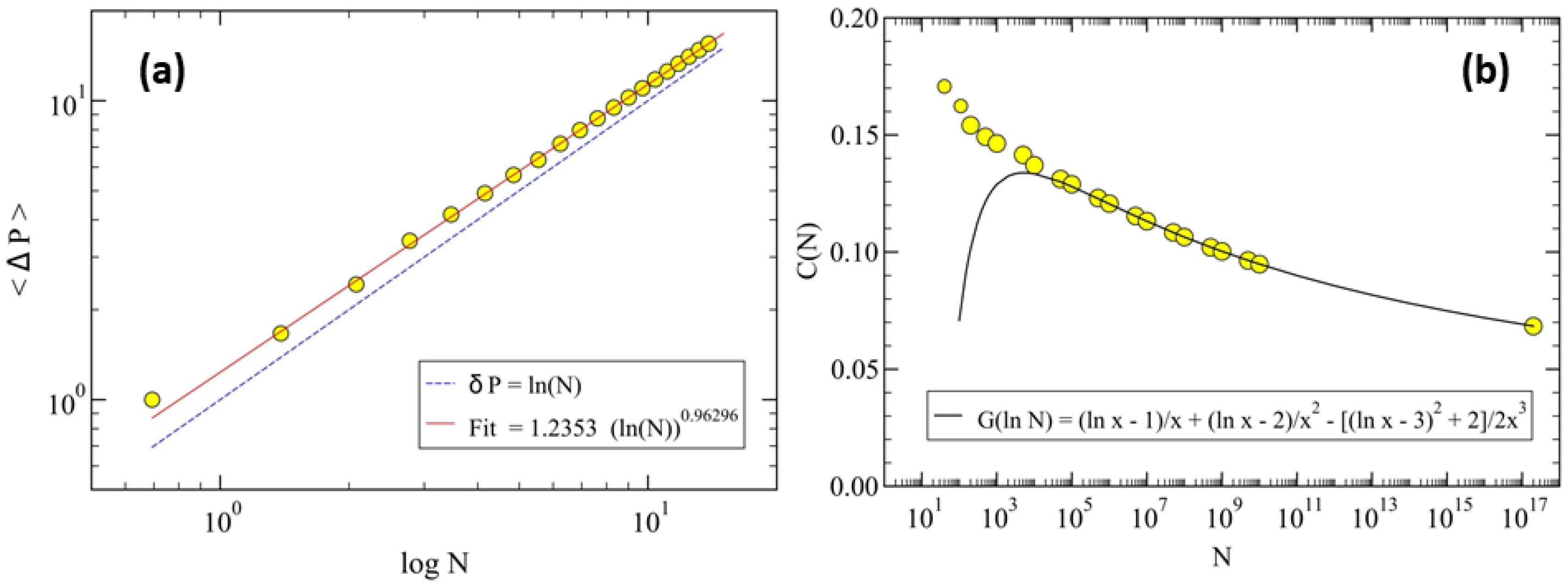
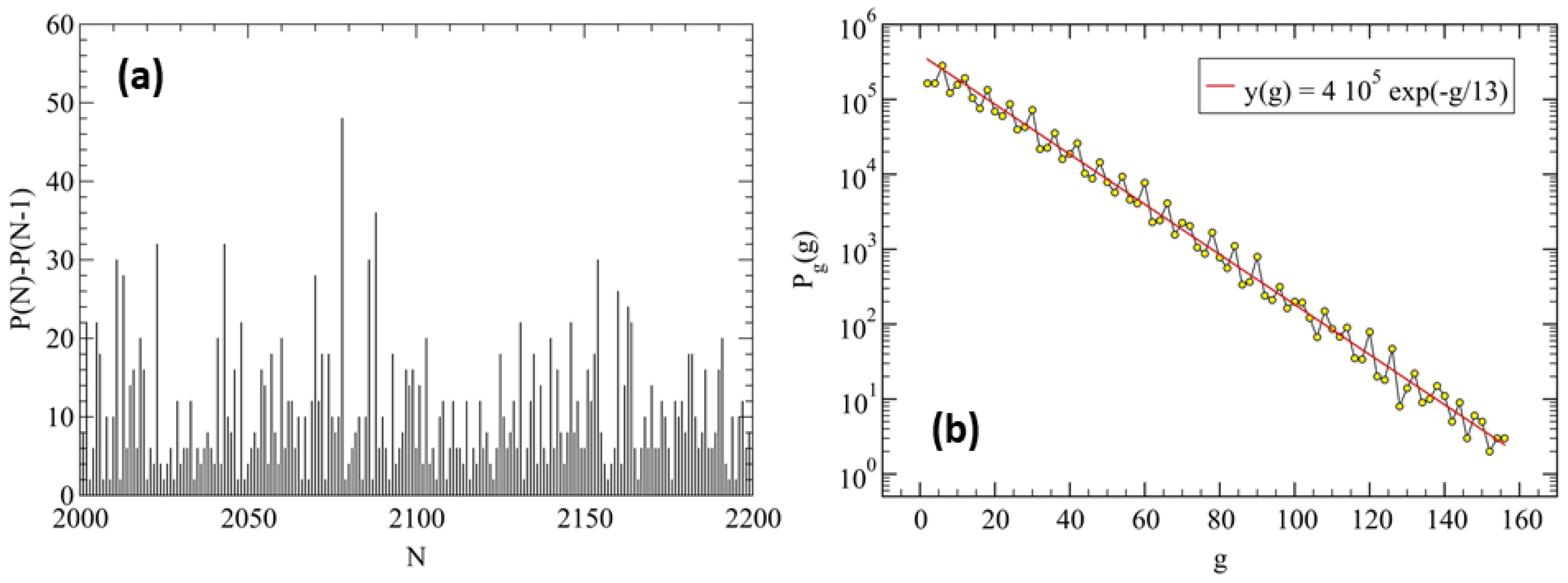
Appendix B.1. Numerical Results on Prime Numbers

In the following, we study the properties of prime numbers related to the PNT. It can be shown that if PNT holds, then the Nth prime number, P ( N ) N log N [31]. We perform a numerical analysis on P ( N ) by first looking at the mean distance between sequential primes, P ( N ) P ( N 1 ) , as a function of N, as shown in Figure A1a. It can be shown that the mean sequential distance obeys, Δ P ( N ) = ( P ( N ) P ( 1 ) ) / N log N , in accordance with the numerical results. To be noted, though, is that the asymptotic logarithmic dependence is approached very slowly. To illustrate this behavior, we have fitted the numerical results with an effective power-law, ( log N ) α , yielding α 0.96296 up to N = 10 6 (red line in the figure).
Figure A1. (a) The mean distance, Δ P , between sequential prime numbers, P ( N ) P ( N 1 ) , as a function of the logarithm of N, for 2 N 10 6 , i.e., 0.693 log N 13.82 . For comparison, we have added the linear dependence, Δ P ( N ) log N (dashed line), suggesting that P ( N ) N log N , asymptotically. The continuous red line is a fit to the data, excluding the first point at ( log 2 ,1), yielding F = 1.2353 ( log N ) 0.96296 . (b) The function C ( N ) = P ( N ) / ( N log N ) 1 (yellow circles), together with the approximation (black line): G ( x ) = ( log x 1 ) / x + ( log x 2 ) / x 2 [ ( log x 3 ) 2 + 2 ] / ( 2 x 3 ) , where x = log N [32]. The point at N = 2 10 17 corresponds to the prime 8512677386048191063, i.e., P ( N ) 8.513 10 18 , yielding C ( N ) 0.0684765 . The selected values of P ( N ) up to N 10 10 were obtained from the Web.
Mathematics 13 00570 g0a1
In Figure A1b, we show the deviations of P ( N ) from its asymptotic behavior in terms of a correction factor C ( N ) , such that P ( N ) = [ 1 + C ( N ) ] N log N , defined according to
C ( N ) = P ( N ) N log N 1 ,
which should behave as C ( N ) 0 when N . The continuous line shown in the figure is an approximation to C ( N ) due to Cesàro [32] valid for N > 10 4 (see also [33,34]).
It is also interesting to study the distribution of ‘gaps’ between consecutive primes defined as, g = P ( N ) P ( N 1 ) , with N 2 . An example of a series of gaps is shown in Figure A2b. A related quest regards the estimation of the largest gap within the first N prime numbers. It is suggested that such maximal gaps occur for primes, P ( g ) exp ( c g ) , with c 1 [35] (see also [36] for large gaps).
Figure A2. (a) A typical profile of sequential prime numbers gaps, P ( N ) P ( N 1 ) , vs. N. We note that the maximal gap shown here, g = 48 at N = 2078 corresponding to P ( N ) 18,100, is consistent with the conjecture, log P ( N ) c g , with c 1.415 , and c ( g ) 1 when g [35]. (b) Distribution of gaps, P g ( g ) , vs. g. The red line is a guide to the eyes displaying the exponential decay, y ( g ) = 4 × 10 5 exp ( g / 13 ) .
Mathematics 13 00570 g0a2
As one can see from Figure A2a, the sequence of gaps looks random, and in order to characterize them, we first calculate their distribution function. As shown in Figure A2b, the latter appears to be consistent with a simple exponential decay, with a characteristic mean gap, g 13 , at least within the first two million primes considered. The question arises as to whether the gaps may still display some kind of auto-correlations.

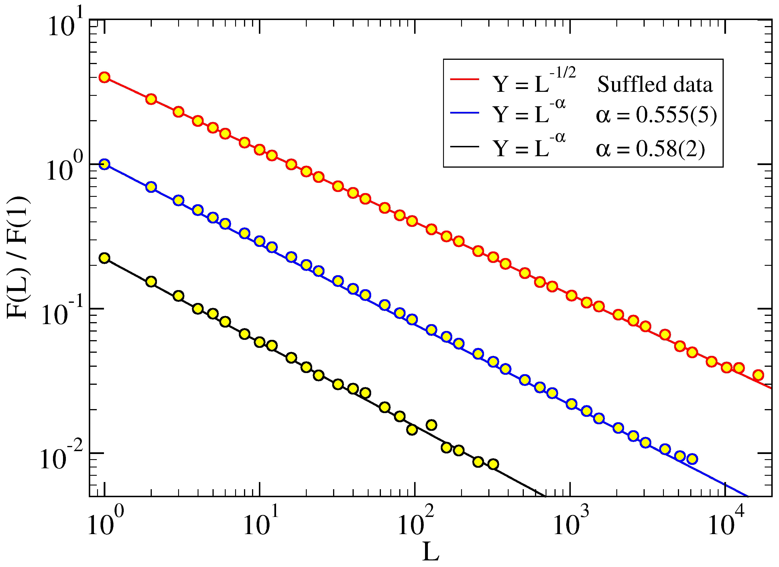
Appendix B.2. Fluctuation Analysis

To see this, we apply the so-called fluctuation analysis, which allows us to detect auto-correlations if they are present in a random series [37]. We briefly discuss the method adapted to a series of gaps like the one shown in Figure A2a. Let us denote by L 0 the total length of the series, for instance L 0 = 200 in the figure. Next, we divide the total length into M boxes of length L, such that, M L = L 0 . Within each box j, we calculate the average value, B j ( L ) , defined as
B j ( L ) = 1 L i = 1 L R ( j L L + i ) , 1 j M ,
where R ( n ) denotes the amplitude of the series at location n, with 1 n L 0 .
Then, we evaluate the mean fluctuations, F 2 ( L ) , of the B j ( L ) at ‘length scale’ L, yielding,
F 2 ( L ) = 1 M j = 1 M 1 B j + 1 B j ( L ) 2 2 B 2 B 2 .
In the following, we consider the case of uncorrelated random numbers, R n , drawn from an exponential distribution function, P ( R ) = R 0 1 exp ( R / R 0 ) . This is similar to P g ( g ) for the gaps between primes, and for simplicity, it is assumed to be normalized according to 0 d r P ( r ) = 1 .
For this simple model we can obtain analytical results for the first two moments of the distribution, i.e.,
(A12) B ( L ) = R = R 0 , (A13) B 2 ( L ) = 1 L 2 L R 2 + 1 2 L ( L 1 ) R 2 = 1 L 2 L 2 R 0 2 + 1 2 L ( L 1 ) R 0 2 ,
yielding the following result for F 2 ( L ) ,
F 2 ( L ) = 4 L R 0 2 1 + 1 4 L 1 L ,
which can be written in the more convenient form as follows,
F ( L ) F ( 1 ) = 1 + 1 4 L 1 L 1 / 2 L 1 / 2 .
The numerical results for the prime gaps are shown in Figure A3, where we have fitted effective power-laws, F ( L ) L α ( N ) , yielding the exponent α ( N ) , in order to detect possible departures from the uncorrelated case, Equation (A15). Indeed, we find deviations from the exponent 1/2 at small L, where α ( N ) decreases from α ( N ) 0.58 ( 2 ) , for N = 10 5 prime numbers, down to α ( N ) 0.555 ( 5 ) , for N = 10 6 .
The case of shuffling the prime gaps, shown as the red circles in the figure, indeed displays the uncorrelated behavior with α = 1 / 2 . We may conclude that the observed departures of F ( L ) from the uncorrelated regime depend on the number of primes N considered, such that α ( N ) 1 / 2 when N . The asymptotic behavior is approached very slowly, similarly to the other quantities discussed previously, e.g., P ( N ) as described by Equation (A9).
Figure A3. Fluctuation analysis of distances profiles: F ( L ) / F ( 1 ) vs. L. The numercial data are fitted with the power law, F ( L ) L α , for the cases N = 10 5 (dark-yellow circles), where the straight line has slope α = 0.58 ( 2 ) ; N = 2 × 10 6 (blue-white circles), with α = 0.555 ( 5 ) ; N = 2 × 10 6 (red-white circles), suffled data yielding α = 1 / 2 . The data have been shifted for visual convenience.
Mathematics 13 00570 g0a3

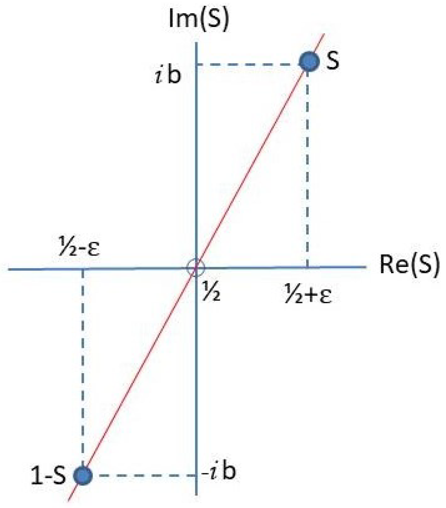
Appendix C. The Non-Trivial Zeros of ζ(s) Within: 0 < a < 1

In order to elaborate on the locations of possible zeros of ζ ( s ) , s = a + i b , within the critical strip 0 < a < 1 , let us write Equation (4) in the form reported in Equation (A6),
1 π s / 2 Γ s 2 ζ ( s ) = 1 π ( 1 s ) / 2 Γ 1 s 2 ζ ( 1 s ) .

Appendix C.1. The Case a = 1/2

Motivated by the (not yet proved) Riemann hypothesis [21] that the non-trivial zeros of ζ ( s ) occur only for a = 1 / 2 , we consider next the case, s = 1 / 2 + i b , and, 1 s = 1 / 2 i b , so that Equation (A16) becomes,
A ( b ) 1 π i b / 2 Γ 1 4 + i b 2 ζ 1 2 + i b = 1 π i b / 2 Γ 1 4 i b 2 ζ 1 2 i b A * ( b ) ,
yielding, A ( b ) = A * ( b ) , implying that ( A ( b ) ) = 0 , i.e., A ( b ) is a real-valued function of b. To proceed further, we denote the real and imaginary components of the functions building A ( b ) as follows,
π i b / 2 = Π R ( b ) + i Π I ( b ) ,
where Π R = cos [ ( b / 2 ) log π ] , and Π I = sin [ ( b / 2 ) log π ] , i.e., Π R 2 + Π I 2 = 1 . For Γ ( s / 2 ) , we define,
Γ 1 4 + i b 2 = Γ R ( b ) + i Γ I ( b ) ,
and for the Riemann zeta function,
ζ 1 2 + i b = ζ R ( b ) + i ζ I ( b ) .
Next, using Equations (A18)–(A20), the auxiliary function A ( b ) can be written as
A ( b ) = ( Π R + i Π I ) ( Γ R + i Γ I ) ( ζ R + i ζ I ) = A R ( b ) + i A I ( b ) ,
where
(A22) A R ( b ) = ζ R Π R Γ R Π I Γ I ζ I Π R Γ I + Π I Γ R , (A23) A I ( b ) = ζ R Π R Γ I + Π I Γ R + ζ I Π R Γ R Π I Γ I .
Now, the condition found above for A ( b ) yields A I ( b ) = 0 , from which we can find a relation between the components ζ R and ζ I according to
ζ R ( b ) = ζ I ( b ) Π R Γ R Π I Γ I Π R Γ I + Π I Γ R = ζ I ( b ) Γ R cos ( α ) + Γ I sin ( α ) Γ I cos ( α ) Γ R sin ( α ) ,
where α = ( b / 2 ) log π , suggesting that the following result holds:
ζ R ( b ) F R = ζ I ( b ) F I = ζ 0 ( b ) ,
where ζ 0 ( b ) , F R = Γ R cos ( α ) + Γ I sin ( α ) , and F I = Γ I cos ( α ) Γ R sin ( α ) , obeying the relation F R 2 + F I 2 = Γ R 2 + Γ I 2 = | Γ ( 1 / 4 + i b / 2 ) | 2 . Using Equation (A25), we can write ζ 0 ( b ) in terms of ζ ( 1 / 2 + i b ) as follows,
ζ 0 ( b ) = ζ ( s ) Γ ( s / 2 ) | Γ ( s / 2 ) | 2 e i α , s = 1 2 + i b .
where the product ζ 0 ( b ) | Γ ( s / 2 ) | is known as the Hardy function [22,30].

Appendix C.2. The General Case 0 < a < 1

Let us next consider the general case, s = a + i b , with a = 1 / 2 + ε , and 0 ε < 1 / 2 . Now, Equation (A16) yields, with β = ε + i b ,
π β / 2 Γ 1 4 + β 2 ζ 1 2 + β = π β / 2 Γ 1 4 β 2 ζ 1 2 β ,
thus connecting values of ζ ( s ) for s = 1 / 2 + β and 1 s = 1 / 2 β (see Figure A4).
Figure A4. The two points in the complex plane, s = 1 / 2 + ε + i b and 1 s = 1 / 2 ε i b , are connected via the functional form in Equation (A27). The red straight line is a guide for the eyes. A second pair of solutions corresponds to s = 1 / 2 ε + i b and 1 s = 1 / 2 + ε i b .
Mathematics 13 00570 g0a4
We can write the L.H.S. of Equation (A27) in the same form as in Equations (A22) and (A23) evaluated at s = 1 / 2 + β , while the R.H.S. of Equation (A27) is written in terms of A R ( 1 s ) and A I ( 1 s ) , as follows,
(A28) A R ( s ) = ζ R ( s ) B RR ( s ) ζ I ( s ) B IR ( s ) = A R ( 1 s ) , (A29) A I ( s ) = ζ R ( s ) B RI ( s ) + ζ I ( s ) B II ( s ) = A I ( 1 s ) ,
where B RR = B II = Π R Γ R Π I Γ I , B IR = B RI = Π R Γ I + Π I Γ R . The solution can be written as a function of A R , I ( 1 s ) , yielding,
(A30) ζ R ( s ) = B RR ( s ) A R ( 1 s ) + B IR ( s ) A I ( 1 s ) / D ( s ) , (A31) ζ I ( s ) = B RI ( s ) A R ( 1 s ) + B RR ( s ) A I ( 1 s ) / D ( s ) ,
where the determinant of the coefficients, D ( s ) , becomes,
D ( s ) = B RR 2 ( s ) + B RI 2 ( s ) = π ε Γ R 2 + Γ I 2 = π ε | Γ ( s / 2 ) | 2 > 0 .
For illustration, we can apply Equations (A30)–(A32) to the previous case, ε = 0 . For the latter, we found that A I ( s ) = A I ( 1 s ) = 0 , yielding,
(A33) ζ R ( s ) = B RR ( s ) A R ( 1 s ) 1 D ( s ) , (A34) ζ I ( s ) = B RI ( s ) A R ( 1 s ) 1 D ( s ) ,
which is equivalent to Equation (A25) with,
ζ 0 ( s ) = A R ( 1 s ) 1 D ( s ) = A R ( s ) 1 D ( s ) .
As an attempt to shed light on the question of whether ζ ( s ) may have zeros for a 1 / 2 , we investigate the conditions that Equations (A30) and (A31) must satisfy in order to behave as in Equations (A25), (A33) and (A34), when a = 1 / 2 , yielding a linear relationship between ζ ( s ) and a real function ζ 0 ( s ) (Equation (A26)).
To this end, let us write Equations (A30) and (A31) as follows,
(A36) ζ R ( s ) = B RR ( s ) A R ( 1 s ) 1 D ( s ) 1 + B RI ( s ) B RR ( s ) A I ( 1 s ) A R ( 1 s ) , (A37) ζ I ( s ) = B RI ( s ) A R ( 1 s ) 1 D ( s ) 1 B RR ( s ) B RI ( s ) A I ( 1 s ) A R ( 1 s ) .
Next, if the two factors within parenthesis in the R.H.S. of (A36) and (A37) obey,
1 + B RI ( s ) B RR ( s ) A I ( 1 s ) A R ( 1 s ) = ζ ˜ R ( s ) , 1 B RR ( s ) B RI ( s ) A I ( 1 s ) A R ( 1 s ) = ζ ˜ I ( s ) ,
with ζ ˜ R ( s ) = ζ ˜ I ( s ) , then ζ ( s ) can be represented by a single real function, as in Equation (A26). This can only happen if,
B RI B RR = B RR B RI B RR 2 + B RI 2 = D ( s ) = 0 .
This result implies that the condition for a real-valued function ζ 0 ( s ) , whose zeros should determine those of ζ ( s ) for ε > 0 , holds only when D ( s ) = 0 . However, this contradicts Equation (A32), where D ( s ) > 0 . We can therefore conclude that no solution ζ ( s ) = 0 exists based on a relation similar to that in Equation (A26) for the case ε > 0 .

References

  1. Schumayer, D.; Hutchinson, D.A. Colloquium: Physics of the Riemann Hypothesis. Rev. Mod. Phys. 2011, 83, 307–330. [Google Scholar] [CrossRef]
  2. Remmen, G.N. Amplitudes and the Riemann zeta function. Phys. Rev. Lett. 2021, 127, 241602. [Google Scholar] [CrossRef] [PubMed]
  3. Wolf, M. Will a physicist prove the Riemann hypothesis? Rep. Prog. Phys. 2020, 83, 036001. [Google Scholar] [CrossRef] [PubMed]
  4. Barbarani, V. A Quantum Model of the Distribution of Prime Numbers and the Riemann hypothesis. Int. J. Theor. Phys. 2020, 59, 2425–2470. [Google Scholar] [CrossRef]
  5. Tamburini, F.; Licata, I. Majorana quanta, string scattering, curved spacetimes and the Riemann Hypothesis. Phys. Scr. 2021, 96, 125276. [Google Scholar] [CrossRef]
  6. Abdelaziz, S.; Shaker, A.; Salah, M.M. Development of a New Zeta Formula and Its Role in Riemann Hypothesis and Quantum Physics. Mathematics 2023, 11, 3025. [Google Scholar] [CrossRef]
  7. Tschaffon, M.E.N.; Tkáčová, I.; Maier, H.; Schleich, W.P. A Primer on the Riemann Hypothesis. In Sketches of Physics; Citro, R., Lewenstein, M., Rubio, A., Schleich, W.P., Wells, J.D., Zank, G.P., Eds.; Lecture Notes in Physics 1000; Springer: Cham, Switzerland, 2023; Chapter 7. [Google Scholar] [CrossRef]
  8. Schuch, D.; Chung, K.M.; Hartmann, H. Nonlinear Schrödinger-type field equation for the description of dissipative systems. I. Derivation of the nonlinear field equation and one-dimensional example. J. Math. Phys. 1983, 24, 1652–1660. [Google Scholar] [CrossRef]
  9. Bulyzhenkov, I.E. Complex charge densities unify particles with fields and gravitation with electricity. Bull. Lebedev Phys. Inst. 2016, 43, 138–142. [Google Scholar] [CrossRef]
  10. Ashida, Y.; Gong, Z.; Ueda, M. Non-Hermitian Physics. Adv. Phys. 2020, 69, 249–435. [Google Scholar] [CrossRef]
  11. Bender, C.M. Making sense of non-Hermitian Hamiltonians. Rep. Prog. Phys. 2007, 70, 947. [Google Scholar] [CrossRef]
  12. Matsoukas-Roubeas, A.S.; Roccati, F.; Cornelius, J.; Xu, Z.; Chenu, A.; del Campo, A. Non-Hermitian Hamiltonian deformations in quantum mechanics. J. High Energy Phys. 2023, 2023, 1–31. [Google Scholar] [CrossRef]
  13. LeClair, A. Riemann hypothesis and random walks: The zeta case. Symmetry 2021, 13, 2014. [Google Scholar] [CrossRef]
  14. Orús-Lacort, M.; Orús, R.; Jouis, C. Analyzing Riemann’s hypothesis. Ann. Math. Phys. 2023, 6, 75–82. [Google Scholar] [CrossRef]
  15. Silva, S.D. The Riemann Hypothesis: A Fresh and Experimental Exploration. J. Adv. Math. Comput. Sci. 2024, 39, 100–112. [Google Scholar] [CrossRef]
  16. Tosi, M.P. Cohesion of Ionic Solids in the Born Model. Solid State Phys. 1964, 16, 1–120. [Google Scholar] [CrossRef]
  17. Damm, J.Z.; Chvoj, Z. Optimization of Tosi-Fumi Ionic Radii for F.C.C. Alkali Halide Crystals. Phys. Status Solidi B 1982, 114, 413–418. [Google Scholar] [CrossRef]
  18. Roman, H.E. A Study of Physical Properties of Ionic Systems. Ph.D. Thesis, International School for Advanced Studies (I.S.A.S-S.I.S.S.A), Trieste, Italy, 1983. [Google Scholar] [CrossRef]
  19. Kittel, C. Introduction to Solid State Physics, 8th ed.; John Wiley & Sons, Inc.: Hoboken, NJ, USA, 2005; Available online: https://www.wiley.com/en-us/Introduction+to+Solid+State+Physics%2C+8th+Edition-p-9780471415268 (accessed on 1 January 2025).
  20. Osler, T.J. Euler and the Functional Equation for the Zeta Function. Math. Sci. 2009, 34, 62–73. Available online: https://www.appliedprobability.org/publications/the-mathematical-scientist (accessed on 1 January 2025).
  21. Riemann, B. Ueber die Anzahl der Primzahlen unter einer gegebenen Grösse. Monatsberichte Berl. Akad. VII 1859, 136. Translated by Wilkins, D.R., On the number of prime numbers less than a given quantity. Available online: https://www.claymath.org/wp-content/uploads/2023/04/Wilkins-translation.pdf (accessed on 1 January 2025).
  22. Titchmarsh, E.C. The Theory of the Riemann Zeta Function, 2nd ed.; The Clarendon Press Oxford University Press: Oxford, UK, 1986. [Google Scholar]
  23. Hardy, G.H. Notes on some points in the integral calculus LV: On the integration of Fourier series. Messenger Math. 1922, 51, 186–192, 392. Available online: https://ia800208.us.archive.org/32/items/messengerofmathe5051cambuoft/messengerofmathe5051cambuoft.pdf (accessed on 1 January 2025).
  24. Borwein, P. An Efficient Algorithm for the Riemann Zeta Function. 1995. Available online: https://citeseerx.ist.psu.edu/document?repid=rep1&type=pdf&doi=d9c5d06fadb170ad82f7697c225a610a321d8d0a (accessed on 1 January 2025).
  25. Car, R.; Parrinello, M. Unified Approach for Molecular Dynamics and Density-Functional Theory. Phys. Rev. Lett. 1985, 55, 2471. [Google Scholar] [CrossRef] [PubMed]
  26. Borwein, J.M.; Glasser, M.L.; McPhedran, R.C.; Wan, J.G.; Zucker, I.J. Lattice Sums Then and Now (Encyclopedia of Mathematics and Its Applications No. 150); Cambridge University Press: Cambridge, UK, 2013. [Google Scholar]
  27. Broglia, R.A.; Colò, G.; Onida, G.; Roman, H.E. Solid State Physics of Finite Systems: Metal Clusters, Fullerenes, Atomic Wires, Advanced Texts in Physics; Springer: Berlin, Germany, 2004. [Google Scholar] [CrossRef]
  28. Ziman, J.M. Principles of the Theory of Solids; Cambridge University Press: Cambridge, UK, 1979. [Google Scholar]
  29. Zagier, D. The First 50 Million Prime Numbers. Math. Intell. 1977, 1 (Suppl. S2), 7–19. [Google Scholar] [CrossRef]
  30. Meer, R.V.D. Zeros of the Zeta Function. Ph.D. Thesis, Faculty of Science and Engineering, Mathematics and Applied Mathematics, University of Groningen, Groningen, The Netherlands, 2020. Available online: https://fse.studenttheses.ub.rug.nl/21726/1/bMATH_2020_MeerRvander.pdf (accessed on 1 January 2025).
  31. Apostol, T.M. Introduction to Analytic Number Theory; Springer: New York, NY, USA, 1976. [Google Scholar]
  32. Cesàro, E. Sur une formule empirique de M. Pervouchine. C. R. Math. Acad. Sci. Paris 1894, 119, 848–849. [Google Scholar]
  33. Jakimczuk, R. An approximate formula for prime numbers. Int. J. Contemp. Math. Sci. 2008, 3, 1069–1086. Available online: https://www.m-hikari.com/ijcms-password2008/21-24-2008/jakimczukIJCMS21-24-2008.pdf (accessed on 1 January 2025).
  34. Arias de Reyna, J.; Toulisse, J. The n-th prime asymptotically. J. ThéOrie Nombres Bordx. 2013, 25, 521–555. [Google Scholar] [CrossRef]
  35. Shanks, D. On maximal gaps between successive primes. Math. Comput. 1964, 18, 646–651. [Google Scholar] [CrossRef]
  36. Nicely, T. New maximal prime gaps and first occurrences. Math. Comput. 1999, 68, 1311–1315. [Google Scholar] [CrossRef]
  37. Koscielny-Bunde, E.; Bunde, A.; Havlin, S.; Roman, H.E.; Goldreich, Y.; Schellnhuber, H.J. Indication of a universal persistence law governing atmospheric variability. Phys. Rev. Lett. 1998, 81, 729. [Google Scholar] [CrossRef]
  38. Tosi, M.P. In Memoriam; Department of Physics, University of Trieste: Trieste, Italy, 2015; Available online: https://df.units.it/en/news/14180 (accessed on 1 January 2025).
Figure 1. A one-dimensional ionic crystal: The positive ion (red) located at the center of the chain is taken as the reference for evaluating the total energy of the system. The distance a 0 represents the lattice constant at equilibrium. Typically, negative ions (cyan) are larger than their positive counterparts (red), especially when their atomic numbers are comparable. For example, in KCl, with z K = 19 and z Cl = 17 , the ionic radii are r K + = 1.46 Å and r Cl = 1.58 Å [16,17,18].
Mathematics 13 00570 g001
Figure 2. The total lattice energy per site, E T ( a ) , vs. lattice spacing a , for a one-dimensional ionic crystal. The continuous line represents Equation (11) for the set of parameters: E 0 = 3 × 10 4 eV, ρ = 0.1 × 10 10 m, q = 1 , where we have used c = 0.1974 × 10 6 eV m. The minimum energy, E T ( a 0 ) 17.38 eV (Equation (14)), occurs at a 0 1.039 × 10 10 m (yellow circle). The second derivative, Equation (13), yields, a 0 2 2 E T / a 2 | a 0 161.28 eV.
Mathematics 13 00570 g002
Figure 3. The scaling function F EC ( x ) vs. x (Equation (16)), with s = 1 + i b , and b = ( 2 , 1.5 , 1 , 0.5 , 0 ) . (a) [ F EC ( x ) ] = x 1 cos ( b log x ) . (b) [ F EC ( x ) ] = x 1 sin ( b log x ) . Here, x x min = 0.1 . For x < 1 , the zeros of [ F EC ( x ) ] occur at x k = exp [ π ( 2 k + 1 ) / 2 b ] , with integer k 0 , yielding x 0 ( 0.042 , 0.21 , 0.35 , 0.46 ) for b = ( 0.5 , 1 , 1.5 , 2 ) , respectively. For [ F EC ( x ) ] , the zeros occur at x k = exp ( π k / b ) , k 1 , yielding x 1 ( 0.002 , 0.043 , 0.123 , 0.208 ) for b = ( 0.5 , 1 , 1.5 , 2 ) , respectively.
Mathematics 13 00570 g003
Figure 4. The scaling function F EC ( x ) vs. x (Equation (16)), with s = 1 + i b , for b = 1 , shown on a longer range of x. Notice the locations of the zeros at x 0 = 0.21 for the real part (black line). For the imaginary part (red line), the zero occurs at x 1 = 0.043 . The dotted line is the bare case, b = 0 .
Mathematics 13 00570 g004
Figure 5. (a) The lattice energy per site, E T ( a , s ) (real part in Equation (19)) vs. a , in the cases: b = ( 8.19 , 0 , 5.58 ) . The minimum values are respectively indicated with the (red, black, cyan) circles. Here, we have used q b = q = 1 , E 0 = 3 × 10 4 eV, and ρ = 0.1 × 10 10 m, as in Figure 2. (b) The lattice constant, a 0 at equilibrium, vs. b, in the case s = 1 + i b , where the circles correspond to the three values of b considered in (a). To be noted is that the first zeros [ η ( 1 + i b ) ] = 0 occur for b = ( 0 , 5.27185 , 9.06472 ) , the latter given by Equation (7) for m = 1 , where also [ η ( 1 + i b ) ] = 0 , so that the lattice becomes unstable in this case. The location of [ η ( 1 + i b 1 ) ] = 0 , for b 1 = 5.27185 , is indicated in the figure, and in Figure 6 below, with the vertical line.
Mathematics 13 00570 g005
Figure 6. (a) Total lattice energy, E T ( a 0 , s ) , s = 1 + i b , vs. b (Equation (20)). Selected values of b (circles) are from Figure 5, the vertical line denotes the case [ η ( 1 + i b 1 ) ] = 0 . (b) The second derivative of the total energy, a 0 2 2 E T ( a , s ) / a 2 | a 0 vs. b.
Mathematics 13 00570 g006
Figure 7. (a) Lattice constant, a 0 ( s ) , vs. a, with s = a + i b , for different values of b = ( 0 , 1 , 2 , 3 , 4 , 5 ) . The vertical lines delimit half of the critical strip where 1 / 2 a 1 . (b) a 0 ( s ) vs. b, for different values of a = ( 1 / 2 , 3 / 4 , 1 , 2 ) . (c) The total lattice energy, E T ( a 0 , s ) , vs. b, s = a + i b , for different values of a = ( 1 / 2 , 1 ) . (d) The second derivative of the total energy, a 0 2 2 E T ( a , s ) / a 2 | a 0 , vs. b, for the two values of a = ( 1 / 2 , 1 ) .
Mathematics 13 00570 g007
Disclaimer/Publisher’s Note: The statements, opinions and data contained in all publications are solely those of the individual author(s) and contributor(s) and not of MDPI and/or the editor(s). MDPI and/or the editor(s) disclaim responsibility for any injury to people or property resulting from any ideas, methods, instructions or products referred to in the content.

