Espresso Crema Analysis with f-AnoGAN

Abstract

This study proposes a system that evaluates the quality of espresso crema in real time using the deep learning-based anomaly detection model, f-AnoGAN. The system integrates mobile devices to collect sensor data during the extraction process, enabling quick adjustments for optimal results. Using the GrabCut algorithm to separate crema from the background, the detection accuracy is improved. The experimental results show an increase of 0.13 in ROC-AUC in the CIFAR-10 dataset and, in crema images, ROC-AUC improved from 0.963 to 1.000 by VAE and hyperparameter optimization, achieving the classification of optimal anomalies in the image. A Pearson correlation coefficient of 0.999 confirms the effectiveness of the system. Key contributions include hyperparameter optimization, improved f-AnoGAN performance using VAE, integration of mobile devices, and improved image preprocessing. This research demonstrates the potential of AI in the management of coffee quality.

1. Introduction

In recent years, the coffee industry has seen significant advances not only in the quality of coffee beans and extraction techniques but also in the integration of technology into the coffee manufacturing process. Despite these developments, the quality of espresso remains a crucial focus due to its rich flavor and unique crema [1,2]. Crema, a golden layer of foam on a well-extracted espresso, is a key indicator of freshness and quality for baristas and coffee enthusiasts. This study [3,4,5,6] discusses the chemical and physical properties of espresso quality and crema, explaining the impact of crema on the flavor and aroma of coffee. It also analyzes the effects of espresso preparation variables (e.g., the ratio of water to coffee) on crema and consumer sensory evaluation [7,8]. Overall, previous studies investigate how consumers assess espresso quality through the appearance of crema (such as color and thickness) and discuss the physical properties of crema and its influence on the overall quality and sensory characteristics of coffee. This study also explains how crema helps maintain the aroma and flavor of espresso, thereby enhancing consumer satisfaction.

The standards for delicious coffee vary by country, region, and individual preference, making it challenging to establish universal criteria. However, research by coffee experts has identified common factors that contribute to a quality cup of coffee, such as pressure, temperature, and extraction time [3,6,7]. Our research leverages the rapidly evolving field of computer vision in artificial intelligence (AI) to analyze the visual aspect of espresso, specifically crema.

The rapid advancement in AI technology has driven innovative changes in various industries. Generative adversarial networks (GANs), in particular, have gained attention for their applications in image generation, data augmentation, and anomaly detection. GANs consist of two neural networks, the generator and the discriminator, which compete against each other to generate high-quality images.

An extension of the traditional GAN model, Fast Unsupervised Anomaly Detection with Generative Adversarial Networks (f-AnoGAN), specializes in anomaly detection by learning the features of normal data and effectively identifying anomalies. This technology is used in sectors such as manufacturing, healthcare, and security to quickly detect abnormal patterns or defects. By learning the distribution of normal data, f-AnoGAN can effectively distinguish abnormal data, demonstrating its utility in various fields such as medical imaging, manufacturing process monitoring, and network security.

Moreover, the advancement in Internet of Things (IoT) technology has enabled the real-time collection and analysis of data from a variety of sensors and devices. This capability plays a crucial role in modern society, particularly in smart factories and smart cities, where efficient management and operation are essential. The data collected by IoT systems significantly contribute to the training of machine learning and deep learning models, improving the performance of the system. The ability of IoT technology to process and analyze large volumes of data in real time opens up new possibilities.

In the field of image processing, the GrabCut algorithm is widely used to effectively separate the foreground and background of images. GrabCut operates by minimizing energy based on an initial bounding box specified by the user, making it a valuable tool for image segmentation and preprocessing.

Since there are few normal crema images available in coffee shops, f-AnoGAN directly maps to the latent space (Z) by learning only a small number of normal images, bypassing the repetitive optimization process, which significantly improves the detection speed. This makes f-AnoGAN much faster in terms of learning speed compared to traditional GAN-based anomaly detection models. This is highly useful for real-time anomaly detection systems. With the application of VAE, f-AnoGAN benefits from advanced reconstruction capabilities and sensitive anomaly detection performance, giving it an advantage over other models. Since it learns from a small amount of data and only normal images, it reduces the burden of data labeling, making it easily applicable to various fields. Additionally, it provides functionalities for visualizing and analyzing anomaly data, allowing users to make final assessments.

This paper explores the integration of f-AnoGAN into a real-time system to enhance quality assurance in espresso preparation. By analyzing the crema produced during the espresso extraction process, the system provides immediate feedback and adjustments to ensure optimal results. Additionally, the GrabCut algorithm is employed to optimize the image preprocessing stage, further improving the model’s performance. This approach not only supports baristas in maintaining high coffee quality, but also paves the way for new applications of AI in culinary arts. The main objectives of this study are as follows:

• Apply the f-AnoGAN model using the small dataset collected and evaluate its performance.
• Propose a new VAE combination algorithm and validate its usefulness in various application fields.
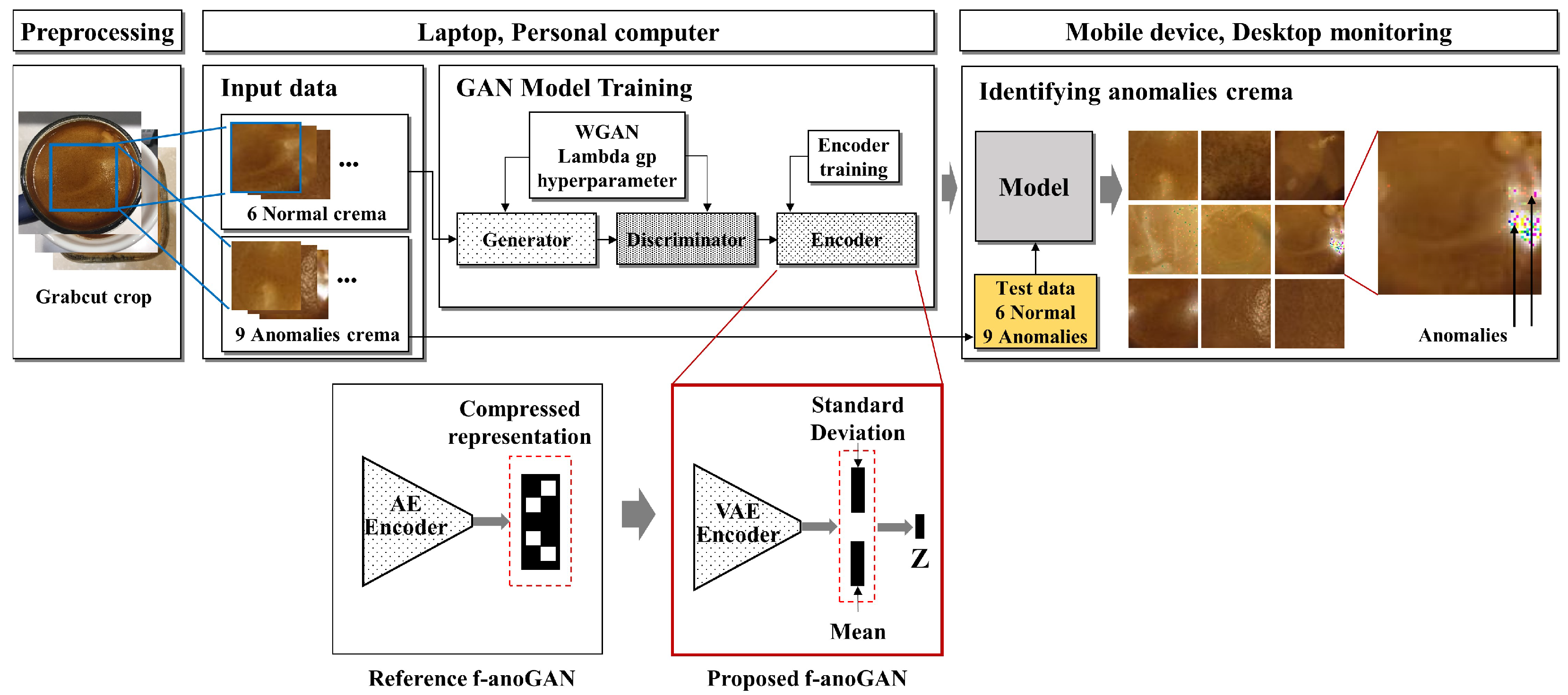
• Optimize the lambda gp hyperparameter in the combination of WGAN and VAE to enhance the performance in anomaly detection.

Through this research, our goal is to improve the accuracy and reliability of data in IoT systems and improve the efficiency of anomaly detection and data analysis. This will contribute significantly to the rapid and accurate detection of abnormal data in fields such as manufacturing, healthcare, and security.

Various important factors related to the essence of coffee and extraction methods [3,6,9], such as temperature, pressure, extraction time, grinding size, extraction volume, and bean aging, were discussed using image data from references [10] regarding the general result known as espresso crema. We classified the potential occurrences of normal and abnormal extraction methods that may arise when extracting espresso in a typical cafe. Figure 1a shows six normal data extracted correctly from a coffee machine, and (b) shows nine anomaly data classified as abnormal extraction. In this study, our objective is to design a system to enhance the efficiency of anomaly detection and data analysis using f-AnoGAN. To achieve this, we follow the overall workflow presented in Figure 2.

2. Related Work

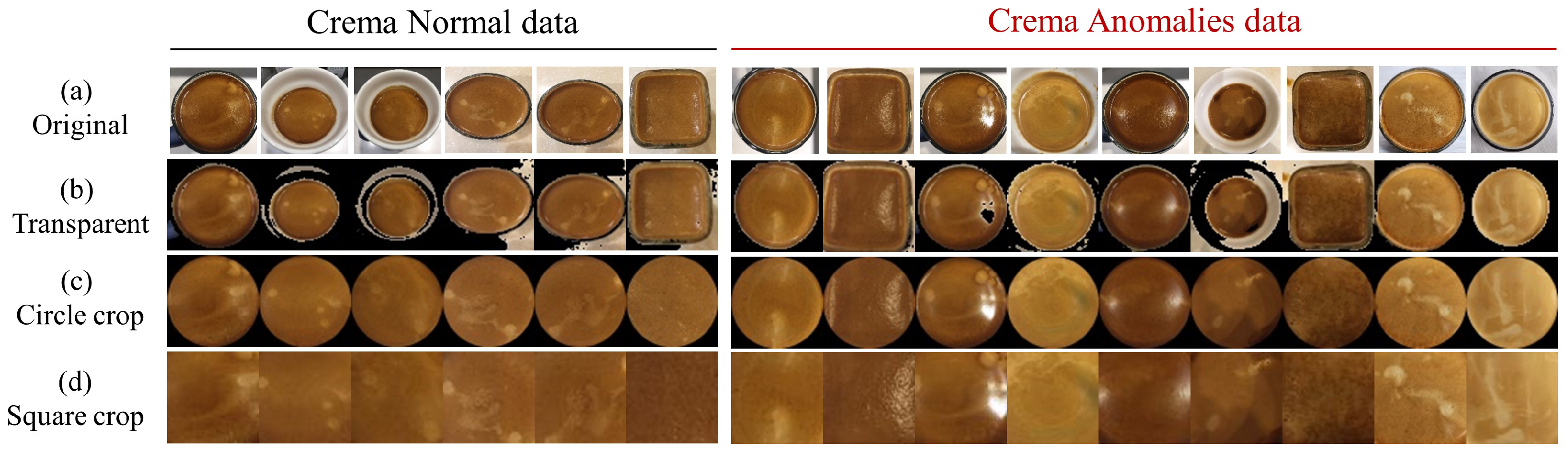
2.1. GrabCut Crop

The GrabCut algorithm (Interactive Foreground Extraction Using Iterated Graph Cuts) [11] effectively separates the foreground and background with minimal user input through an iterative optimization process. Although this approach allows for quick and efficient segmentation, it may not perfectly separate areas where colors meet. Traditional segmentation methods such as this can influence the accuracy of color clustering using K-means [12], potentially leading to imprecise results [10]. Therefore, this study adopts a GrabCut-based cropping method that allows users to directly separate images with ease. Although GrabCut is an older technique, it offers a compact approach that reduces hardware load, enabling the real-time adjustment of extraction parameters and ensuring consistent, high-quality image extraction. In this study, we combine GrabCut with f-AnoGAN for anomaly detection to establish a robust system to maintain espresso quality.

2.2. Generative Adversarial Network

Ian Goodfellow [13,14,15], the creator of generative adversarial networks (GANs), first proposed the concept by likening it to a game between a police officer and a counterfeiter. Here, the counterfeiter aims to produce counterfeit currency indistinguishable from real money to deceive the police, while the police endeavor to differentiate between genuine and counterfeit currency to apprehend the counterfeiter. In GANs, the generator aims to create data that resemble real data as closely as possible, while the discriminator aims to distinguish between real and fake data. Adversarial learning involves training the discriminator first and then training the generator repeatedly. The discriminator is trained on real images to classify them as real and on fake images generated by the generator to classify them as fake. Through this process, the discriminator becomes proficient in classifying real images as real and fake images as fake. As a result, the generator becomes adept at producing synthetic images that closely resemble real ones, making it challenging for the discriminator to differentiate between real and fake images. The generator’s goal is to reduce the probability of successful classification, while the discriminator aims to increase it, thus evolving competitively.

Our proposed research leverages the strengths of GAN-based anomaly detection techniques, specifically AnoGAN [12] and f-AnoGAN. Both approaches require mapping images to a latent space. However, due to the extremely small amount of data in our dataset, the Deep Convolutional Generative Adversarial Network (DCGAN) [16] used in AnoGAN and f-AnoGAN did not effectively map the images to the latent space through unsupervised learning of the generator and discriminator in normal data.

Since the introduction of the AnoGAN technique, there have been further applications of GAN-based anomaly detection. For example, a GAN-based communication fraud detection approach was proposed using a deep denoising autoencoder that learns the relationships between inputs and uses adversarial training to distinguish between positive and negative samples in the data distribution [17]. Furthermore, f-AnoGAN used the Wasserstein GAN (WGAN) [18] which improved the WGAN training procedure by replacing weight clipping with a Gradient Penalty [19].

In summary, while conventional f-AnoGAN was designed as a grayscale image-based model, our proposed research aims to address the challenges arising from similar color images and limited data constraints by leveraging the strengths of existing GAN-based anomaly detection methods [20]. Specifically, we propose a novel approach that improves the architecture of the generator and discriminator and optimizes the lambda_gp hyperparameter during the training process. Notably, we introduce VAE to learn the latent space representation of color images and alleviate the data scarcity problem by adding the reconstruction error of VAE as a regularization term. The experimental results demonstrate that our proposed model outperforms the conventional f-AnoGAN model by 0.13 in terms of the Receiver Operating Characteristic Area Under the Curve (ROC-AUC) metric, validating its effectiveness in the detection of anomalies based on color images.

2.3. Autoencoder- and Variational Autoencoder-Based Generative Model

An autoencoder (AE) [21,22,23,24] is a network that encodes the input data in a low-dimensional latent space and then decodes them back into the original input data. When used as a generative model, an AE takes sampled points from the latent space as input and decodes them into original data, generating new data. Autoencoder-based generative models such as Variational Autoencoder (VAE) can produce diverse results during the sampling process in the latent space. An AE is characterized by having fewer nodes in the hidden layer (also called the bottleneck layer) than the input value, serving as a simple neural network that merely copies the input to the output. Hence, one might expect the input and output to be identical images. The reason for using the method of copying the input to the output is due to the hidden layer. The bottleneck layer of an AE has far fewer neurons than the input and output. In other words, the AE is the best way to represent data with a small number of neurons in the bottleneck layer.

An AE is a neural network that is used to compress data into a latent representation and then reconstruct them back to the original data (Figure 3a). An AE consists of two main components: It encodes the input data x into a latent variable z. The encoder network outputs a predicted latent variable $\widehat{z}$. The decoder reconstructs the original data x from the latent variable $\widehat{z}$. The decoder network takes the latent variable z as input and outputs the reconstructed data $\widehat{x}$. The goal of AE is to minimize the difference between the input data and the reconstructed data. This goal can be expressed mathematically as Equation (1):

$${Loss}_{AE}={\parallel x-\widehat{x}\parallel }^2$$

(1)

where ${\parallel ·\parallel }^2$ typically represents the Euclidean distance (or mean square error). This loss function trains the AE to minimize the difference between the input and the reconstructed data. Autoencoders have emerged as a cornerstone of machine learning, offering a versatile toolkit for tasks ranging from data compression to feature extraction. Their ability to learn compressed representations of data has proven invaluable in various applications.

Variational Autoencoders (VAEs) are a type of generative model that learn to model the distribution of data and generate new samples from that distribution. They extend the basic AE concept by incorporating probabilistic elements to create a more flexible and powerful generative model.

• Encodes the input data x into a probability distribution $q(z\mid x)$ over latent variables z. Typically, this distribution is parameterized by a mean $\mu$ and variance ${\sigma }^2$. The encoder outputs the mean $\mu$ and variance ${\sigma }^2$. To sample from the latent variable, the reparameterization trick is used: $z=\mu +{\sigma }^2·ϵ$ (where $ϵ$ is sampled from a standard normal distribution).
• Reconstructs the original data x from the latent variable z. The decoder network takes z as input and outputs the reconstructed data $\widehat{x}$.
• VAE loss function consists of two parts:
• Measures the difference between the input data and the reconstructed data (Equation (2)).

  $$\mathrm{Reconstruction}\mathrm{Loss}=\parallel x-\widehat{x}{\parallel }^2$$

  (2)
• Divergence: Measures the difference between the latent variable distribution of the encoder $q(z\mid x)$ and the previous distribution $p\left(z\right)$ (usually a standard normal distribution) (Equation (3)).

  $$\mathrm{KL}(q(z\mid x)\parallel p\left(z\right))={\displaystyle \frac{1}{2}}\sum _{i=1}^D\left({\sigma }_i^2+{\mu }_i^2-log\left({\sigma }_i^2\right)-1\right)$$

  (3)
• Total loss function for VAE is as follows (Equation (4)):

  $${Loss}_{VAE}=\mathrm{Reconstruction}\mathrm{Loss}+\mathrm{KL}\mathrm{Divergence}$$

  (4)
• Loss function trains the VAE to both reconstruct the data well and ensure that the latent variable distribution resembles the prior distribution.

VAE can generate new data by sampling from the latent space and has stronger generalization capabilities by modeling the probabilistic distribution of the data. It effectively captures the complex structure of the data and can model a variety of distributions. Due to these advantages, VAE is widely used in various fields, such as image generation, data augmentation, and anomaly detection (Figure 3b).

2.4. f-AnoGAN

F-AnoGAN [25] is a GAN-based model that is used primarily for anomaly detection. The original AnoGAN uses a generator and a discriminator to learn and detect anomalous data. F-AnoGAN is an optimized version designed to perform this task more quickly.

AnoGAN is efficient and fast when the training image size is small. However, as the image size increases, the method’s random iteration approach can lead to inadequate mapping because of the need to consider a larger amount of information. To address this issue, f-AnoGAN took inspiration from AE. An AE is a simple model that compresses input information into a latent vector that effectively describes it and then reconstructs it through a decoder. The core of f-AnoGAN is using the AE model to map images to the latent space. By doing this, the process of mapping training data (normal images) to the latent space can be viewed as an identity transformation. In essence, f-AnoGAN uses the encoder of an AE to perform image-to-latent space mapping more efficiently and accurately, thus addressing the shortcomings of AnoGAN.

As in Equations (5) and (6), this paper largely adopts f-AnoGAN. In the f-AnoGAN paper, to address the issue of improper mapping when a query image is input, the authors devised a method to optimize the WGAN’s Gradient Penalty (GP) parameter, thereby improving the final anomaly score and increasing the AUC value.

$${\mathcal{L}}_{izi}\left(\mathbf{x}\right)={\displaystyle \frac{1}{n}}{\parallel \mathbf{x}-G\left(E\left(\mathbf{x}\right)\right)\parallel }^2$$

(5)

$${\mathcal{L}}_{iz{i}_f}\left(\mathbf{x}\right)={\displaystyle \frac{1}{n}}{·\parallel \mathbf{x}-G\left(E\left(\mathbf{x}\right)\right)\parallel }^2+{\displaystyle \frac{\kappa }{n_d}}·{\parallel f\left(\mathbf{x}\right)-f\left(G\left(E\left(\mathbf{x}\right)\right)\right)\parallel }^2$$

(6)

• The Gradient Penalty was introduced in WGAN-GP (Wasserstein GAN with Gradient Penalty). In conventional GANs, training instability can be an issue. WGAN improves stability by using the Wasserstein distance. However, WGAN must enforce the Lipschitz continuity by ensuring that the discriminator gradient does not exceed 1. The Gradient Penalty is introduced to enforce this Lipschitz continuity. It does so by penalizing the discriminator’s gradient norm, encouraging it to stay close to 1, which helps to achieve more stable training.

The role of lambda_gp is the parameter that represents the weight of the Gradient Penalty term. This parameter determines how strongly the penalty is applied to the gradient of the discriminator.

The Gradient Penalty term penalizes the discriminator’s gradient norm in proportion to how much it deviates from 1. lambda_gp controls the strength of this penalty. A higher value enforces a stronger penalty, pushing the gradient closer to 1.

Adjusting the value lambda_gp, one can control the stability of the training of the model. A value that is too low may not sufficiently enforce Lipschitz continuity, leading to unstable training. In contrast, a value that is too high might impose excessive constraints, slowing down the learning process or making it difficult to find the optimal solution.

In f-AnoGAN, the parameter lambda_gp plays a crucial role in controlling the strength of the Gradient Penalty. This ensures that the discriminator’s gradient norm remains close to 1, enhancing the training stability and improving the model’s performance in anomaly detection. Selecting an appropriate lambda_gp value is essential for a successful training of f-AnoGAN.

3. Experiment

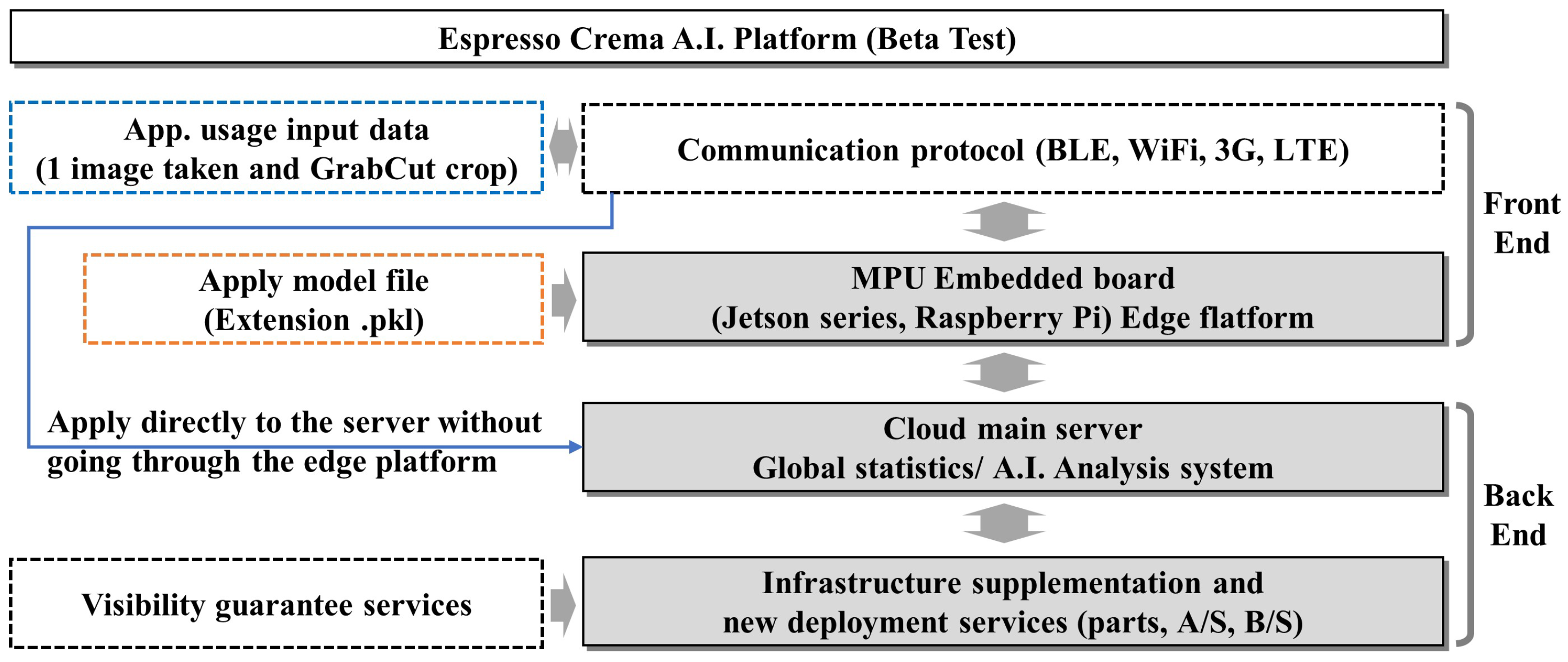
3.1. Overall Design

We propose an anomaly detection technique to evaluate images of coffee crema extracted from an actual coffee machine, focusing on both under-extracted and over-extracted data. The primary goal of this study is to determine whether the model can classify realistic images extracted from a coffee machine, identify anomalies in the extraction process, and accurately highlight anomaly regions. To verify the precision of the anomaly scores of the proposed approach with a limited dataset, we compare it with the DCGAN + AE and VAE models. To ensure robust segmentation under various lighting and background conditions, additional preprocessing methods and coffee crema data are referenced from [10], and we also compare the proposed f-AnoGAN, based on the WGAN presented in [12,25], to analyze the data from a small number of images. Given that basic parameter settings are insufficient for analyzing a limited number of images, we optimize the parameters to effectively evaluate performance. The proposed anomaly detection technique is based on realistic images of coffee crema extracted from an actual coffee machine, assessing the model’s ability to classify normal and abnormal data. This involves evaluating the ability of the machine learning model to learn the characteristics of each image and distinguish between normal and abnormal crema. Furthermore, we investigate whether the model can accurately identify anomalies in the extracted images and highlight the corresponding regions clearly. This study compares the anomaly detection performance of the proposed method with that of the DCGAN + AE and VAE models to validate the superiority of the proposed methodology. In particular, the ability of the f-AnoGAN model to effectively analyze a small number of image data is assessed by optimizing various parameters to accurately measure performance. This study aims to propose an effective model for the anomaly detection and classification of coffee crema images, and, by comparing it with various existing models, to demonstrate the performance and validity of the proposed approach. We conduct experiments to validate the model for each system and the key parameters are as follows.

• Desktop i7: Windows 11, Intel(R) Core(TM) i7-8700 CPU 3.2 GHz, DDR4 32GB;
• Laptop i7: Windows 10 Pro, Intel(R) Core(TM) i7-10510U CPU 1.8 GHz, DDR4 16GB;
• Nvidia Jetson Nano (B01): Ubuntu 20.04, Quad-core ARM Cortex A57 1.43 GHz, LPDDR4 4GB, 64GB microSD, disable CUDA;
• Nvidia Jetson NX: Ubuntu 20.04, 6-core Nvidia Carmel ARM v8.2 2-core 1.9GHz, LPDDR4 8GB, 128GB SSD, disable CUDA;
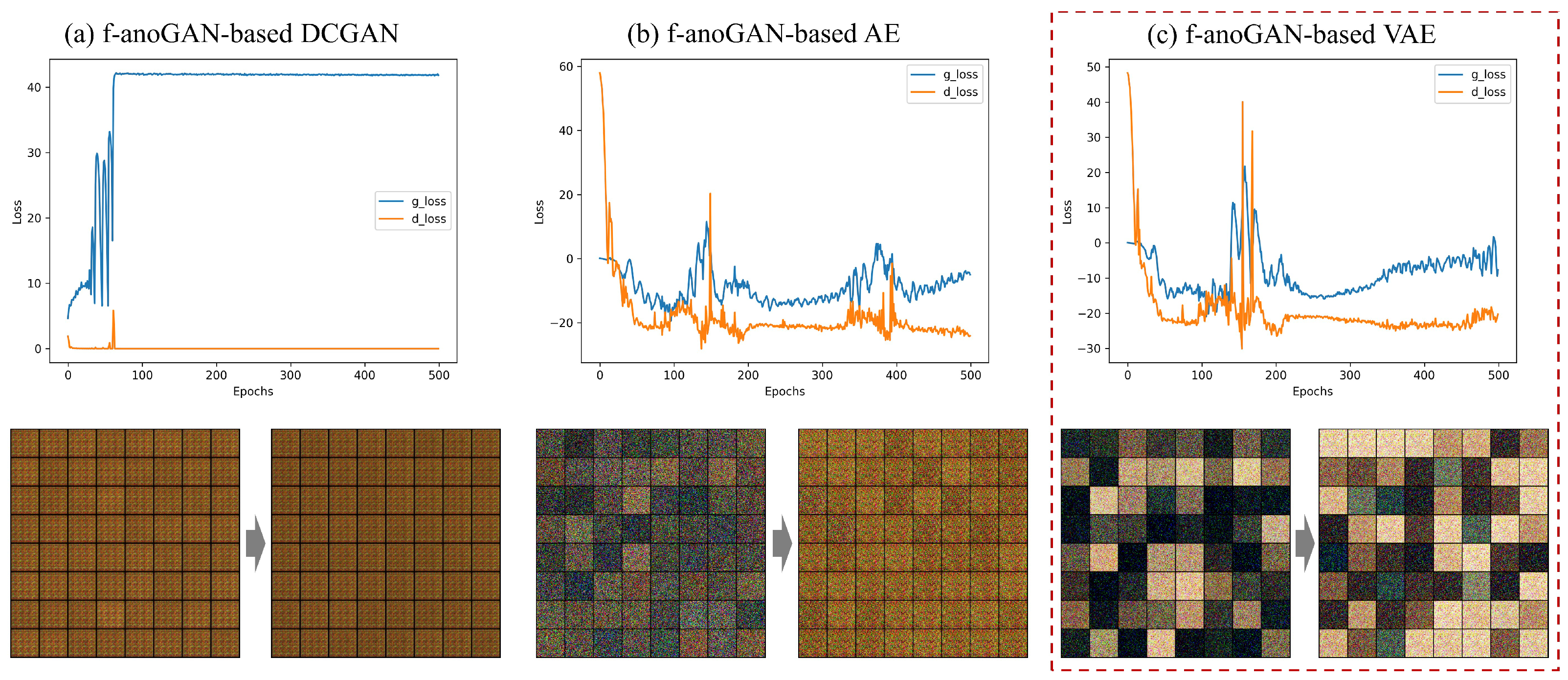
• Model parameters: epochs = 500, batch size = 128, lr = 0.0002, b1 = 0.5, b2 = 0.999, latent dim = 100, img size = 64, channels = 3, n critic = 5, sample interval = 400, training label = 0, lambda gp = 50, weight decay = 0.00005, Adam optimizer.

On the desktop, two functions are performed: generating and evaluating the model. The Windows experiment environment is conducted using Microsoft Visual Studio Code, Python 3.8.1, and the Pytorch library (2.2.1 + cpu). The Jetson series environment also uses Microsoft Visual Studio Code, Python 3.8.1, and the Pytorch library (Nano 1.12.0, NX 2.0.1 + cpu) for the experiments (Figure 4). These environments ensure consistency and reliability in the experiments. This methodology allows for the accurate measurement of the system performance and the verification of its applicability in real-world scenarios.

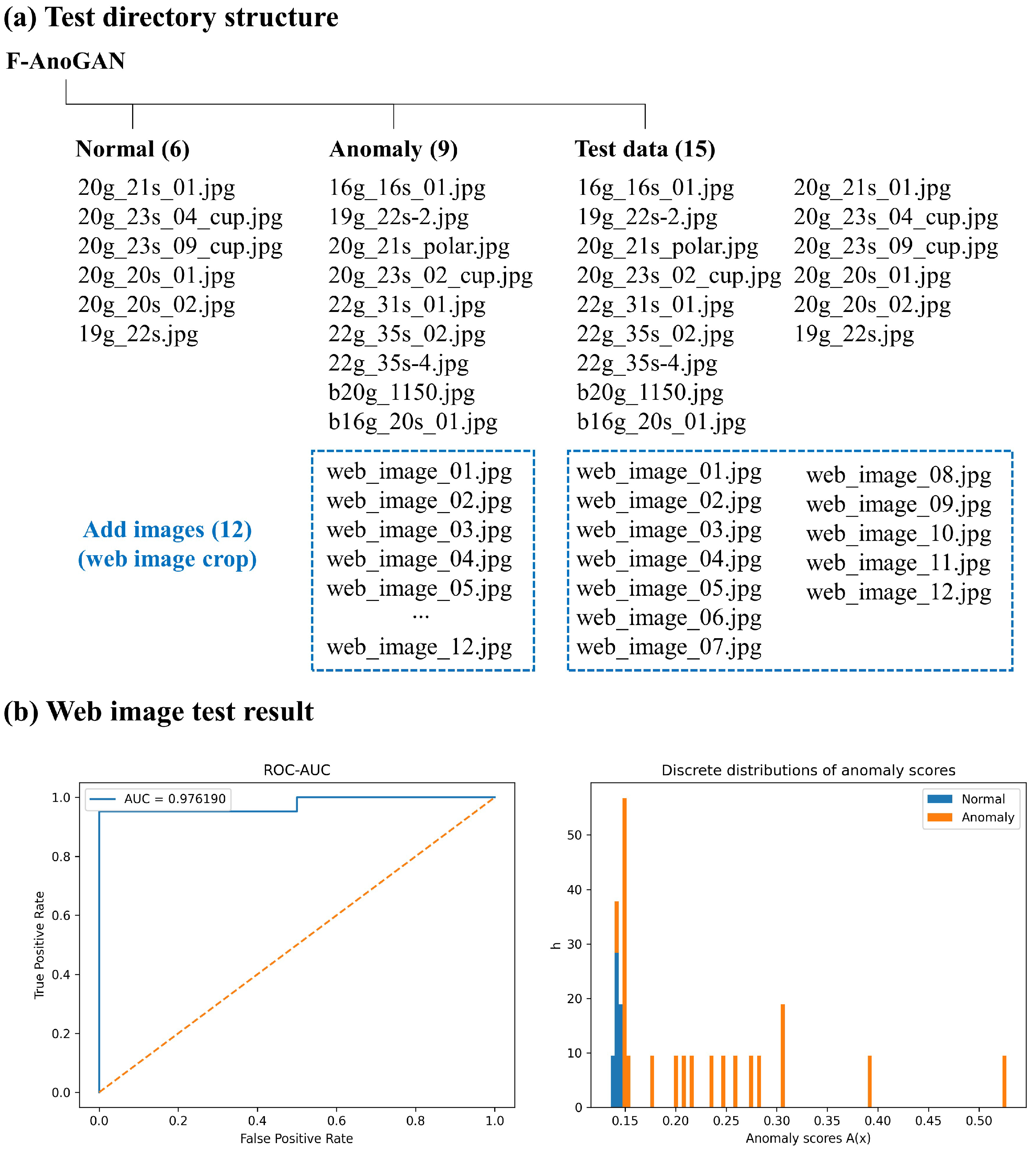
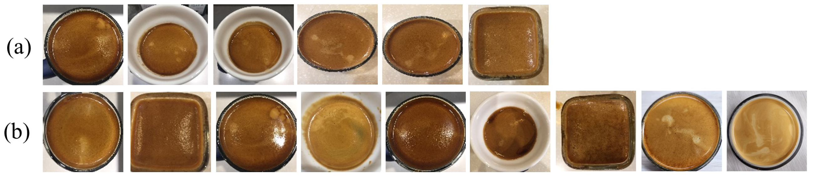
3.2. Data Selection and Preprocessing

The goal of this study was to achieve a real-time system with deep learning methods using a small amount of data, centered on user interaction, that operates at the same speed as machine learning. We adopted a semi-supervised approach to distinguish between normal (six images) and abnormal (nine images) crema images captured by users. To facilitate comparison, we used the GrabCut transparent segmentation algorithm described in [10] to segment and store the crema regions of various cups. In addition, we extracted the GrabCut crop in two different ways for further comparison in this experiment. We examined which method is more suitable for real-time analysis by cropping and saving only the black background and the actual crema region that occurred during GrabCut.

In the real-time image data processing and deep learning system, high-resolution images cannot be analyzed. To utilize high-resolution images captured by mobile phones for deep learning model training, all images were resized to a uniform size of $64\times 64$ pixels. This adjustment is optimal for edge computing in building an automated system aimed at reducing wireless network transmission costs and enhancing quick response capabilities. The images were captured and stored with a smartphone camera in a square format with a 1:1 aspect ratio to minimize distortion and unwanted background. Through this process, the captured crema images are appropriately formatted and optimized in the Jetson series, allowing an efficient and effective evaluation of crema quality.

We assumed a scenario where the model was developed in a general Personal Computer (PC) environment, and photos taken by a mobile device were preprocessed using our proposed GrabCut crop algorithm and then transmitted by the user. We aim to minimize manual data preprocessing methods and apply a lightweight and fast approach (Figure 5). When the user sent a photo taken with a smartphone, we applied a data processing method that effectively used f-AnoGAN to detect anomalies in the crema portion within the Nvidia Jetson series. This simplified the preprocessing process and enabled direct user services using edge computing.

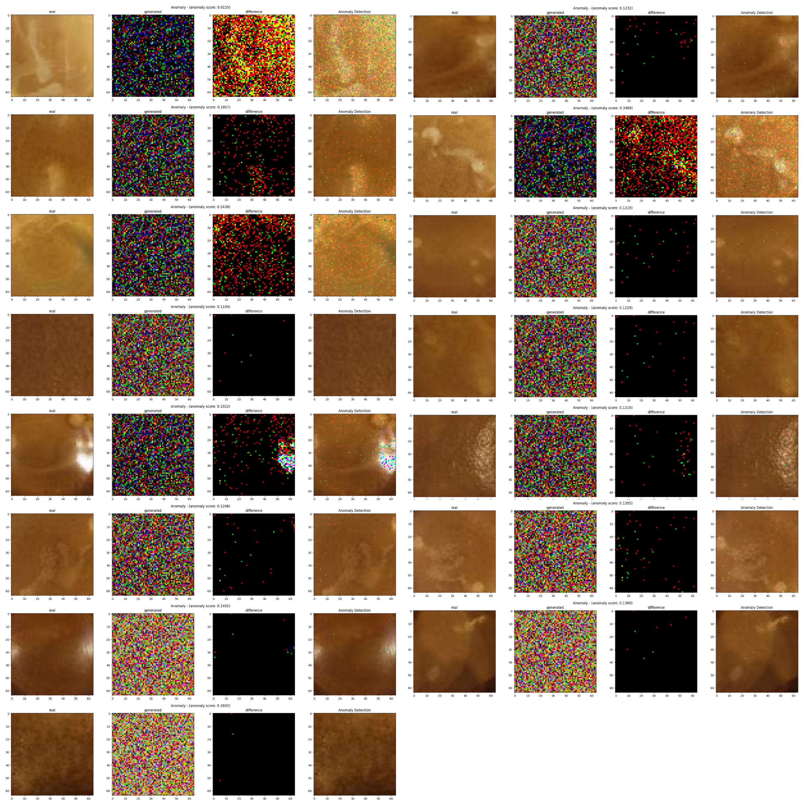
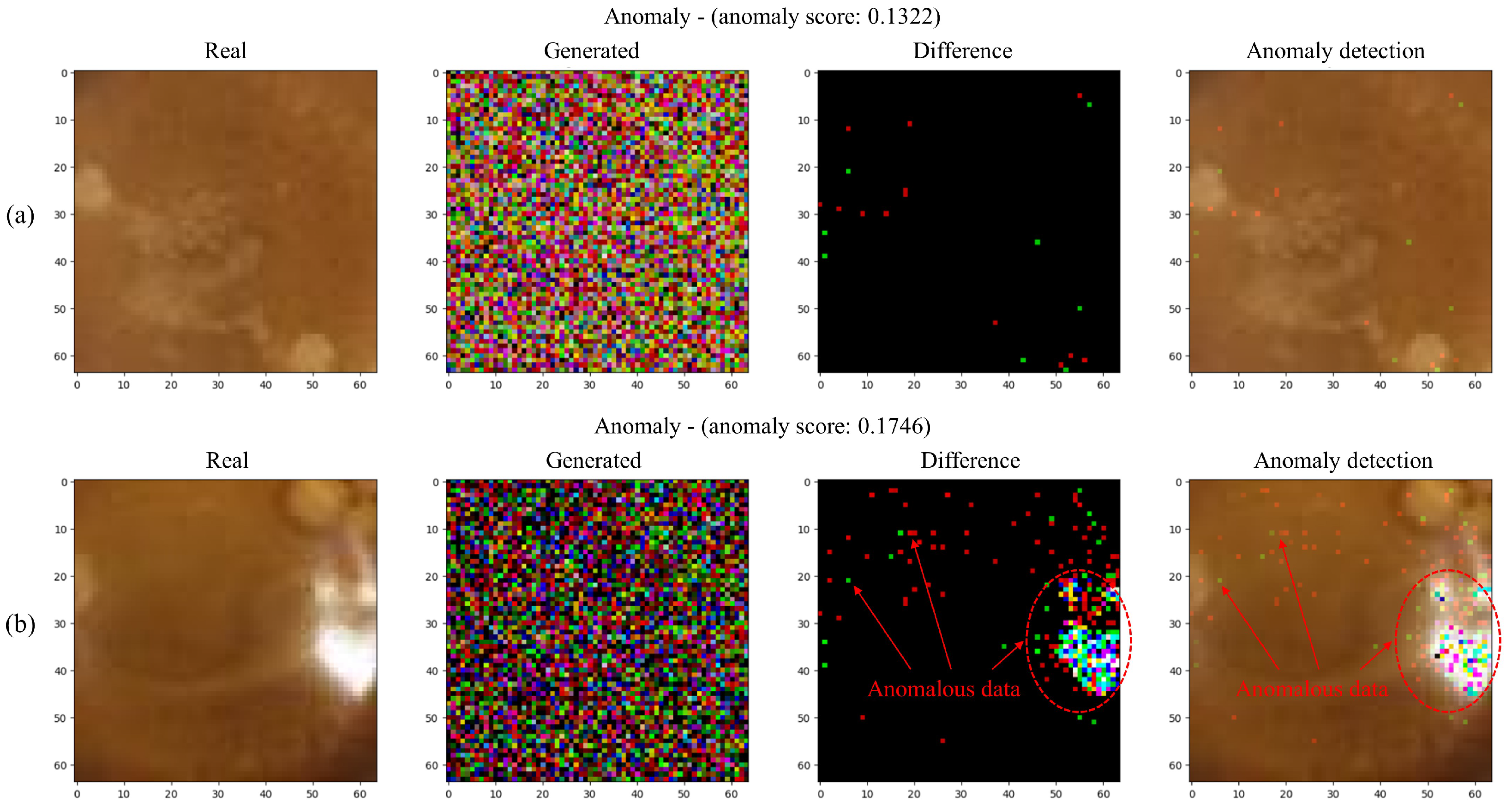
3.3. Evaluation Using Anomaly Score

We conducted experiments using f-AnoGAN to evaluate the performance of various combinations of models and parameter settings. The primary objectives of these experiments were to assess the training performance of the DCGAN, VAE, and AE models, to analyze the impact of the optimal parameter setting (lambda_gp) for the WGAN model, to measure the iterative accuracy of the model using the Pearson correlation coefficient, and to evaluate the final performance of the f-AnoGAN anomaly score for the detection of anomalies. Firstly, we compared the performance of training using different combinations of the Deep Convolutional Generative Adversarial Network (DCGAN), VAE, and AE models. This involved closely monitoring each model’s convergence speed, quality of the generated samples, and training stability. Next, we optimized the performance of the WGAN model by adjusting the lambda_gp (Gradient Penalty) parameter. We evaluated how changes in the lambda_gp value affected the model learning performance and sample quality, ultimately determining the optimal value of lambda_gp. In addition, we analyzed the iterative accuracy of the models by calculating the Pearson correlation coefficient. This metric allowed us to assess how consistently the model produced results and to compare the performance of models with different levels of consistency. Finally, we evaluated the performance of anomaly detection using f-AnoGAN by measuring the anomaly score. This assessment helped us understand how effectively f-AnoGAN differentiates between normal and anomalous data, and we analyzed the precision and reliability of the final anomaly score. Through these experiments, our objective was to gain a comprehensive understanding of how various combinations of models and parameter settings affect the performance of f-AnoGAN and to assess its utility in anomaly detection.

Comparing DCGAN, VAE, and AE models in f-AnoGAN: Can more complex algorithms better identify anomaly images? Unlike traditional deep learning, which requires tens of thousands of data points, real-life applications of AI and deep learning often have limited data. To improve the accuracy in such cases, we conducted extensive testing to determine optimal parameters and compared DCGAN, VAE, and AE. We found that DCGAN, although expected to perform better, did not converge well with small datasets. This highlights the importance of choosing and adjusting algorithms and parameters according to the specific situation rather than always opting for the most complex one. Through this comparative evaluation of the models, the method proposed in this study proved to be effective. The graph visually represents the error between the generator and the discriminator (Figure 6).

Optimal parameters for the WGAN model: In this paper, we propose a method to optimize the Gradient Penalty (GP) parameter of WGAN. This addresses the issue of improper mapping when a query image is input and improves the final anomaly score’s AUC value. The proposed method improves model training stability and mitigates gradient explosion and vanishing problems, providing better performance. Wasserstein GAN with Gradient Penalty (WGAN-GP) is a model proposed for the stable training of generative adversarial networks (GANs), aiming to solve the mode collapse issue inherent in traditional GANs. This study analyzes the code for calculating the Gradient Penalty, a core component of the WGAN-GP model, and performs experimental research to determine the optimal model parameter settings. WGAN training involves using the adaptive moment estimation optimizer (Adam) [26] for the generator, discriminator, and encoder.

Repeated accuracy of the model: The primary goal of this paper was to design a system that provides visual information in real time to users and to implement this system effectively. To achieve this, our objective was to verify the accuracy of the system as it provides continuous data. This precision is crucial in processes that impact manufacturing and productivity. Using Google Colaboratory, we executed the basic code and completed the f-AnoGAN model code, saving it for future use. The saved models for the generator, discriminator, and encoder were stored as two Python pickle (pkl) files, enabling their use in various systems in real time.

3.4. Experimental Results

As demonstrated in the f-AnoGAN paper, low-resolution grayscale MNIST [27] images can be effectively trained without additional parameter tuning, resulting in high AUC performance. To apply f-AnoGAN to color images, such as crema images, we first performed preliminary experiments using the CIFAR-10 dataset [28]. Although the conventional f-AnoGAN model achieved an AUC of 0.39 in CIFAR-10, our proposed VAE-based f-AnoGAN model showed an improvement of 0.13, reaching 0.52. However, the overall blurriness of the images in the CIFAR-10 dataset led to a relatively lower AUC. However, the espresso crema images used in this study achieved an AUC performance of 0.98. Additionally, to improve reliability and broaden applicability beyond data from a single café, 12 anomaly images were cropped from a free online image site and added to the dataset for extended testing. As a result, there was a slight performance drop (AUC: 0.976), but it was not significant. The detection results for crema images of entirely different colors remained excellent. The directory structure and results of the expanded dataset are presented in Figure A2 of Appendix B.

In this study, we conducted various experiments to improve the anomaly detection performance using f-AnoGAN. First, we analyzed the impact of the optimal parameter, $lambda\_gp$, in the WGAN model on the anomaly detection performance using

Table 1. The table compares the performance of the AE and VAE models based on different $lambda\_gp$ values in the WGAN model across three GrabCut methods: (a) transparent, (b) circle crop, and (c) square crop. The AE model shows peak performance at specific $lambda\_gp$ values (40, 50, 60), but its performance decreases if $lambda\_gp$ is too high or too low. However, the VAE model maintains a more consistent performance, with the highest values observed at $lambda\_gp$ of 30, 40, and 50, indicating less sensitivity to changes in $lambda\_gp$ compared to AE.

Model	Grabcut	WGAN lambda gp Parameter
		30	40	50	60	70
AE	(a) Transparent	0.6852	0.8519	0.6481	0.8148	0.6111
	(b) Circle crop	0.8704	0.6481	0.8889	0.6111	0.6296
	(c) Square crop	0.8148	0.7778	0.6296	0.9630	0.9074
VAE	(a) Transparent	0.8889	0.8704	0.7222	0.8704	0.8704
	(b) Circle crop	0.8889	1.0000	1.0000	0.9444	0.8889
	(c) Square crop	0.9259	1.0000	1.0000	0.9815	0.7407

. Furthermore, we compared and evaluated the performance of f-AnoGAN through combinations with various generative models such as DCGAN, VAE, and AE, as shown in

Table 2. This summarizes the performance comparison across various model combinations by adjusting the $lambda\_gp$ hyperparameter in WGAN. The key comparisons are between four combinations: DCGAN and f-AnoGAN structures paired with AE and VAE models. DCGAN+AE (a): Showed the highest performance (0.6296) when $lambda\_gp$ was set to 50. Overall, the performance was lower compared to other combinations, with only slight variations in performance as $lambda\_gp$ changed. DCGAN + VAE (b): achieved the highest performance (0.7222) at a $lambda\_gp$ of 70, with a general trend of increasing performance as $lambda\_gp$ increased. f-AnoGAN + AE (c): recorded the highest performance (0.9630) at a $lambda\_gp$ of 60, showing generally high performance, but with a decrease when $lambda\_gp$ was too low or too high. f-AnoGAN+VAE (d): achieved perfect performance (1.0000) at $lambda\_gp$ values of 40 and 50, indicating optimal performance when $lambda\_gp$ is between 40 and 50.

Model	WGAN lambda gp Hyperparameter
	30	40	50	60	70
(a) DCGAN+AE	0.5741	0.5556	0.6296	0.5370	0.5926
(b) DCGAN+VAE	0.5741	0.5741	0.5741	0.5926	0.7222
(c) f-AnoGAN+AE	0.8148	0.7778	0.6296	0.9630	0.9074
(d) f-AnoGAN+VAE	0.9259	1.0000	1.0000	0.9815	0.7407

. Furthermore, we measured the final anomaly score of the anomaly detection model using f-AnoGAN in a real-world application environment to verify its performance. In the experimental setup shown in Figure 4, the Pearson correlation coefficient is used to validate how accurately the model outputs values without distortion when a crema image is input. Although the Pearson correlation coefficient itself may not carry significant meaning, evaluating the repeatability of the model with minimal error allowed us to confirm the feasibility of using artificial intelligence within the system.

According to the results in Table 1, the AE model showed varying AUC values depending on the characteristics of the image, while the VAE model exhibited stable AUC values regardless of the characteristics of the image. This indicates that the VAE model learns more general features than the AE model. In the case of the WGAN model, our aim was to optimize the performance of the model by adjusting the parameter $lambda\_gp$. The experimental results showed that the training performance of the model and the quality of the generated samples varied significantly depending on the value of $lambda\_gp$. Specifically, when the value of $lambda\_gp$ was too small, the model tended to overfit, resulting in a decrease in the diversity of the generated samples. In contrast, when the value of $lambda\_gp$ was too large, the model tended to fit poorly, leading to a degradation in the quality of the generated samples. Through various experiments, we found that setting the $lambda\_gp$ value between 40 and 60 yielded the best performance. In other words, proper adjustment of the value of $lambda\_gp$ is a crucial factor in determining the performance of the WGAN model, and the balance between overfitting and underfitting is essential. The results of this study provide important insight into parameter tuning for WGAN models and are expected to contribute to future research using WGAN models.

Table 2 presents a comparison of the results obtained by training various combinations of the DCGAN, VAE, and AE models. The models were evaluated on the basis of the convergence speed, the quality of the generated samples, and the training stability. In general, models based on f-AnoGAN exhibited the highest performance, with the combination f-AnoGAN + VAE demonstrating superior performance in all values of $lambda\_gp$. In contrast, DCGAN-based models showed relatively lower performance, with the DCGAN + AE combination performing the worst. Although the parameter $lambda\_gp$, introduced in WGAN to enhance the stability of the model, was found to have a limited impact on the performance of the model in our experiments, the combination of f-AnoGAN + VAE achieved the best performance when the value $lambda\_gp$ was set to 40 or 50, indicating that these values are optimal for this specific combination of models. DCGAN is a type of GAN commonly used for image generation, VAE is a model that generates data using latent variables, and AE is an autoencoder model that compresses and reconstructs data. This study evaluated the performance of f-AnoGAN by combining these various models and analyzed the impact of the parameter $lambda\_gp$.

As introduced in the paper, f-AnoGAN is an improved version of existing AnoGAN (Anomaly GAN). It first trains a GAN using normal data to learn the latent space of the data. Then, it performs anomaly detection by calculating the difference between the input data and the reconstructed data using an autoencoder (AE) or Variational Autoencoder (VAE). AE and VAE learn the normal patterns during the process of compressing and reconstructing the input data.

Training with normal data: The GAN is trained only with normal data, which allows it to learn normal patterns. Latent Space Exploration: For given input data, the most similar latent space vector is identified. AE or VAE is used in this process to reconstruct the input data based on this vector. Reconstruction error calculation: The difference (error) between the input data and the reconstructed data is calculated. For normal data, this error is small but, for anomalous data, the error is significantly larger. Calculation of anomaly score: An anomaly score is computed on the basis of this reconstruction error. If this score exceeds a certain threshold, the data are classified as anomalous.

The anomaly detection performance of f-AnoGAN is evaluated using metrics such as accuracy, precision, recall, and the F1 score. Accuracy represents the proportion of correctly classified normal and anomalous data, precision indicates the ratio of actual anomalous data among those predicted as anomalous, and recall measures the proportion of actual anomalous data correctly identified by the model. The paper evaluates the model’s performance using the Area Under the Curve (AUC). AUC represents the area under the ROC curve, with values closer to 1 indicating better performance. Figure 7 shows representative results for (a) normal and (b) anomaly data. These difference and anomaly detection result images can be presented visually to users immediately. In addition, the anomaly score is provided in text format, which facilitates integration with various applications, improving its usability. The test results for the entire dataset are presented in Figure A1 of Appendix A. In Figure 7 and Figure A1, the visual analysis of anomalies shows that, in the “Difference” column, the closer the background color is to black, the more it indicates a normal image. Conversely, the presence and distribution of various colors, such as red, green, blue, and white, signify areas of abnormality (irregular crema regions). Similarly, the visualizations in the “Anomaly Detection” column indicate that parts of the coffee crema background containing or exhibiting a significant distribution of diverse colors represent areas of abnormality (irregular crema regions).

To analyze the repeatability accuracy of the model, Pearson’s correlation coefficients were calculated. This helped evaluate how consistently the model generates results over multiple runs. The model was created using Google Colaboratory on a desktop and saved in the .pkl file format. Python’s pickle library supports the serialization and deserialization of objects, allowing Python objects to be stored in files and restored as needed. Subsequently, the generator, discriminator, and encoder files, along with normal and anomaly crema image data, were copied to three different systems. The anomaly scores were then checked sequentially using Visual Studio Code and the Jupyter notebook. Using the anomaly scores measured on the desktop as a baseline, a total of 15 datasets were classified on four systems: desktop, laptop, Jetson Nano, and Jetson Xavier NX. Pearson’s correlation coefficients were calculated on the basis of the anomaly scores of these datasets.

Table 3. This table compares the running times of models on various system devices. The table is divided into two main categories: “Cold Start” and “Standard Start”. Cold Start refers to the time when the Python module was not imported by executing the Visual Studio Code for the first time, and Standard Start refers to the execution of the program while the module is imported. A test load image refers to the point in time when the crema image is imported and executed from the test data folder.

System Device	Model Execution Time
	Cold Start		Standard Start
	Full	Test Load Image	Full	Test Load Image
Desktop i7	7.6 s ± 1.43	1.5 s ± 0.06	2.1 s ± 0.01	1.5 s ± 0.02
Laptop i7	7.8 s ± 0.18	2.0 s ± 0.06	2.7 s ± 0.04	2.0 s ± 0.04
Jetson Nano	105.4 s ± 10.14	36.9 s ± 9.54	45.0 s ± 4.09	17.3 s ± 2.68
Jetson NX	36.0 s ± 4.22	20.4 s ± 2.77	22.3 s ± 1.60	18.7 s ± 1.68

presents the Pearson correlation coefficients for the four different systems, showing that the proposed f-AnoGAN algorithm demonstrates a strong positive correlation with r = 0.999 or higher in all systems. This confirms the accuracy and error rate of the algorithm.

Table 3 shows the results of the timing analysis, which is a crucial concept to evaluate whether the artificial intelligence model we are using is suitable for the design and analysis of real-time systems. To calculate the Worst-Case Execution Time (WCET) for each system, we ran the Visual Studio Code program five times and obtained the results.

Delay analysis assesses whether a system can complete tasks in a specified time frame. For response time analysis, we conducted two evaluations: Cold Start and Standard Start. As shown in Table 3, a general single-board computer (SBC), even without a GPU, is expected to be utilized for artificial intelligence systems. This analysis helps verify whether tasks are completed within their deadlines, providing valuable insight for system device design.

3.5. Discussion

Figure 8 illustrates the discrete distribution of anomaly scores generated by the f-AnoGAN model using images of espresso crema. The red dashed box in these graphs is of significant importance. It demonstrates a critical fact: the f-AnoGAN algorithm, optimized for image data analysis, can be communicated in text form to control various other devices, which highlights its potential for broader applications. When normal and anomaly data overlap, as seen in (b), it becomes challenging to create a reliable control constant table. This issue is particularly relevant when considering the large portion of crema that involves the settings of the coffee grinder. For future applications involving connected AI systems to control devices such as motors, it is crucial that the anomaly scores are well separated, as shown in (a), to ensure precise control. The application of the Variational Autoencoder (VAE) to enhance the f-AnoGAN model in this study is particularly notable. This further underscores the importance of the proposed method in accurately identifying the distribution of crema images, proving the robustness of VAE-enhanced f-AnoGAN in anomaly detection. The analysis in (b) represents the traditional method for analyzing the f-AnoGAN models, where the model was tuned to achieve the highest Receiver Operating Characteristic Area Under the Curve (ROC-AUC) value of 0.963, indicating the best performing parameters. In summary, the proposed algorithm demonstrates its ability to accurately distinguish between normal and anomalous crema images, which is essential for precise control in AI-driven applications. This advancement could pave the way for more reliable and efficient AI applications in various fields, particularly those involving connected devices and real-time control systems. Figure A3 in Appendix C suggests the potential for expansion in applications, such as the integration of AI systems and mobile devices, through examples of communication protocols, system architecture, and the use of cloud services.

Table 4. The results of comparing the performance of two models (DCGAN+AE, DCGAN+VAE) across various hyperparameter values are as follows: (a) Weight initialization parameter: This parameter sets the initial weights during model training, with the highest performance observed at 0.03. Performance tends to decrease as the parameter value increases. (b) WGAN lambda gp hyperparameter: a specific hyperparameter for the WGAN-GP model, where the performance of the VAE used in this study remained similar across all parameter values, showing no significant differences.

Model	Weight Initialization Parameter
	0.02	0.03	0.04	0.05	0.06
(a) DCGAN+AE	0.3897	0.4811	0.4476	0.4373	0.3446
Model	WGAN lambda gp hyperparameter
	30	40	50	60	70
(b) DCGAN+VAE	0.5251	0.5249	0.5250	0.5261	0.5267

and related results show the performance limitations of the DCGAN algorithm. To address these, WGAN [18] introduced a new loss function based on Wasserstein distance, enabling more stable training. Unlike the binary cross-entropy loss in DCGAN, which often leads to mode collapse (where the model generates only a few repetitive images), WGAN’s loss function mitigates this issue by providing a meaningful measure of distance between probability distributions. This improvement enhances the diversity and realism of generated images. f-AnoGAN builds on WGAN’s strengths, applying its principles to anomaly detection. By leveraging WGAN’s stable training process and effective loss function, f-AnoGAN learns normal data distributions and detects anomalies more reliably. Specifically, f-AnoGAN benefits from WGAN’s two key contributions: (1) a Wasserstein distance-based loss function that stabilizes training and resolves mode collapse, and (2) improved training dynamics for both the generator and discriminator, resulting in better performance. These make f-AnoGAN a robust solution for anomaly detection.

4. Conclusions

In this study, our aim was to improve the anomaly detection performance of the f-AnoGAN model by conducting various experiments. In particular, we confirmed that the VAE-based f-AnoGAN model outperforms the traditional model, allowing us to derive the optimal model combination suited to the characteristics of the image data. Preliminary experiments using the CIFAR-10 dataset showed that the proposed VAE-based f-AnoGAN model achieved an ROC-AUC of 0.52, improving by 0.13 compared to the ROC-AUC of 0.39 recorded by the original f-AnoGAN model. Furthermore, the proposed model achieved a remarkably high ROC-AUC of 1.00 when applied to high-resolution espresso crema images, demonstrating its effectiveness in real-world applications.

Adjusting the parameter lambda_gp, which is crucial for optimizing the performance of the WGAN model, we found that setting $lambda\_gp$ between 40 and 60 yielded the best results. This provides valuable insights into parameter tuning for WGAN models, which could contribute to future research in this area. Furthermore, the f-AnoGAN model combined with VAE demonstrated stable performance under various conditions, especially excelling when the value $lambda\_gp$ was set to 40 or 50. In contrast, DCGAN-based models exhibited relatively lower performance, with the DCGAN-AE combination performing the poorest.

The f-AnoGAN model proposed in this study has proven its high anomaly detection performance across different datasets, particularly excelling in detecting anomalies in high-resolution image data. This confirms the potential of the model for real-time system applications and suggests its applicability in various AI-based applications. Future research will focus on expanding the proposed model to different application domains, contributing to the development of more reliable and efficient AI systems.

In this study, we evaluated the proposed f-AnoGAN algorithm in various system environments through Pearson’s correlation coefficient analysis, timing analysis, and delay analysis. The results of the Pearson correlation coefficient analysis showed that the f-AnoGAN algorithm exhibited a strong positive correlation (r = 0.999 or higher) in all systems, confirming the consistency and high precision of the algorithm. In addition, timing and delay analysis was performed to assess whether each system could complete tasks within the specified time frame. The results indicated that even general single-board computers (SBCs) without GPUs could potentially be used for real-time AI systems. This provides valuable insights for designing real-time AI systems in various hardware environments.

In general, the proposed algorithm exhibited high accuracy and consistency between different systems, which makes it suitable for real-time applications. Therefore, the f-AnoGAN algorithm can be utilized effectively in the design and analysis of real-time systems.

References

- Illy, E.; Navarini, L. Neglected food bubbles: The espresso coffee foam. Food Biophys. 2011, 6, 335–348. [Google Scholar] [CrossRef]
- Illy, E. The complexity of coffee. Sci. Am. 2002, 286, 86–91. [Google Scholar] [CrossRef] [PubMed]
- Illy, A.; Viani, R. Espresso Coffee: The Science of Quality; Academic Press: Cambridge, MA, USA, 2005. [Google Scholar]
- Sandua, D. The Art of Coffee: Techniques and Varieties for the Discerning Barista; David Sandua: Toscana, Italy, 2024. [Google Scholar]
- Thurston, R.W. Coffee: From Bean to Barista; Rowman & Littlefield: Louisville, CO, USA, 2018. [Google Scholar]
- Mahmud, M. Chemical and Sensory Analysis of Formulated Iced-Coffee. Ph.D. Thesis, Deakin University, Geelong, Australia, 2021. [Google Scholar]
- Andueza, S.; Vila, M.A.; Paz de Peña, M.; Cid, C. Influence of coffee/water ratio on the final quality of espresso coffee. J. Sci. Food Agric. 2007, 87, 586–592. [Google Scholar] [CrossRef]
- Sepúlveda, W.S.; Chekmam, L.; Maza, M.T.; Mancilla, N.O. Consumers’ preference for the origin and quality attributes associated with production of specialty coffees: Results from a cross-cultural study. Food Res. Int. 2016, 89, 997–1003. [Google Scholar] [CrossRef]
- de Azeredo, A.M.C. Coffee Roasting: Color and Aroma-Active Sulfur Compounds; University of Florida: Gainesville, FL, USA, 2011. [Google Scholar]
- Choi, J.; Lee, S.; Kang, K.; Suh, H. Lightweight Machine Learning Method for Real-Time Espresso Analysis. Electronics 2024, 13, 800. [Google Scholar] [CrossRef]
- Rother, C.; Kolmogorov, V.; Blake, A. “GrabCut” interactive foreground extraction using iterated graph cuts. ACM Trans. Graph. (TOG) 2004, 23, 309–314. [Google Scholar] [CrossRef]
- Schlegl, T.; Seeböck, P.; Waldstein, S.M.; Schmidt-Erfurth, U.; Langs, G. Unsupervised anomaly detection with generative adversarial networks to guide marker discovery. In International Conference on Information Processing in Medical Imaging; Springer: Cham, Switzerland, 2017; pp. 146–157. [Google Scholar]
- Goodfellow, I.; Pouget-Abadie, J.; Mirza, M.; Xu, B.; Warde-Farley, D.; Ozair, S.; Courville, A.; Bengio, Y. Generative adversarial nets. arXiv 2014, arXiv:1406.2661. [Google Scholar]
- Goodfellow, I.; Pouget-Abadie, J.; Mirza, M.; Xu, B.; Warde-Farley, D.; Ozair, S.; Courville, A.; Bengio, Y. Generative adversarial networks. Commun. ACM 2020, 63, 139–144. [Google Scholar] [CrossRef]
- Goodfellow, I. Nips 2016 tutorial: Generative adversarial networks. arXiv 2016, arXiv:1701.00160. [Google Scholar]
- Radford, A.; Metz, L.; Chintala, S. Unsupervised representation learning with deep convolutional generative adversarial networks. arXiv 2015, arXiv:1511.06434. [Google Scholar]
- Gondara, L. Medical image denoising using convolutional denoising autoencoders. In Proceedings of the 2016 IEEE 16th International Conference on Data Mining Workshops (ICDMW), Barcelona, Spain, 12–15 December 2016; pp. 241–246. [Google Scholar]
- Arjovsky, M.; Chintala, S.; Bottou, L. Wasserstein generative adversarial networks. In Proceedings of the International Conference on Machine Learning, PMLR, Sydney, NSW, Australia, 6–11 August 2017; pp. 214–223. [Google Scholar]
- Gulrajani, I.; Ahmed, F.; Arjovsky, M.; Dumoulin, V.; Courville, A.C. Improved training of wasserstein gans. arXiv 2017, arXiv:1704.00028. [Google Scholar]
- Xia, X.; Pan, X.; Li, N.; He, X.; Ma, L.; Zhang, X.; Ding, N. GAN-based anomaly detection: A review. Neurocomputing 2022, 493, 497–535. [Google Scholar] [CrossRef]
- Kingma, D.P.; Welling, M. Auto-encoding variational bayes. arXiv 2013, arXiv:1312.6114. [Google Scholar]
- Vahdat, A.; Kautz, J. NVAE: A deep hierarchical variational autoencoder. Adv. Neural Inf. Process. Syst. 2020, 33, 19667–19679. [Google Scholar]
- Rezende, D.J.; Mohamed, S.; Wierstra, D. Stochastic backpropagation and approximate inference in deep generative models. In Proceedings of the International Conference on Machine Learning, PMLR, Beijing, China, 21–26 June 2014; pp. 1278–1286. [Google Scholar]
- Gregor, K.; Danihelka, I.; Graves, A.; Rezende, D.; Wierstra, D. Draw: A recurrent neural network for image generation. In Proceedings of the International Conference on Machine Learning, PMLR, Lille, France, 7–9 July 2015; pp. 1462–1471. [Google Scholar]
- Schlegl, T.; Seeböck, P.; Waldstein, S.M.; Langs, G.; Schmidt-Erfurth, U. f-AnoGAN: Fast unsupervised anomaly detection with generative adversarial networks. Med. Image Anal. 2019, 54, 30–44. [Google Scholar] [CrossRef] [PubMed]
- Kingma, D.P.; Ba, J. Adam: A method for stochastic optimization. arXiv 2014, arXiv:1412.6980. [Google Scholar]
- LeCun, Y.; Cortes, C.; Burges, C. MNIST Handwritten Digit Database. ATT Labs. 2010. Available online: http://yann.lecun.com/exdb/mnist (accessed on 1 July 2023).
- Krizhevsky, A. Learning Multiple Layers of Features from Tiny Images; Technical Report; 2009. Available online: https://www.cs.toronto.edu/~kriz/cifar.html (accessed on 1 July 2023).