Containment Control for High-Order Heterogeneous Continuous-Time Multi-Agent Systems with Input Nonconvex Constraints

Abstract

This article investigates containment control for high-order heterogeneous continuous-time multi-agent systems (MASs) with input nonconvex constraints, bounded communication delays and switching topologies. Firstly, we introduce a scaling factor for the constraint operator to obtain an equivalent unconstrained system model. Following equivalent model transformations, we analyze the maximum distance from all agents to the convex hull spanned by leaders using norm-based differentiation. It is demonstrated that, within high-order heterogeneous continuous-time MASs subject to control input nonconvex constraints, the convergence of each agent into the convex hull spanned by leaders is guaranteed, provided that there exists at least one directed path from any leader to each agent within the union of communication topologies. Simulation examples are presented to validate the theoretical findings.

1. Introduction

Containment control is receiving lots of attention owing to its diverse potential applications, such as cooperative surveillance, vehicle fleets, sensor networks, and unmanned aircraft clusters, and its main aim is to develop a distributed algorithm for agents to reach into a convex hull spanned by the leader. The article [1] firstly studied containment control by proposing a stop–go algorithm. Following [1], containment control subject to fixed communication graph was investigated in, e.g., [2,3,4,5,6,7]. For example, refs. [2,3] focused on systems with dynamic leaders, addressing containment control under different measurement and dynamic constraints. Ref. [4] established necessary and sufficient conditions to ensure the achievement of containment control, providing a theoretical foundation for such systems. The case of finite-time convergence was further explored in [5], which proposed a distributed control strategy to achieve convergence within a finite time frame. Additionally, refs. [6,7] investigated containment control under communication delays. The containment control of switching graphs was also studied in [8,9,10,11,12]. Ref. [8] proposed a distributed control strategies for connectivity preservation to handle dynamic edge additions in communication graph. Subsequently, [9,10] studied distributed containment control of first-order MASs with switching topologies, and [11] studied the distributed containment control for second-order MASs with random switching topologies. In addition, cooperative control for high-order MASs was investigated in [13,14,15] subject to directed graph, and refs. [16,17] studied the case involving communication time delays. In practical applications, agents may exhibit different dynamics due to diverse restrictions. Consequently, it is necessary to investigate containment control of MASs with heterogeneous dynamics. In [18], containment control of heterogeneous MASs was studied when the leaders are assumed to be exosystems. The article [19] investigated containment control of heterogeneous networks using a hierarchical fault-tolerant design approach. In addition, based on generic linear systems model, refs. [20,21,22] studied containment control of high-order heterogeneous MASs. Ref. [21] studied approximate output regulation for heterogeneous MASs subject to unknown and nonidentity nonlinearity. Note that in the articles mentioned above, each agent is operating in an ideal environment free from constraints.

In recent years, researchers have increasingly focused on addressing input constraints in their works of MASs accounting for the practical physical limitations, i.e., limitations on steering and acceleration for autonomous cars, pitch and thrust for quadcopter drones, and propulsion for underwater exploratory vehicles. There are many previous work of multi-agent systems on constraints such as [23,24,25,26]. Moreover, input saturation constrains have been extensively studied in previous works, such as ref. [27], who studied semi-global and global containment control of second-order MASs with input saturation, and ref. [28], who studied adaptive fuzzy containment control of high-order MASs with full state constraints. In line with the approach pioneered by [29], which addressed velocity nonconvex constraints, refs. [30,31] considered position convex constraints and input nonconvex constraints on containment control problem respectively. Ref. [32] extends the investigation to containment control problem of second-order MASs with velocity and input nonconvex constraints. Ref. [33] studied containment control of second-order heterogeneous MASs subject to input nonconvex constraints and switching communication graphs. There are also works about high-order heterogeneous MASs considering input constraints, e.g., [34], but their focus primarily centers on the consensus problem. There is no existing research, as far as we know, on containment control of high-order heterogeneous MASs with input nonconvex constraints.

In this work, we consider containment control for high-order heterogeneous continuous-time MASs subject to control input nonconvex constraints, bounded delays, and switching communication graphs. Although the high-order integral heterogeneous systems considered in this paper can be viewed as a specific case of the general linear systems addressed in [20,21], refs. [20,21] did not account for the intricate scenarios involving constrained control inputs, which leads to a difference in the analysis methods applied on state variables. Compared to [33], our investigation extends to a broader spectrum by incorporating additional complexities, specifically addressing time delays and high-order integral dynamics. Compared to [34], the analysis method of stochastic matrix in the consensus problem cannot be applied in this paper, where the distance between the agents and leaders should be analyzed to prove the congergence of containment control. The main difficulty of our work is that, in high-order heterogeneous MASs, the coupling of high-order state variables of agents and the difference of heterogeneous dynamics between agents make the nonlinearity of input nonconvex constraints more difficult and complex to analyze, which means that all the results introduced above cannot be directly applied to this paper. Noting that severe communication delays have the potential to disrupt the system stability, the consideration of communication delays can further extend the applicability of our results.

The structure of this work is outlined as follows. Firstly, we use a scaling factor for the constraint operator to obtain an equivalent unconstrained system model. After some equivalent model transformation, we evaluate the maximum distance from all agents to the convex hull spanned by leaders using norm-based differentiation. It is demonstrated that, within high-order heterogeneous continuous-time MASs subject to control input nonconvex constraints, each agent is driven into the convex hull of leaders, provided that there exists at least one directed path from any leader to each agent within the union of communication graphs.

Notations: ${\mathbb{R}}^m$ represents the m-dimensional real column vector set; ${\mathbb{R}}^{m\times n}$ represents the real matrices with dimensions $m\times n$; $\mathbb{Z}$ denotes the set of non-negative integers; $v^T$ and $\left|v\right|$ represent the transpose and the standard Euclidean norm of vector v, respectively; $e\approx 2.71828$ is the Euler’s number; $\arg min(·)$ represents the inverse function of $min(·)$. For a closed convex set X, $P_X(·)$ is a projection operator such that $P_X\left(v\right)=\arg {min}_{\overline{v}\in X}\parallel v-\overline{v}\parallel$; $n!=1\times 2\times \dots \times n$ represents the factorial product of all positive integers from 1 to n for some integer n, with $0!$ defined to be 1; $C_y^j={\displaystyle \frac{y!}{(y-j)!\ast j!}}$ is the combinatorial number for some positive integers $j\le y$.

2. System Model and Problem Statement

Suppose that the lth-order heterogeneous MAS under consideration consists of n heterogeneous agents and m static leaders, where $n_s$ represents the number of sth-order agents for $s\in \{1,\dots ,l\}$ and $n={\sum }_{s=1}^l{n}_s$. Each $l_i$th-order agent i has the following dynamics:

$$\begin{array}{c}\hfill {\dot{x}}_i^{\left(1\right)}\left(t\right)=x_i^{\left(2\right)}\left(t\right),\hfill \\ \hfill ⋮\hfill \\ \hfill {\dot{x}}_i^{(l_i-1)}\left(t\right)=x_i^{\left(l_i\right)}\left(t\right),\hfill \\ \hfill {\dot{x}}_i^{\left(l_i\right)}\left(t\right)=u_i\left(t\right),\hfill \end{array}$$

(1)

for all $t\ge 0$, where $x_i^{\left(j\right)}\left(t\right)\in {\mathbb{R}}^r$ is the jth-order state for $j\in \{1,\dots ,l_i\}$, and $u_i\left(t\right)\in {\mathbb{R}}^r$ is the input for some positive integer r. Specially, when $l_i=1$, each first-order agent has the subsequent dynamics:

$$\begin{array}{c}\hfill {\dot{x}}_i^{\left(1\right)}\left(t\right)=u_i\left(t\right),\end{array}$$

(2)

for all $t\ge 0$.

The communication graph of system (1) at time t is represented by $\mathcal{G}\left(t\right)=(\mathcal{I},\mathcal{V}(t),\mathcal{A}(t\left)\right)$, where $\mathcal{I}=\{1,\cdots ,n\}$ represents the set agent, $\mathcal{V}\left(t\right)\subseteq \mathcal{I}\times \mathcal{I}$ denotes the edge set, and $\mathcal{A}\left(t\right)=\left[a_{ij}\left(t\right)\right]\in {\mathbb{R}}^{n\times n}$ denotes the weighted adjacency matrix [35]. We assume that $a_{ij}\left(t\right)=0$ when $(j,i)\notin \mathcal{V}\left(t\right)$, and $a_{ij}\left(t\right)\ge q_0$ for some constant $q_0>0$ when $(j,i)\in \mathcal{V}\left(t\right)$. An ordered edge sequences $(i_1,i_2),(i_2,i_3),\cdots$ means a directed path, where $(i_j,i_{j+1})\in \mathcal{V}\left(t\right)$. Let $\mathcal{Y}=\{n+1,\cdots ,n+m\}$ represent the leader set. For agent i, the neighbor set is denoted as ${\mathcal{N}}_i\left(t\right)=\{j\in \mathcal{I}|(j,i)\in \mathcal{V}\left(t\right)\}$. Let $H=\left\{{\sum }_{y=n+1}^{n+m}{\pi }_y{x}_y^{\left(1\right)}\right|{\sum }_{y=n+1}^{n+m}{\pi }_y=1,{\pi }_y\ge 0\}$ represent the convex hull formed by leaders in $\mathcal{Y}$, where $x_y^{\left(1\right)}\in {\mathbb{R}}^r$ represent the position of the leader $y\in \mathcal{Y}$. Let $y_{max}\ge \parallel x_{y_1}^{\left(1\right)}-x_{y_2}^{\left(1\right)}\parallel$ denote the maximum distance between all leaders $y_1,y_2\in \mathcal{Y}$ and $d_{max}\ge \parallel x_y^{\left(1\right)}\parallel$ denote the maximum distance from the original point to each leader for $y\in \mathcal{Y}$.

In practical systems, the control inputs of agents often suffer irregular constraints inevitably, owing to physical or performance limitations, e.g., the maximum inputs in various directions of quadrotors typically vary, and all control inputs must remain within specific nonconvex sets. Hence, we assume that $u_i\left(t\right)\in U_i$ for all $i\in \mathcal{I}$ and all $t\ge 0$ where $U_i$ is a nonconvex set.

To elaborate on input nonconvex constraints, we begin by introducing a constraint operator from [29], which satisfies that $S_X\left(v\right)={\displaystyle \frac{v}{\parallel v\parallel }}\underset{0\le \gamma \le \parallel x\parallel }{max}\left\{\gamma \right|{\displaystyle \frac{\gamma \varrho v}{\parallel v\parallel }}\in X,\forall 0\le \varrho \le 1\}$, when $v\ne 0$, and $S_X\left(v\right)=0$ when $v=0$, where X represents a nonconvex set and v is a vector. The purpose of the operator $S_X\left(v\right)$ is to determine the maximum magnitude of vector such that $\varrho S_X\left(v\right)\in X$ holds for all $0\le \varrho \le 1$, $\parallel S_X\left(v\right)\parallel \le \left|v\right|$, and $S_X\left(v\right)$ shares the same direction as v. In this paper, the constraint set $U_i$ of agent i is only required to possess general nonconvexity, with the origin point serving as its interior point.

Assumption 1

([29]). Suppose that $U_i$ is the closed nonempty bounded set such that ${max}_{x\in U_i}$$\parallel S_{U_i}\left(v\right)\parallel ={\overline{u}}_i$ and ${min}_{v\notin U_i}\parallel S_{U_i}\left(v\right)\parallel ={\underline{u}}_i$, where ${\underline{u}}_i>0$ and ${\overline{u}}_i>0$ are constants.

With the consideration of the nonconvex input constraints, the input of each agent in this work is proposed as follows:

$$\begin{array}{cc}\hfill u_i\left(t\right)=& S_{U_i}\left[{\tilde{u}}_i\left(t\right)\right]\hfill \\ \hfill =& S_{U_i}[-\sum _{s=2}^{l_i}{p}_i^{\left(s\right)}\left(t\right)x_i^{\left(s\right)}\left(t\right)+\sum _{j\in {\mathcal{N}}_i\left(t\right)}{a}_{ij}\left(t\right)[x_j^{\left(1\right)}(t-{\tau }_{ij}\left(t\right))-x_i^{\left(1\right)}\left(t\right)]\hfill \\ \hfill & +\sum _{j\in H_i\left(t\right)}{b}_{ij}\left(t\right)[x_j^{\left(1\right)}\left(t\right)-x_i^{\left(1\right)}\left(t\right)]]\hfill \end{array}$$

(3)

for all $i,t$, where $p_i^{\left(s\right)}\left(t\right)>0$ for $s\in \{2,\dots ,l\}$ is the damping gain of the sth-order state $x_i^{\left(s\right)}\left(t\right)$, $a_{ij}\left(t\right)$ is the edge weight, $H_i\left(t\right)$ represents the convex hull formed by leaders from which agent i obtains information at time t, and ${\sum }_{s=1}^{l_i-1}{p}_i^{\left(s\right)}\left(t\right)x_i^{\left(s\right)}\left(t\right)=0$ when $l_i=1$. The time delay of agent i receiving information from neighbor j is ${\tau }_{ij}\left(t\right)\le {\tau }_{max}$, where ${\tau }_{max}$ is the maximum communication delay. In (3), the role of ${\tilde{u}}_i\left(t\right)$ is a simplicity expression of the original unconstrained algorithm, the damping term $-{\sum }_{s=1}^{l_i-1}{p}_i^{\left(s\right)}\left(t\right)x_i^{\left(s\right)}\left(t\right)$ is employed to induce a tendency for agent i to remain stationary, the term ${\sum }_{j\in {\mathcal{N}}_i\left(t\right)}{a}_{ij}\left(t\right)[x_j^{\left(1\right)}(t-{\tau }_{ij})-x_i^{\left(1\right)}\left(t\right)]$ is employed to induce a tendency for agent i to follow neighbor agents, and the term ${\sum }_{j\in H_i\left(t\right)}{b}_i\left(t\right)[x_j^{\left(1\right)}\left(t\right)-x_i^{\left(1\right)}\left(t\right)]$ is employed to drive agent i into H. The parameter $b_{ij}\left(t\right)\ge q_0$ if $j\in H_i\left(t\right)$, and $b_{ij}\left(t\right)=0$ if $j\notin H_i\left(t\right)$. Let $q_{max}$ be a positive constant such that $q_{max}>{max}_{i,t}[{\sum }_{j\in {\mathcal{N}}_i\left(t\right)}{a}_{ij}\left(t\right)+{\sum }_{j\in H_i\left(t\right)}{b}_{ij}\left(t\right)]$ for all $i,t$.

The objective of this work is to propose a distributed algorithm to finally make each agent converge into the convex hull H spanned by leaders in $\mathcal{Y}$, i.e., ${lim}_{t\to +\infty }\parallel x_i\left(t\right)-P_H\left(x_i\left(t\right)\right)\parallel =0$ for each $i\in \mathcal{I}$, while ensuring that all agent inputs remain within respective nonconvex constraint set, i.e., $u_i\left(t\right)\in U_i$, $\forall t$.

3. Main Results

3.1. A Scaling Factor of the Constraint Operator and Model Transformation

To deal with the nonlinearity of constraints, we define a scaling factor $h_i\left(t\right)=S_{U_i}\left[{\tilde{u}}_i\left(t\right)\right]/{\tilde{u}}_i\left(t\right)$ when ${\tilde{u}}_i\left(t\right)\ne 0$, and, in particular, $h_i\left(t\right)=1$ when ${\tilde{u}}_i\left(t\right)=0$. It is obvious that $S_{U_i}\left[{\tilde{u}}_i\left(t\right)\right]=h_i\left(t\right)\left[{\tilde{u}}_i\left(t\right)\right]$ and $0<h_i\left(t\right)\le 1$ for all $t\ge 0$ and i. We denote the state matrix of whole multiple agents system as $\zeta \left(t\right)={[{\zeta }_1{\left(t\right)}^T,{\zeta }_2{\left(t\right)}^T,\dots ,{\zeta }_l{\left(t\right)}^T]}^T$, where ${\zeta }_s\left(t\right)={[{\xi }_{{\sigma }_s+1}^T\left(t\right),\dots ,{\xi }_{{\sigma }_s+n_s}^T\left(t\right)]}^T$, ${\sigma }_s={\sum }_{j=1}^{s-1}{n}_j$ when $s\in \{2,\dots ,l\}$ and ${\sigma }_1=0$, and ${\xi }_i\left(t\right)=[x_i^1\left(t\right),\dots ,{\xi }_i^l\left(t\right),0,\dots ,0]\in {\mathbb{R}}^{1\times {\sigma }_l}$ for any lth-order agents $i_l$.

For further convex analysis, we make a model transformation in this subsection. For sth-order agent $i_s$, we define the state vector $\eta \left(t\right)={[{\eta }_1{\left(t\right)}^T,{\eta }_2{\left(t\right)}^T,\dots ,{\eta }_l{\left(t\right)}^T]}^T$ and ${\eta }_{i_s}\left(t\right)=K_{i_s}{\zeta }_{i_s}\left(t\right)$, where

$$K_{i_s}=\left[\begin{array}{ccccccc}1& 0& 0& \cdots & 0& \cdots & 0\\ 1& k_{i_s}& 0& \ddots & 0& \cdots & 0\\ 1& 2k_{i_s}& k_{i_s}^2& \ddots & 0& \cdots & 0\\ ⋮& ⋮& ⋮& \ddots & ⋮& \ddots & ⋮\\ 1& C_{l-1}^1{k}_{i_s}& C_{l-1}^2{k}_{i_s}^2& \cdots & k_{i_s}^{l-1}& \cdots & 0\\ ⋮& ⋮& ⋮& \ddots & ⋮& \ddots & ⋮\\ 0& 0& 0& \cdots & 0& \cdots & 0\end{array}\right]\in {\mathbb{R}}^{{\sigma }_l\times {\sigma }_l},$$

for some positive constants $k_{i_s}\in \mathbb{R}$.

Then the system (1) with (3) can be equivalently transformed as

$$\begin{array}{cc}\hfill {\dot{\eta }}_i^{\left(1\right)}\left(t\right)=& -{\displaystyle \frac{1}{k_i}}{\eta }_i^{\left(1\right)}\left(t\right)+{\displaystyle \frac{1}{k_i}}{\eta }_i^{\left(2\right)}\left(t\right),\hfill \\ \hfill {\dot{\eta }}_i^{\left(2\right)}\left(t\right)=& -{\displaystyle \frac{1}{k_i}}{\eta }_i^{\left(2\right)}\left(t\right)+{\displaystyle \frac{1}{k_i}}{\eta }_i^{\left(3\right)}\left(t\right),\hfill \\ \hfill ⋮& \\ \hfill {\dot{\eta }}_i^{(l-1)}\left(t\right)=& -{\displaystyle \frac{1}{k_i}}{\eta }_i^{(l-1)}\left(t\right)+{\displaystyle \frac{1}{k_i}}{\eta }_i^{\left(l\right)}\left(t\right),\hfill \\ \hfill {\dot{\eta }}_i^{\left(l\right)}\left(t\right)=& {\alpha }_{i1}\left(t\right)({\eta }_j^1(t-{\tau }_{ij}\left(t\right))-{\eta }_i^1\left(t\right))+{\alpha }_{i2}\left(t\right)(x_j^1\left(t\right)-{\eta }_i^1\left(t\right))+\sum _{s=1}^l{\beta }_{is}\left(t\right){\eta }_i^{\left(s\right)}\left(t\right),\hfill \end{array}$$

(4)

where ${\alpha }_{i1}\left(t\right)=k_i^{n-1}{h}_i\left(t\right){\sum }_{j\in {\mathcal{N}}_i\left(t\right)}{a}_{ij}\left(t\right)$, ${\alpha }_{i2}\left(t\right)=k_i^{n-1}{h}_i\left(t\right){\sum }_{j\in H_i\left(t\right)}{b}_i\left(t\right)$, and ${\beta }_{is}\left(t\right)$ is a coefficient related to $k_i$, $p_i^{\left(s\right)}\left(t\right)$, and $h_i\left(t\right)$. Given the definition of $k_i$ and $h_i\left(t\right)$, we can deduce that ${\alpha }_{i1}\left(t\right),{\alpha }_{i2}\left(t\right)\ge 0$ for all $i,t$. Specially, when $l_i=1$, the equivalent system can be written as

$$\begin{array}{cc}\hfill {\dot{\eta }}_i^{(1)}(t)=& {\alpha }_{i1}(t)({\eta }_j^1(t-{\tau }_{ij}(t))-{\eta }_i^1(t))+{\alpha }_{i2}(t)(x_j^1(t)-{\eta }_i^1(t))+\sum _{s=1}^l{\beta }_{is}(t){\eta }_i^{(s)}(t),\hfill \end{array}$$

(5)

for all $t\ge 0$.

According to (1), (3), and (4), we define

$$A_i\left(t\right)=\left[\begin{array}{ccccccc}0& 1& 0& \cdots & 0& \cdots & 0\\ 0& 0& 1& \ddots & ⋮& \ddots & 0\\ ⋮& \ddots & \ddots & \ddots & 0& \cdots & 0\\ 0& \cdots & 0& 0& 1& \cdots & 0\\ 0& d_{i2}\left(t\right)& \cdots & d_{i(l_i-1)}\left(t\right)& d_{i{l}_i}\left(t\right)& \cdots & 0\\ ⋮& ⋮& ⋮& \ddots & ⋮& \ddots & ⋮\\ 0& 0& 0& \cdots & 0& \cdots & 0\end{array}\right]\in {\mathbb{R}}^{{\sigma }_l\times {\sigma }_l},$$

$${\beta }_i\left(t\right)=\left[\begin{array}{ccccccc}-{\displaystyle \frac{1}{k_i}}& {\displaystyle \frac{1}{k_i}}& 0& \cdots & 0& \cdots & 0\\ 0& -{\displaystyle \frac{1}{k_i}}& {\displaystyle \frac{1}{k_i}}& \ddots & ⋮& \ddots & 0\\ ⋮& \ddots & \ddots & \ddots & 0& \cdots & 0\\ 0& \cdots & 0& -{\displaystyle \frac{1}{k_i}}& {\displaystyle \frac{1}{k_i}}& \cdots & 0\\ {\beta }_{i1}\left(t\right)& {\beta }_{i2}\left(t\right)& \cdots & \cdots & {\beta }_{i{l}_i}\left(t\right)& \cdots & 0\\ ⋮& ⋮& ⋮& \ddots & ⋮& \ddots & ⋮\\ 0& 0& 0& \cdots & 0& \cdots & 0\end{array}\right]\in {\mathbb{R}}^{{\sigma }_l\times {\sigma }_l},$$

where $d_{is}\left(t\right)=-p_i^{\left(s\right)}\left(t\right)h_i\left(t\right)$ for $2\le s\le l_i$ and all t. Note that ${\eta }_i\left(t\right)=K_i{\zeta }_i\left(t\right)$. Hence, we can deduce that ${\beta }_i\left(t\right)K_i=K_i{A}_i\left(t\right)$ and $[{\beta }_{i1}\left(t\right),\dots ,{\beta }_{i{l}_i}\left(t\right)]K_i=[1,C_{l_i-1}^1{k}_i,\dots ,k_i^{l_i-1}]$$A_i\left(t\right)$. Then, we have

$$\begin{array}{c}{\beta }_{i1}\left(t\right)+{\beta }_{i2}\left(t\right)+\dots +{\beta }_{i{l}_i}\left(t\right)=\sum _{s=1}^{l_i}{\beta }_{is}\left(t\right)=0.\hfill \end{array}$$

(6)

Note that ${\beta }_{is}$ is related to the designed control input parameter $p_i^{\left(s\right)}\left(t\right)$. It is obvious that (6) has solutions with respect to $d_{is}\left(t\right)$ for any given parameters $k_i$ and ${\beta }_{is}$.

Assumption 2.

Suppose that ${\beta }_{i1}\left(t\right)>k_i^{l_i-1}{q}_{max}$, ${\beta }_{is}\left(t\right)>0$, and ${\beta }_{il}\left(t\right)<-k_i^{l_i-1}{q}_{max}$, for $2\le s\le l_i-1$ and all t.

Assumption 3.

Consider an infinite time instant sequence $t_0,t_1,t_2,\dots$, where $t_0=0,0<\underline{M}\le t_{z+1}-t_z\le M,z\in \mathbb{Z}$, $\underline{M}$ and M are positive constants. Suppose that during each time interval $[t_z,t_{z+1})$, there exists at least one directed path from any leader to each agent i in the union of the communication topologies.

Assumption 3 means that during each time interval $[t_z,t_{z+1})$, each agent has a connection with leaders in $\mathcal{Y}$ directly or indirectly.

Remark 1.

Assumption 3 implies the existence of a directed spanning tree rooted at one of the leaders in the union of communication topologies during each time interval $[t_z,t_{z+1})$. This condition is weaker than strong connectivity but ensures that the leaders’ influence can propagate to all agents, which is crucial for achieving the objective of containment control.

3.2. The Maximum Distance from Agents to the Convex Hull

To study the convergence of MAS (4), we first prove the nonincreasing property of the maximum distance from agents to the convex hull spanned by leaders and then we will show the maximum distance diminishes to 0 over time. Consider a Lyapunov function

$$\begin{array}{c}V\left(t\right)=\underset{i,s,\tau }{max}\{\parallel {\eta }_i^{\left(s\right)}(t-\tau )-P_H\left({\eta }_i^{\left(s\right)}(t-\tau )\right)\parallel \},\hfill \end{array}$$

(7)

where $i\in \mathcal{I}$, $t\ge 0$, $1\le s\le l$ and $0\le \tau \le {\tau }_{max}$.

From (4) and the definition of derivative, we have

$$\begin{array}{cc}\hfill & \underset{\Delta t\to 0+}{lim}\parallel {\eta }_i^{(s)}(t+\Delta t)-P_H({\eta }_i^{(s)}(t+\Delta t))\parallel \hfill \\ \hfill & =\underset{\Delta t\to 0+}{lim}\parallel {\eta }_i^{(s)}(t)+{\dot{\eta }}_i^{(s)}(t)\Delta t-P_H({\eta }_i^{(s)}(t+\Delta t))\parallel \hfill \\ \hfill & \le \underset{\Delta t\to 0+}{lim}[(1-{\displaystyle \frac{1}{k_i}}\Delta t)\parallel {\eta }_i^{(s)}(t)-P_H({\eta }_i^{(s)}(t))\parallel + ({\displaystyle \frac{1}{k_i}}\Delta t)\parallel {\eta }_i^{(s+1)}(t)-P_H({\eta }_i^{(s+1)}(t))\parallel ]\hfill \end{array}$$

(8)

for $s=1,\dots ,l_i-1$ and $\Delta t=t^{+}-t$ is a sufficiently small positive quantity, and $t^{+}$ denotes the time just after time t. Recall the definition of ${\overline{x}}_j^1(t)$ for $j\in H_i(t)$; obviously ${\overline{x}}_j^1(t)\in H$. Hence, we have ${\overline{x}}_j^1(t)=P_H({\overline{x}}_j^1(t))$ and

$$\begin{array}{cc}\hfill & \underset{\Delta t\to 0+}{lim}\parallel {\eta }_i^{(l_i)}(t+\Delta t)-P_H({\eta }_i^{(l_i)}(t+\Delta t))\parallel \hfill \\ \hfill & =\underset{\Delta t\to 0+}{lim}\parallel {\eta }_i^{(l_i)}(t)+{\dot{\eta }}_i^{(l_i)}(t)\Delta t-P_H({\eta }_i^{(l_i)}(t+\Delta t))\parallel \hfill \\ \hfill & \le \underset{\Delta t\to 0+}{lim}[\sum _{s=2}^{l_i-1}{\beta }_{is}(t)\Delta t\parallel {\eta }_i^{(s)}(t)-P_H({\eta }_i^{(s)}(t))\parallel +(1+{\beta }_{i{l}_i}(t)\Delta t)\parallel {\eta }_i^{(l_i)}(t)-P_H({\eta }_i^{(l_i)}(t))\parallel \hfill \\ \hfill & +({\beta }_{i1}(t)-{\alpha }_{i1}(t)-{\alpha }_{i2}(t))\Delta t\parallel {\eta }_i^{(1)}(t)-P_H({\eta }_i^{(1)}(t))\parallel \hfill \\ \hfill & +{\alpha }_{i1}(t)\Delta t\parallel {\eta }_j^{(1)}(t-{\tau }_{ij}(t))-P_H({\eta }_j^{(1)}(t-{\tau }_{ij}(t)))\parallel ].\hfill \end{array}$$

(9)

According to (6), we have ${\sum }_{s=1}^{l_i}{\beta }_{is}(t)=0$. As $\parallel {\eta }_i^{(s)}(t+\Delta t)\parallel = 0$ for all $i,t$, if $l_i<s\le l$, we have $\underset{\Delta t\to 0+}{lim}\parallel {\eta }_i^{(s)}(t+\Delta t)-P_H({\eta }_i^{(s)}(t+\Delta t))\parallel =0$ when $l_i<s\le l$.

As for each first-order agent i for $l_i=1$, similar to the derivation of (9), we have

$$\begin{array}{cc}\hfill & \underset{\Delta t\to 0+}{lim}\parallel {\eta }_i^{(1)}(t+\Delta t)-P_H({\eta }_i^{(1)}(t+\Delta t))\parallel \hfill \\ \hfill & \le \underset{\Delta t\to 0+}{lim}[\parallel {\eta }_i^{(1)}(t)-P_H({\eta }_i^{(1)}(t))\parallel - ({\alpha }_{i1}(t)+{\alpha }_{i2}(t))\Delta t\parallel {\eta }_i^{(1)}(t)-P_H({\eta }_i^{(1)}(t))\parallel \hfill \\ \hfill & +{\alpha }_{i1}(t)\Delta t\parallel {\eta }_j^{(1)}(t-{\tau }_{ij}(t))-P_H({\eta }_j^{(1)}(t-{\tau }_{ij}(t)))\parallel ].\hfill \end{array}$$

(10)

Let $\epsilon >0$ denote a constant such that $-\epsilon ={max}_{i,t}\left[{\beta }_{i{l}_i}(t)\right]$, i.e., ${\beta }_{i{l}_i}(t)\le -\epsilon$. Define the positive constants ${\overline{\alpha }}_{i1}>{max}_{i,t}\left[{\alpha }_{i1}(t)\right]$ and ${\overline{\alpha }}_{i2}>{max}_{i,t}\left[{\alpha }_{i2}(t)\right]$ for all $i,s,t$. Define a positive constant $\mu \le \epsilon -\overline{{\alpha }_{i1}}-\overline{{\alpha }_{i2}}$. From Assumption 2, we have $\epsilon -{\alpha }_{i1}(t)-{\alpha }_{i2}(t)\ge \mu >0$ and $\epsilon -\overline{{\alpha }_{i1}}\ge \mu >0$.

Note that $0<h(t)\le 1$ and $q_{max}>{max}_{i,t}[{\sum }_{j\in {\mathcal{N}}_i(t)}{a}_{ij}(t)+{\sum }_{j\in H_i(t)}{b}_{ij}(t)]$. Obviously, under Assumption 2, each coefficient of (8) and (9) is lower bounded by some positive constants, and the sum of all coefficients of (8) and (9) are both 1. Then, from the properties of convex combination, we have $\underset{i,s}{max}\{\parallel {\eta }_i^{(s)}(t+\Delta t)-P_H({\eta }_i^{(s)}(t+\Delta t))\parallel \}\le V(t)$ and $\underset{i,s,\tau }{max}\{\parallel {\eta }_i^{(s)}(t-\tau +\Delta t)-P_H({\eta }_i^{(s)}(t-\tau +\Delta t))\parallel \}\le V(t)$, where $t\ge {\tau }_{max}$, $i\in \mathcal{I}$, $1\le s\le l$ and $0\le \tau \le {\tau }_{max}$. That is,

$$\begin{array}{c}\hfill V(t+\Delta t)\le V(t)\end{array}$$

(11)

for all $t\ge {\tau }_{max}$. It can be obtained that $\parallel {\eta }_i^{(l_i)}(t)-P_H({\eta }_i^{(l_i)}(t))\parallel \le V(0)$. Obviously, $\parallel {\sum }_{s=1}^{l_i-1}{p}_i^{(s)}(t)x_i^{(s)}(t)\parallel \le p_{max}\parallel x_i(t)\parallel = p_{max}\parallel K_i^{-1}{\eta }_i(t)\parallel \le p_{max}\parallel K_i^{-1}\parallel \sqrt{l}(V(0)+d_{max})$, $\parallel x_i^{(1)}(t)-{\overline{x}}_i^{(1)}(t)\parallel \le \parallel x_i^{(1)}(t)-P_H(x_i^{(1)}(t))\parallel +\parallel P_H(x_i^{(1)}(t))-{\overline{x}}_i^{(1)}(t)\parallel \le V(0)+y_{max}$, and $\parallel x_j^{(1)}(t-{\tau }_{ij}(t))-x_i^{(1)}(t)\parallel \le \parallel x_i^{(1)}(t)-P_H(x_i^{(1)}(t))\parallel$$+\parallel x_j^{(1)}(t-{\tau }_{ij}(t))-P_H(x_j^{(1)}(t-{\tau }_{ij}(t)))\parallel +\parallel P_H(x_i^{(1)}(t))-P_H(x_j^{(1)}(t-{\tau }_{ij}(t)))\parallel \le 2V(0)+y_{max}$. Define $D=\parallel K_i^{-1}\parallel \sqrt{l}(V(0)+d_{max})$ for convenience of expressions. Hence, we have

$$\begin{array}{c}\hfill {\underline{h}}_i\le h_i(t)\le 1,\end{array}$$

(12)

where ${\underline{h}}_i={\underline{u}}_i/\left[(l-1)p_{max}D+q_{max}(2V(0)+y_{max})\right]$ is a positive constant.

3.3. Convergence Analysis of the System

We first analyze the convergence of MAS in the time interval $[t_z,t_{z+1})$ for $t_z\ge {\tau }_{max}$ in two lemmas. Specifically, for $1\le s\le l_i-1$, Lemma 1 investigates the convergence of the distances $\parallel {\eta }_i^{(s)}(t)-P_H({\eta }_i^{(s)}(t))\parallel$ and $\parallel {\eta }_i^{(l_i)}(t)-P_H({\eta }_i^{(l_i)}(t))\parallel$ when $\parallel {\eta }_i^{(1)}(t)-P_H({\eta }_i^{(1)}(t))\parallel <V(t)$, and Lemma 2 investigates the convergence of the distance $\parallel {\eta }_{i_a}^{(1)}(t)-P_H({\eta }_{i_a}^{(1)}(t))\parallel$ when an agent $i_a$ can obtain information from leaders or some different agent $i_b$ with a distance $\parallel {\eta }_{i_b}^{(1)}(t)-P_H({\eta }_{i_b}^{(1)}(t))\parallel <V(t)$.

From the definition of derivative and (8), it can be obtained that

$$\begin{array}{cc}\hfill & {\displaystyle \frac{d\parallel {\eta }_i^{(s)}(t)-P_H({\eta }_i^{(s)}(t))\parallel }{dt}}\hfill \\ \hfill & =\underset{\Delta t\to 0+}{lim}\left[\parallel {\eta }_i^{(s)}(t+\Delta t)-P_H({\eta }_i^{(s)}(t+\Delta t))\parallel - \parallel {\eta }_i^{(s)}(t)-P_H({\eta }_i^{(s)}(t))\parallel \right]/(\Delta t)\hfill \\ \hfill & \le {\displaystyle \frac{1}{k_i}}\parallel {\eta }_i^{(s+1)}(t)-P_H({\eta }_i^{(s+1)}(t))\parallel - {\displaystyle \frac{1}{k_i}}\parallel {\eta }_i^{(s)}(t)-P_H({\eta }_i^{(s)}(t))\parallel \hfill \end{array}$$

(13)

for $s=1,\dots ,l_i-1$. Also, from (9), we have

$$\begin{array}{cc}\hfill & {\displaystyle \frac{d\parallel {\eta }_i^{(l_i)}(t)-P_H({\eta }_i^{(l_i)}(t))\parallel }{dt}}\hfill \\ \hfill & \le \sum _{s=2}^{l_i}{\beta }_{is}(t)\parallel {\eta }_i^{(s)}(t)-P_H({\eta }_i^{(s)}(t))\parallel +{\alpha }_{i1}(t)\parallel {\eta }_j^{(1)}(t-{\tau }_{ij}(t))-P_H({\eta }_j^{(1)}(t-{\tau }_{ij}(t)))\parallel \hfill \\ \hfill & +({\beta }_{i1}(t)-{\alpha }_{i1}(t)-{\alpha }_{i2}(t))\parallel {\eta }_i^{(1)}(t)-P_H({\eta }_i^{(1)}(t))\parallel .\hfill \end{array}$$

(14)

Similarly, if $l_i=1$, then from (10), we have

$$\begin{array}{cc}\hfill & {\displaystyle \frac{d\parallel {\eta }_i^{(1)}(t+\Delta t)-P_H({\eta }_i^{(1)}(t+\Delta t))\parallel }{dt}}\hfill \\ \hfill & \le -({\alpha }_{i1}(t)+{\alpha }_{i2}(t))\parallel {\eta }_i^{(1)}(t)-P_H({\eta }_i^{(1)}(t))\parallel \hfill \\ \hfill & +{\alpha }_{i1}(t)\parallel {\eta }_j^{(1)}(t-{\tau }_{ij}(t))-P_H({\eta }_j^{(1)}(t-{\tau }_{ij}(t)))\parallel .\hfill \end{array}$$

(15)

Lemma 1.

If there is an agent $i_a$ such that $\parallel {\eta }_{i_a}^{(1)}(t_z)-P_H({\eta }_{i_a}^{(1)}(t_z))\parallel \le {\rho }_{i_a}V(t_z)$ for some constant $0<{\rho }_{i_a}<1$, then we have $\parallel {\eta }_{i_a}^{(s)}(t_{z+1})-P_H({\eta }_{i_a}^{(s)}(t_{z+1}))\parallel \le {\rho }_{a}V(t_z)$ for some constant $0<{\rho }_a<1$.

Proof. 

From (13), for all $t\in [t_z,t_{z+1})$, we have

$$\parallel {\eta }_{i_a}^{(1)}(t)-P_H({\eta }_{i_a}^{(1)}(t))\parallel \le (1-e^{-(t-t_z)/k_{i_a}})V(t_z)+e^{-(t-t_z)/k_{i_a}}{\rho }_{i_a}V(t_z),$$

and, hence, we have

$\parallel {\eta }_{i_a}^{(1)}(t)-P_H({\eta }_{i_a}^{(1)}(t))\parallel \le {\rho }_{1}V(t_z)$ for ${\rho }_1=1+({\rho }_{i_a}-1)e^{-M/k_{i_a}}$ and obviously $0<{\rho }_1<1$. From (14), we have

$$\begin{array}{cc}\hfill & {\displaystyle \frac{d\parallel {\eta }_{i_a}^{(l_{i_a})}(t)-P_H({\eta }_{i_a}^{(l_{i_a})}(t))\parallel }{dt}}\hfill \\ \hfill & \le {\beta }_{i_a{l}_{i_a}}(t)\parallel {\eta }_{i_a}^{(l_{i_a})}(t)-P_H({\eta }_{i_a}^{(l_{i_a})}(t))\parallel + \sum _{s=2}^{l_{i_a}-1}{\beta }_{i_{a}s}(t)\parallel {\eta }_{i_a}^{(s)}(t)-P_H({\eta }_{i_a}^{(s)}(t))\parallel \hfill \\ \hfill & +({\beta }_{i_{a}1}(t)-{\alpha }_{i_{a}1}(t)-{\alpha }_{i_{a}2}(t))\parallel {\eta }_{i_a}^{(1)}(t)-P_H({\eta }_{i_a}^{(1)}(t))\parallel \hfill \\ \hfill & +{\alpha }_{i_{a}1}(t)\parallel {\eta }_{i_a}^{(1)}(t-{\tau }_{i_{a}j}(t))-P_H({\eta }_{i_a}^{(1)}(t-{\tau }_{i_{a}j}(t)))\parallel \hfill \\ \hfill & \le (\sum _{s=1}^{l_{i_a}-1}{\beta }_{i_{a}s}(t)-{\alpha }_{i_{a}1}(t)-{\alpha }_{i_{a}2}(t)){\rho }_{1}V(t_z)+{\beta }_{i_a{l}_{i_a}}(t)\parallel {\eta }_{i_a}^{(l_{i_a})}(t)-P_H({\eta }_{i_a}^{(l_{i_a})}(t))\parallel \hfill \\ \hfill & +{\alpha }_{i_{a}1}(t)V(t_z)\hfill \\ \hfill & \le -\epsilon \parallel {\eta }_{i_a}^{(l_{i_a})}(t)-P_H({\eta }_{i_a}^{(l_{i_a})}(t))\parallel + (-{\rho }_1{\beta }_{i_a{l}_{i_a}}(t)+(1-{\rho }_1){\alpha }_{i_{a}1}(t))V(t_z)\hfill \\ \hfill & \le -\epsilon \parallel {\eta }_{i_a}^{(l_{i_a})}(t)-P_H({\eta }_{i_a}^{(l_{i_a})}(t))\parallel + ({\rho }_1\epsilon +(1-{\rho }_1){\overline{\alpha }}_{i_{a}1})V(t_z)\hfill \end{array}$$

for $t\in [t_z,t_{z+1})$. Note that $\epsilon -\overline{{\alpha }_{i1}}\ge \mu >0$. Then, it follows that

$$\begin{array}{cc}\hfill & \parallel {\eta }_{i_a}^{(l_{i_a})}(t)-P_H({\eta }_{i_a}^{(l_{i_a})}(t))\parallel \hfill \\ \hfill & \le e^{-\epsilon (t-t_z)}\parallel {\eta }_{i_a}^{(l_{i_a})}(t)-P_H({\eta }_{i_a}^{(l_{i_a})}(t))\parallel +({\rho }_1\epsilon +(1-{\rho }_1){\overline{\alpha }}_{i_{a}1})V(t_z){\int }_{t_z}^t{e}^{-\epsilon (t-\iota )}d\iota \hfill \\ \hfill & \le e^{-\epsilon (t-t_z)}V(t_z)+{\displaystyle \frac{{\rho }_1\epsilon +(1-{\rho }_1){\overline{\alpha }}_{i_{a}1}}{\epsilon }}[1-e^{-\epsilon (t-t_z)}]V(t_z)\hfill \\ \hfill & \le [1+(-1+{\displaystyle \frac{{\rho }_1\epsilon +(1-{\rho }_1){\overline{\alpha }}_{i_{a}1}}{\epsilon }})(1-e^{-\epsilon (t-t_z)})]V(t_z)\hfill \\ \hfill & \le [1-{\displaystyle \frac{(1-{\rho }_1)\mu }{\epsilon }}(1-e^{-\epsilon (t-t_z)})]V(t_z)\hfill \end{array}$$

for $t\in [t_z+{\displaystyle \frac{t_{z+1}-t_z}{l}},t_{z+1})$. Noting that $t_{z+1}-t_z\ge \underline{M}$, $\epsilon >0$, and $0<{\rho }_1<1$, we have $\parallel {\eta }_{i_a}^{(l_{i_a})}(t)-P_H({\eta }_{i_a}^{(l_{i_a})}(t))\parallel \le {\rho }_{2}V(t_z)$ for ${\rho }_2=1-(1-e^{-\epsilon \underline{M}/2}){\displaystyle \frac{(1-{\rho }_1)\mu }{\epsilon }}$ and $0<{\rho }_2<1$.

Then, from (13), we have $\parallel {\eta }_{i_a}^{(l_{i_a}-1)}(t)-P_H({\eta }_{i_a}^{(l_{i_a}-1)}(t))\parallel \le (1-{\rho }_2)e^{-(t-t_z-{\displaystyle \frac{t_{z+1}-t_z}{l}})/k_{i_a}}V(t_z)+{\rho }_{2}V(t_z)\le {\rho }_{3(l_{i_a}-1)}V(t_z)$, for $t\in [t_z+{\displaystyle \frac{2(t_{z+1}-t_z)}{l}},t_{z+1})$, where ${\rho }_{3(l_{i_a}-1)}=1-(1-{\rho }_{3(l_{i_a})})(1-e^{-\underline{M}/(l{k}_{i_a})})$, $0<{\rho }_{3(l_{i_a}-1)}<1$, and $0<{\rho }_{3(l_{i_a})}={\rho }_2<1$. By analogy, we have $\parallel {\eta }_{i_a}^{(s)}(t)-P_H({\eta }_{i_a}^{(s)}(t))\parallel \le (1-{\rho }_{3(s+1)})e^{-(t-t_z-{\displaystyle \frac{(l+1-s)(t_{z+1}-t_z)}{l}})/k_{i_a}}V(t_z)+{\rho }_{3(s+1)}V(t_z)\le {\rho }_{3(s)}V(t_z)$, for $t\in [t_z+{\displaystyle \frac{(l+1-s)(t_{z+1}-t_z)}{l}},t_{z+1})$, where ${\rho }_{3(s)}=1-(1-{\rho }_{3(s+1)})(1-e^{-\underline{M}/(l{k}_{i_a})})$ and $0<{\rho }_{3(s)}<1$ for $s=\{2,\dots ,l_{i_a}-1\}$. Then, we have $\parallel {\eta }_{i_a}^{(1)}(t_{z+1})-P_H({\eta }_{i_a}^{(1)}(t_{z+1}))\parallel \le {\rho }_{3(1)}V(t_z)$, where ${\rho }_{3(1)}=1-(1-{\rho }_{3(2)})(1-e^{-\underline{M}/(l{k}_{i_a})})$, and, obviously, $0<{\rho }_{3(1)}<1$. Then we have ${\rho }_a=min\{{\rho }_{3(1)},\dots$, ${\rho }_{3(l_{i_a})}\}$.

Thus far, it is shown in Lemma 1 that $\parallel {\eta }_{i_a}^{(s)}(t_{z+1})-P_H({\eta }_{i_a}^{(s)}(t_{z+1}))\parallel$ are strictly smaller than the Lyapunov function $V(t_z)$, i.e., $\parallel {\eta }_{i_a}^{(s)}(t_{z+1})-P_H({\eta }_{i_a}^{(s)}(t_{z+1}))\parallel \le {\rho }_{a}V(t_z)$ for $0<{\rho }_a<1$ and $1\le s\le l_{i_a}$, if $\parallel {\eta }_{i_a}^{(1)}(t_z)-P_H({\eta }_{i_a}^{(1)}(t_z))\parallel$ is strictly smaller than the Lyapunov function $V(t_z)$. It should be noted that ${\rho }_a$ is a bounded and finite constant.

Lemma 2.

If there is an agent $i_b$ connecting to at least one leader $y_a$ in $\mathcal{Y}$ or connecting to another agent $i_a$ with $\parallel {\eta }_{i_a}^{(1)}(t_z)-P_H({\eta }_{i_a}^{(1)}(t_z))\parallel \le {\rho }_{3}V(t_z)$ at some time instant $t_z$ for some constant $0<{\rho }_3<1$, i.e., $b_{i_b{y}_a}(t_z)\ge q_0>0$ or $a_{i_b{i}_a}(t_z)\ge q_0>0$, then we have $\parallel {\eta }_{i_b}^{(s)}(t_{z+1})-P_H({\eta }_{i_b}^{(s)}(t_{z+1}))\parallel \le {\rho }_{b}V(t_z)$ for $1\le s\le l_{i_b}$ and some constant $0<{\rho }_b<1$.

Proof. 

If $b_{i_b{y}_a}(t_z)\ge q_0>0$, then from (14), we have

$$\begin{array}{cc}\hfill & {\displaystyle \frac{d\parallel {\eta }_{i_b}^{(l_{i_b})}(t)-P_H({\eta }_{i_b}^{(l_{i_b})}(t))\parallel }{dt}}\hfill \\ \hfill & \le {\alpha }_{i_{b}1}(t)\parallel {\eta }_{i_b}^{(1)}(t-{\tau }_{i_{b}j}(t))-P_H({\eta }_{i_b}^{(1)}(t-{\tau }_{i_{b}j}(t)))\parallel + {\beta }_{i_b{l}_{i_b}}(t)\parallel {\eta }_{i_b}^{(l_{i_b})}(t)-P_H({\eta }_{i_b}^{(l_{i_b})}(t))\parallel \hfill \\ \hfill & +({\beta }_{i_{b}1}(t)-{\alpha }_{i_{b}1}(t)-{\alpha }_{i_{b}2}(t))\parallel {\eta }_{i_b}^{(1)}(t)-P_H({\eta }_{i_b}^{(1)}(t))\parallel + \sum _{s=2}^{l_{i_b}-1}{\beta }_{i_{b}s}(t)\parallel {\eta }_{i_b}^{(s)}(t)-P_H({\eta }_{i_b}^{(s)}(t))\parallel \hfill \\ \hfill & \le -({\beta }_{i_b{l}_{i_b}}(t)+k_{i_b}^{n-1}{\underline{h}}_{i_b}{q}_0)V(t_z)+{\beta }_{i_b{l}_{i_b}}(t)\parallel {\eta }_{i_b}^{(l_{i_b})}(t)-P_H({\eta }_{i_b}^{(l_{i_b})}(t))\parallel \hfill \end{array}$$

for $t\in [t_z,t_{z+1})$. Note that ${\beta }_{i{l}_i}(t)\le -\epsilon$ for all $i,t$ and $0<{\rho }_3<1$. Then, we have

$${\displaystyle \frac{d\parallel {\eta }_{i_b}^{(l_{i_b})}(t)-P_H({\eta }_{i_b}^{(l_{i_b})}(t))\parallel - V(t_z)}{dt}}\le -\epsilon (\parallel {\eta }_{i_b}^{(l_{i_b})}(t)-P_H({\eta }_{i_b}^{(l_{i_b})}(t))\parallel - V(t_z))-k_{i_b}^{n-1}{\underline{h}}_{i_b}{q}_{0}V(t_z).$$

Thus, we have

$$\begin{array}{cc}\hfill & \parallel {\eta }_{i_b}^{(l_{i_b})}(t)-P_H({\eta }_{i_b}^{(l_{i_b})}(t))\parallel - V(t_z)\hfill \\ \hfill & \le e^{-\epsilon (t-t_z)}(\parallel {\eta }_{i_b}^{(l_{i_b})}(t)-P_H({\eta }_{i_b}^{(l_{i_b})}(t))\parallel - V(t_z))-k_{i_b}^{n-1}{\underline{h}}_{i_b}{q}_{0}V(t_z){\int }_{t_z}^t{e}^{-\epsilon (t-\iota )}d\iota \hfill \\ \hfill & \le -{\displaystyle \frac{k_{i_b}^{n-1}{\underline{h}}_{i_b}{q}_0}{\epsilon }}(1-e^{-\epsilon (t-t_z)})V(t_z),\hfill \end{array}$$

and $\parallel {\eta }_{i_b}^{(l_{i_b})}(t)-P_H({\eta }_{i_b}^{(l_{i_b})}(t))\parallel \le [1-{\displaystyle \frac{k_{i_b}^{n-1}{\underline{h}}_{i_b}{q}_0}{\epsilon }}(1-e^{-\epsilon (t-t_z)})]V(t_z)$ for $t\in [t_z+{\displaystyle \frac{t_{z+1}-t_z}{l}},t_{z+1})$.

Similarly, if $a_{i_b{i}_a}(t_z)\ge q_0>0$, it can be easily obtained from (14) and the definition of ${\alpha }_{i1}(t)$ that $\parallel {\eta }_{i_b}^{(l_{i_b})}(t)-P_H({\eta }_{i_b}^{(l_{i_b})}(t))\parallel \le [1-k_{i_b}^{n-1}{\underline{h}}_{i_b}{q}_0(1-{\rho }_3)(1-e^{-\epsilon (t-t_z)})/\epsilon ]V(t_z)$ for $t\in [t_z+{\displaystyle \frac{t_{z+1}-t_z}{l}},t_{z+1})$.

Note that $[1-k_{i_b}^{n-1}{\underline{h}}_{i_b}{q}_0(1-e^{-\epsilon (t-t_z)})/\epsilon ]\le [1-k_{i_b}^{n-1}{\underline{h}}_{i_b}{q}_0(1-{\rho }_3)(1-e^{-\epsilon (t-t_z)})/\epsilon ]$ as $0<{\rho }_3<1$. Hence, we have $\parallel {\eta }_{i_b}^{(l_{i_b})}(t)-P_H({\eta }_{i_b}^{(l_{i_b})}(t))\parallel \le {\rho }_{4}V(t_z)$ for $t\in [t_z+{\displaystyle \frac{t_{z+1}-t_z}{l}},t_{z+1})$ and some constant ${\rho }_4=1-{\displaystyle \frac{k_{i_b}^{n-1}{\underline{h}}_{i_b}{q}_0(1-{\rho }_3)}{\epsilon }}(1-e^{-\epsilon \underline{M}/l})$. Obviously, $0<{\rho }_4<1$.

Then, from (13), we have $\parallel {\eta }_{i_b}^{(l_{i_b}-1)}(t)-P_H({\eta }_{i_b}^{(l_{i_b}-1)}(t))\parallel \le (1-{\rho }_4)e^{-(t-t_z-{\displaystyle \frac{t_{z+1}-t_z}{l}})/k_{i_b}}V(t_z)+{\rho }_{4}V(t_z)\le {\rho }_{5(l_{i_b}-1)}V(t_z)$, for $t\in [t_z+{\displaystyle \frac{2(t_{z+1}-t_z)}{l}},t_{z+1})$, where ${\rho }_{5(l_{i_b}-1)}=1-(1-{\rho }_{5(l_{i_b})})(1-e^{-\underline{M}/(l{k}_{i_b})})$$0<{\rho }_{5(l_{i_b}-1)}<1$, and $0<{\rho }_{5(l_{i_b})}={\rho }_4<1$. By analogy, we have $\parallel {\eta }_{i_b}^{(s)}(t)-P_H({\eta }_{i_b}^{(s)}(t))\parallel \le (1-{\rho }_{5(s+1)})e^{-(t-t_z-{\displaystyle \frac{(l+1-s)(t_{z+1}-t_z)}{l}})/k_{i_b}}V(t_z)+{\rho }_{5(s+1)}V(t_z)\le {\rho }_{5(s)}V(t_z)$, for $t\in [t_z+{\displaystyle \frac{(l+1-s)(t_{z+1}-t_z)}{l}},t_{z+1})$, where ${\rho }_{5(s)}=1-(1-{\rho }_{5(s+1)})(1-e^{-\underline{M}/(l{k}_{i_b})})$ and $0<{\rho }_{5(s)}<1$ for $s=\{2,\dots ,l_{i_b}-1\}$. Then, we have $\parallel {\eta }_{i_b}^{(1)}(t_z)-P_H({\eta }_{i_b}^{(1)}(t_z))\parallel \le {\rho }_{5(1)}V(t_z)$, where ${\rho }_{5(1)}=1-(1-{\rho }_{5(2)})(1-e^{-\underline{M}/(l{k}_{i_b})})$ and, obviously, $0<{\rho }_{5(1)}<1$. Then we have ${\rho }_b=min\{{\rho }_{5(1)},\dots ,{\rho }_{5(l_{i_b})}\}$. □

Thus far, it is shown in Case B that all $\parallel {\eta }_{i_a}^{(s)}(t_{z+1})-P_H({\eta }_{i_a}^{(s)}(t_{z+1}))\parallel$ are strictly smaller than the Lyapunov function $V(t_z)$, i.e., $\parallel {\eta }_{i_b}^{(s)}(t_{z+1})-P_H({\eta }_{i_b}^{(s)}(t_{z+1}))\parallel \le {\rho }_{b}V(t_z)$ for $0<{\rho }_b<1$ and $1\le s\le l_{i_b}$, if $b_{i_b{y}_a}(t_z)\ge q_0>0$ or $a_{i_b{i}_a}(t_z)\ge q_0>0$ for at least one leader $y_a$ or a neighbor agent $i_a$ such that $\parallel {\eta }_{i_a}^{(1)}(t_z)-P_H({\eta }_{i_a}^{(1)}(t_z))\parallel < V(t_z)$. It should be noted that ${\rho }_b$ is a bounded and finite constant. Specially, if $l_{i_b}=1$, there is only one valid state variable ${\eta }_{i_b}^{(1)}(t)$, which means that there is no need to consider the convergence process similar to Case A. Similar to Case B, from (15) we can also easily deduce that $\parallel {\eta }_{i_b}^{(1)}(t)-P_H({\eta }_{i_b}^{(1)}(t))\parallel \le {\rho }^{\prime }V(t)$ for some constant $0<{\rho }^{\prime }<1$.

Theorem 1.

Under Assumptions 1–3, the multi-agent system (1) with (3) can achieve containment control, i.e., ${lim}_{t\to +\infty }\parallel x_i(t)-P_H(x_i(t))\parallel =0$ for all $i\in \mathcal{I}$.

Proof. 

Under Assumption 3, during some subinterval of each time interval $[t_z,t_{z+1})$, there is an agent $i_1$ such that $b_{i_1}({\overline{t}}_0)\ge q_0>0$. From Cases A and B, it follows that $\parallel {\eta }_{i_1}^{(s)}(t_{z+1})-P_H({\eta }_{i_{a}1}^{(s)}(t_{z+1}))\parallel \le {\rho }_{i_1}V(t_z)$ for some finite constant $0\le {\rho }_{i_1}<1$ and $s=\{1,\dots ,l_{i_1}\}$. Similarly, from Assumption 3, during some subinterval of the time instant $[t_{z+1},t_{z+2})$, there must exist another agent $i_2\ne i_1$ such that either $a_{i_2{i}_1}({\overline{k}}_2)\ge q_0>0$ or $b_{i_2}({\overline{k}}_2)\ge q_0>0$. From Cases A and B, we have $\parallel {\eta }_{i_1}^{(s)}(t_{z+2})-P_H({\eta }_{i_1}^{(s)}(t_{z+2}))\parallel \le {\rho }_{i_{21}}V(t_z)$ and $\parallel {\eta }_{i_2}^{(s)}(t_{z+2})-P_H({\eta }_{i_2}^{(s)}(t_{z+2}))\parallel \le {\rho }_{i_{22}}V(t_z)$ for some finite constants $0\le {\rho }_{i_{21}}<1$, $0\le {\rho }_{i_{22}}<1$ and $s=\{1,\dots ,l_{i_2}\}$.

By analogy, we have $\parallel {\eta }_i^{(s)}(t_{z+n})-P_H({\eta }_i^{(s)}(t_{z+n}))\parallel \le {\rho }_{in}V(t_z)$ for some finite constant $0\le {\lambda }_{in}<1$, $s=\{1,\dots ,l_i\}$ and all $i\in \mathcal{I}$. Thus, there must be a constant $0<\underline{\rho }<1$ such that $\underline{\rho }<{\rho }_{in}$ for all possible ${\rho }_{in}$, as all possible ${\rho }_{in}$ are finite. As a result, $V(t_{z+n\overline{s}})\le {(\underline{\rho })}^{\overline{s}}V(t_z)$ for a positive integer $\overline{s}$. Then, we have ${lim}_{t\to +\infty }V(t)=0$, implying that ${lim}_{k\to +\infty }\parallel {\eta }_i^{(1)}(t)-P_H({\eta }_i^{(1)}(t))\parallel =0,\forall i\in \mathcal{I}$.

4. Numerical Simulation Results

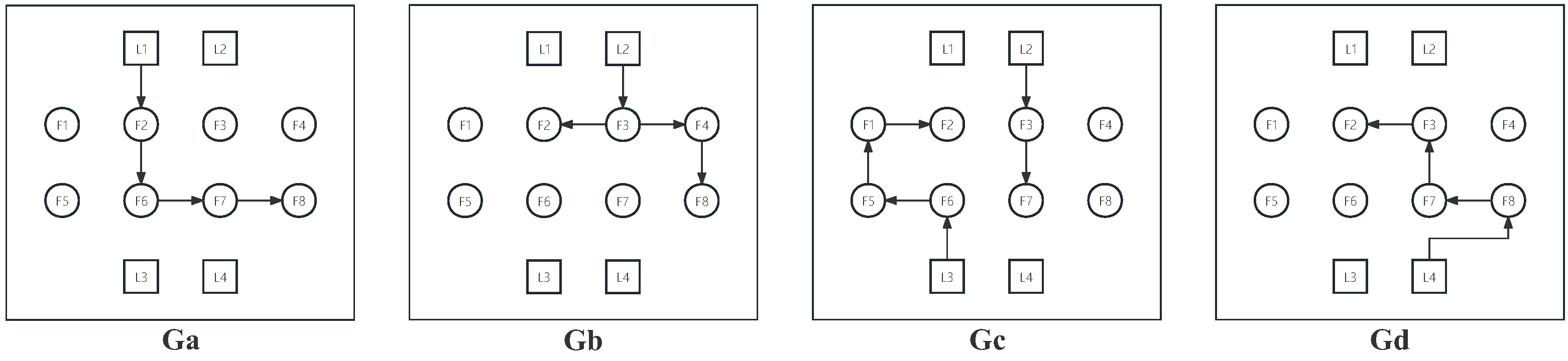
Consider an MAS consisting of 8 heterogeneous agents for $l=3$ and 4 leaders, where $i1,i2,i3,i4$ are second-order agents and $i5,i6,i7,i8$ are third-order agents. As is shown in Figure 1, the topologies of this MAS keep switching in the four graphs $Ga,Gb,Gc,andGd$ and their communication delays are, respectively, 0.5 s, 0.5 s, 1 s, 1 s, and, obviously, ${\tau }_{max}=1$ s, where Assumption 3 is satisfied with $M=1s$ and $\underline{M}=0.5s$. According to Assumption 2 and Equation (6), let $k_i=6.3,{\beta }_{i1}(t)\approx 0.1613$, ${\beta }_{i2}(t)\approx -0.1613$ for second-order agents $i1,i2,i3,i4$, and $k_i=2.7$${\beta }_{i1}(t)\approx 0.1826$, ${\beta }_{i2}(t)\approx 0.0070$, and ${\beta }_{i3}(t)\approx -0.1896$ for third-order agents $i5,i6,i7,i8$, and $q_{max}=0.025$. Then the parameters of control input are chosen as $p_i^{(2)}=0.32$, $p_i^{(3)}=0.56$, $b_i(t)=0.002$ if $b_i(t)>0$, and $a_{ij}(t)=0.005$ if $a_{ij}(t)>0$ for all $i,j,k,s$. The control input constraint set of each agent is considered as $U_i=\left\{(u_{i_1},u_{i_2})\right|((u_{i_1}^2+u_{i_2}^2\le {\underline{u}}_i^2)\cap (u_{i_1}\le 0))\cup ((u_{i_1}^2+u_{i_2}^2\le {\overline{u}}_i^2)\cap (u_{i_1}\ge 0))\}$ respectively, where ${\underline{u}}_i=0.04$ and ${\overline{u}}_i=0.05$. Obviously, Assumptions 1 and 2 are also satisfied.

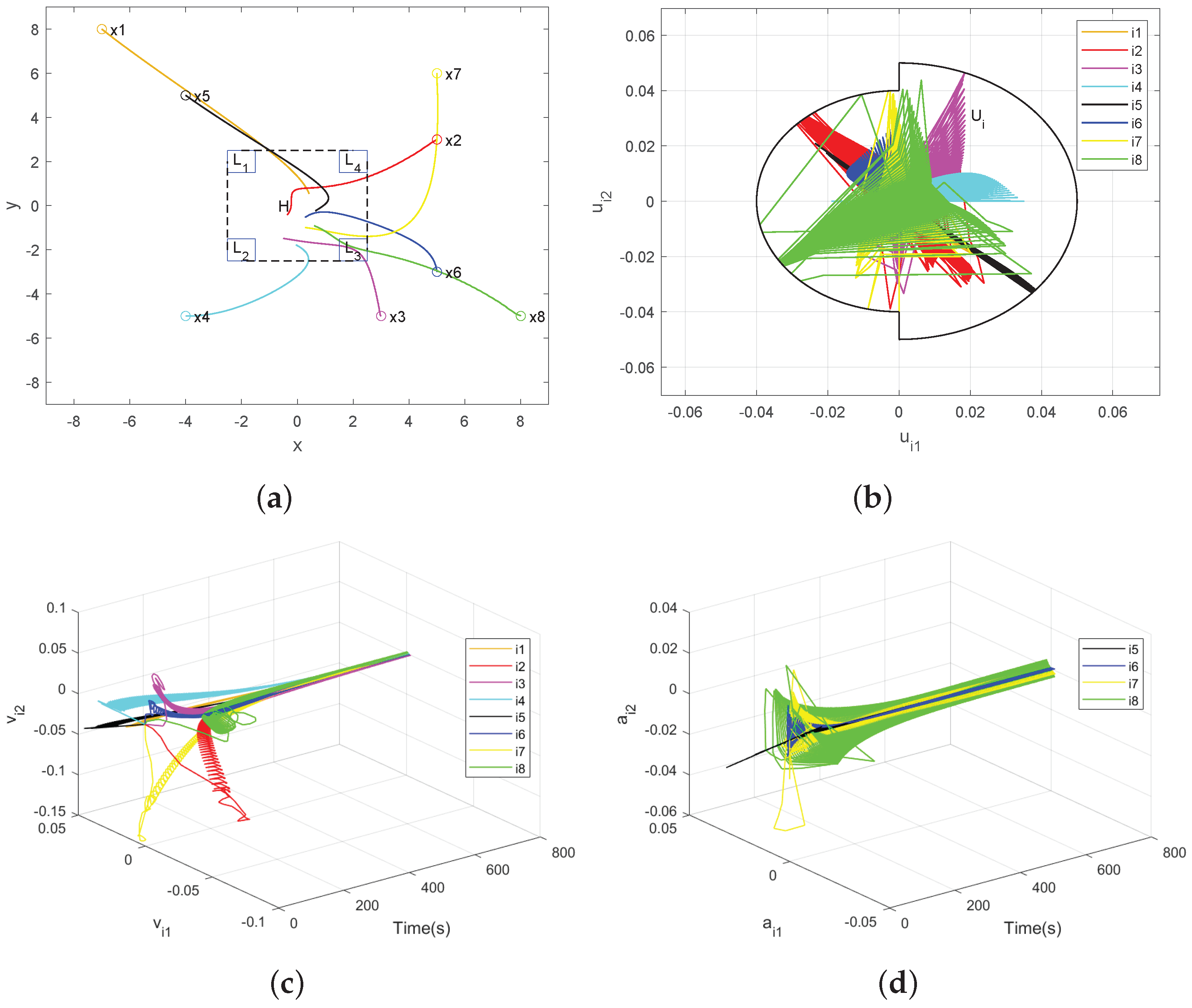
Figure 2a–d depict the simulation results of system (1) employing algorithm (3). Figure 2a shows the position trajectories, i.e., first-order states $x_i^{(1)}(t)$ of all agents. Figure 2b shows the control inputs $u_i(t)$ of all agents and they are constrained in the control input constraint set $U_i$. Figure 2c shows the second-order states $x_i^{(2)}(t)$ of all agents with time evolution, and Figure 2d shows the third-order states $x_i^{(3)}(t)$ of all agents with time evolution. Note that $i1,i2,i3,i4$ are second-order agents and, thus, no corresponding trajectories of third-order state appear in Figure 2d. It is evident that the presence of control input constraints, as shown in Figure 2b, imposes limitations on the control algorithm of each agent, preventing it from arbitrarily reaching desired values and desired convergence rate of the original unconstrained control input. As is shown in Figure 2a–d, each agent is eventually driven into the convex hull H spanned by the leaders $L1,L2,L3,L4$ over time, which aligns with the findings of Theorem 1.

5. Conclusions

This work studied containment control for high-order heterogeneous continuous-time MASs with input nonconvex constraints, bounded delays, and switching topologies. Firstly, we introduced a scaling factor for the constraint operator to obtain an equivalent unconstrained system model. Following equivalent model transformations, we analyzed the maximum distance from agents to the convex hull spanned by leaders using norm-based differentiation. It was shown that, within high-order heterogeneous continuous-time MASs subject to nonconvex control input constraints, the convergence of each agent into the convex hull spanned by leaders is guaranteed, provided that there exists at least one directed path from any leader to each agent within the union of communication graphs.

References

1. Ji, M.; Ferrari-Trecate, G.; Egerstedt, M.; Buffa, A. Containment control in mobile networks. IEEE Trans. Autom. Control 2008, 53, 1972–1975. [Google Scholar] [CrossRef]
2. Cheng, L.; Wang, Y.P.; Ren, W.; Hou, Z.G.; Tan, M. Containment control of multiagent systems with dynamic leaders based on a pin-type approach. IEEE Trans. Cybern. 2016, 46, 3004–3017. [Google Scholar] [CrossRef] [PubMed]
3. Li, J.Z.; Ren, W.; Xu, S.Y. Distributed containment control with multiple dynamic leaders for double-integrator dynamics using only position measurements. IEEE Trans. Autom. Control 2012, 57, 1553–1559. [Google Scholar] [CrossRef]
4. Liu, H.Y.; Xie, G.M.; Wang, L. Necessary and sufficient conditions for containment control of networked multi-agent systems. Automatica 2012, 48, 1415–1422. [Google Scholar] [CrossRef]
5. Meng, Z.Y.; Ren, W.; You, Z. Distributed finite-time attitude containment control for multiple rigid bodies. Automatica 2010, 46, 2092–2099. [Google Scholar] [CrossRef]
6. Liu, K.E.; Xie, G.M.; Wang, L. Containment control for second-order multi-agent systems with time-varying delays. Syst. Control Lett. 2014, 67, 24–31. [Google Scholar] [CrossRef]
7. Shen, J.; Lam, J. Containment control of multi-agent systems with unbounded communication delays. Int. J. Syst. Sci. 2016, 47, 2048–2057. [Google Scholar] [CrossRef]
8. Ajorlou, A.; Momeni, A.; Aghdam, A.G. A class of bounded distributed control strategies for connectivity preservation in multi-agent systems. IEEE Trans. Autom. Control 2010, 55, 2828–2833. [Google Scholar] [CrossRef]
9. Cao, Y.; Ren, W.; Egerstedt, M. Distributed containment control with multiple stationary or dynamic leaders in fixed andswitching directed networks. Automatica 2012, 48, 1586–1597. [Google Scholar] [CrossRef]
10. Notarstefano, G.; Egerstedt, M.; Haque, M. Containment in leader-follower networks with switching communication topologies. Automatica 2011, 47, 1035–1040. [Google Scholar] [CrossRef]
11. Lou, Y.C.; Hong, Y.G. Target containment control of multi-agent systems with random switching interconnection topologies. Automatica 2012, 48, 879–885. [Google Scholar] [CrossRef]
12. Shi, G.D.; Hong, Y.G.; Johansson, K.H. Connectivity and set tracking of multi-agent systems guided by multiple moving leaders. IEEE Trans. Autom. Control 2012, 57, 663–676. [Google Scholar]
13. Liu, H.; Xie, G.; Wang, L. Containment of linear multi-agent systems under general interaction topologies. Syst. Control Lett. 2012, 61, 528–534. [Google Scholar] [CrossRef]
14. Wen, G.; Zhao, Y.; Duan, Z. Containment of higher-order multi-leader multi-agent systems: A dynamic output approach. IEEE Trans. Autom. Control 2016, 61, 1135–1140. [Google Scholar] [CrossRef]
15. Lin, P.; Li, Z.; Jia, Y.; Sun, M. High-order multi-agent consensus with dynamically changing topologies and time-delays. IET Control Theory Appl. 2011, 5, 976–981. [Google Scholar] [CrossRef]
16. Dong, X.; Xi, J.; Lu, G.; Zhong, Y. Containment analysis and design for high-order linear time-invariant singular swarm systems with time delays. Int. J. Robust Nonlinear Control 2014, 24, 1189–1204. [Google Scholar] [CrossRef]
17. Wang, X.; Shi, L.; Shao, J. Containment control for high-order multi-agent systems with heterogeneous time delays. IET Control Theory Appl. 2018, 12, 1340–1348. [Google Scholar] [CrossRef]
18. Haghshenas, H.; Badamchizadeh, M.A.; Baradarannia, M. Containment control of heterogeneous linear multi-agent systems. Automatica 2015, 54, 210–216. [Google Scholar] [CrossRef]
19. Xiao, S.; Dong, J. Distributed Fault-Tolerant Containment Control for Linear Heterogeneous Multiagent Systems: A Hierarchical Design Approach. IEEE Trans. Cybern. 2020, 52, 971–981. [Google Scholar] [CrossRef] [PubMed]
20. Lui, D.G.; Petrillo, A.; Santini, S. An optimal distributed PID-like control for the output containment and leader-following of heterogeneous high-order multi-agent systems. Inf. Sci. 2020, 541, 166–184. [Google Scholar] [CrossRef]
21. Li, S.; Wang, F.; Er, M.J.; Yang, Z. Approximate output regulation of discrete-time stochastic multiagent systems subject to heterogeneous and unknown dynamics. IEEE Trans. Syst. Man Cybern. Syst. 2022, 52, 6373–6382. [Google Scholar] [CrossRef]
22. Lui, D.G.; Petrillo, A.; Santini, S. Distributed model reference adaptive containment control of heterogeneous multi-agent systems with unknown uncertainties and directed topologies. J. Frankl. Inst.-Eng. Appl. Math. 2021, 358, 737–756. [Google Scholar] [CrossRef]
23. Lin, P.; Ren, W.; Farrell, J.A. Distributed Continuous-Time Optimization: Nonuniform Gradient Gains, Finite-Time Convergence, and Convex Constraint Set. IEEE Trans. Autom. Control 2017, 62, 2239–2253. [Google Scholar] [CrossRef]
24. Lin, P.; Tian, Y.; Gui, G.; Yang, C. Cooperative control for multiple train systems: Self-adjusting zones, collision avoidance and constraints. Automatica 2022, 144, 110470. [Google Scholar] [CrossRef]
25. Lin, P.; Ren, W.; Yang, C.H.; Gui, W.H. Distributed continuous-time and discrete-time optimization with nonuniform unbounded convex constraint sets and nonuniform stepsizes. IEEE Trans. Autom. Control 2019, 64, 5148–5155. [Google Scholar] [CrossRef]
26. Lin, P.; Ren, W.; Yang, C.H.; Gui, W.H. Distributed optimization with nonconvex velocity constraints, nonuniform position constraints, and nonuniform stepsizes. IEEE Trans. Autom. Control 2019, 64, 2575–2582. [Google Scholar] [CrossRef]
27. Song, Q.; Liu, F.; Su, H.S.; Vasilakos, A.V. Semi-global and global containment control of multi-agent systems with second-order dynamics and input saturation. Int. J. Robust Nonlinear Control 2016, 26, 3460–3480. [Google Scholar] [CrossRef]
28. Wang, W.; Tong, S.C. Adaptive fuzzy containment control of nonlinear strict-feedback systems with full state constraints. IEEE Trans. Fuzzy Syst. 2019, 27, 2024–2038. [Google Scholar] [CrossRef]
29. Lin, P.; Ren, W.; Gao, H.J. Distributed velocity-constrained consensus of discrete-time multi-agent systems with nonconvex constraints, switching topologies, and delays. IEEE Trans. Autom. Control 2017, 62, 5788–5794. [Google Scholar] [CrossRef]
30. Lin, P.; Wang, Y.; Wang, D.; Wu, Z.-G. Constrained Containment Control for Multiagent Systems With Possible Empty Intersection of Position Constraints. IEEE Trans. Autom. Control 2024, 69, 1842–1849. [Google Scholar] [CrossRef]
31. Yang, C.; Duan, M.; Lin, P.; Ren, W.; Gui, W. Distributed containment control of continuous-time multiagent systems with nonconvex control input constraints. IEEE Trans. Ind. Electron. 2019, 66, 7927–7934. [Google Scholar] [CrossRef]
32. Xu, J.; Lin, P.; Cheng, L.; Dong, H. Containment control with input and velocity constraints. Automatica 2022, 142, 110417. [Google Scholar] [CrossRef]
33. Li, X.; Wang, L.; Zhang, Y. Distributed continuous-time containment control of heterogeneous multiagent systems with nonconvex control input constraints. Complexity 2022, 2022, 7081091. [Google Scholar] [CrossRef]
34. Li, X.; Li, C.; Yang, Y.; Mo, L. Consensus for heterogeneous multi-agent systems with nonconvex input constraints and nonuniform time delays. J. Frankl. Inst.-Eng. Appl. Math. 2020, 357, 3622–3635. [Google Scholar] [CrossRef]
35. Chris, G.; Royle, G. Algebraic Graph Theory; Springer: New York, NY, USA, 2001. [Google Scholar]
Figure 1. Four directed graphs.
Mathematics 13 00509 g001
Figure 2. The simulation results. (a) The 1st-order states x i ( 1 ) ( t ) of all agents. (b) The control inputs u i ( t ) of all agents. (c) The 2nd-order states x i ( 2 ) ( t ) of all agents with time evolution. (d) The 3rd-order states x i ( 3 ) ( t ) of all agents with time evolution.
Mathematics 13 00509 g002
Disclaimer/Publisher’s Note: The statements, opinions and data contained in all publications are solely those of the individual author(s) and contributor(s) and not of MDPI and/or the editor(s). MDPI and/or the editor(s) disclaim responsibility for any injury to people or property resulting from any ideas, methods, instructions or products referred to in the content.