Article

Sharp Estimates of Pochhammer’s Products

Faculty of Civil and Geodetic Engineering, University of Ljubljana, 1000 Ljubljana, Slovenia
Mathematics 2025, 13(3), 506; https://doi.org/10.3390/math13030506
Submission received: 1 December 2024 / Revised: 24 January 2025 / Accepted: 31 January 2025 / Published: 3 February 2025

Abstract

:
Sharp, asymptotic estimates of classical and generalized rising/falling Pochhammer’s products having positive arguments are presented on the basis of Stirling’s approximation formula for the Γ function.

1. Introduction

As a nontrivial example of where we can encounter the Pochhammer product (Leo August Pochhammer (1841–1920), German mathematician known for his work on special functions), let us take the sequence a n ( x ) , given recursively as a 0 ( x ) : = 1 and a n ( x ) : = x n k = 1 n a n k ( x ) , for n 1 and x 0 . The dynamics of this sequence strongly depend on the value of the parameter x and we would like to reveal it. It is easy to see that a n ( x ) satisfies the recursion a n + 1 ( x ) = x + n 1 + x a n ( x ) , for n 0 . Consequently, we have
a 1 ( p ) = x + 0 1 + 0 · a 0 ( x ) = x · 1 = x a 2 ( p ) = x + 1 1 + 1 · a 1 ( p ) = x + 1 2 · x = x ( x + 1 ) 2 a 3 ( p ) = x + 2 1 + 2 · x ( x + 1 ) 2 = x ( x + 1 ) ( x + 2 ) 2 · 3 .
Hence, using the total induction, we conclude with the following expression
a n ( x ) = x ( x + 1 ) ( x + 2 ) ( x + n 1 ) 1 · 2 · 3 n .
The product in the numerator of the fraction a n ( x ) is called the rising Pochhammer product of order n and basis x. We denote it by x ( n ) . The product in the denominator of a n ( x ) is called n-factorial and is denoted by n ! . Thus, n ! = 1 ( n ) and a n ( x ) = x ( n ) 1 ( n ) , for integers n 0 and any x, when we additionally define 0 ! = 1 ! = 1 , x ( 0 ) = 1 and x ( 1 ) = x .
For large n, the fraction a n ( x ) in (1) becomes complicated due to the many factors in its numerator and denominator. Thus, it is difficult to directly conclude the dynamics of the sequence a n ( x ) as a function of n and x. Therefore, it is imperative to simplify the sequence a n ( x ) or find its simple approximation to minimize the error of this approximation. Fortunately, Pochhammer’s product can be expressed with the famous gamma function, denoted by Γ , as x ( n ) = Γ ( x + n ) Γ ( x ) . In this way, we obtain the equality (considering the equality Γ ( 1 ) = 1 ) a n ( x ) = Γ ( x + n ) Γ ( x ) Γ ( n + 1 ) . Now, using the Stirling formula for approximating the gamma function [1] Sect. 9.5, we can provide the approximation of a n ( x ) . The obtained approximation allows us to investigate the dynamics of the sequence a n ( x ) as a function of x.
In our contribution, we will illustrate the usefulness of the derived approximation formulas for Pochhammer products using three examples of approximations of binomial coefficients. Namely, for integer n 1 , we will obtain the following approximations:
3 2 n ( 1 ) n 1128 1000 · n , 1 2 n ( 1 ) n 564 1000 · 1 n , 1 2 n ( 1 ) n + 1 282 1000 · 1 n n .
Pochhammer’s products or shifted factorials, falling (lower) and rising (upper), are often encountered in pure and applied mathematics as well as in several exact sciences. For example, the ordinary (Gaussian) hypergeometric function F 1 2 ( a , b ; c ; z ) is defined using rising Pochhammer products a ( n ) , b ( n ) and c ( n ) as
F 1 2 ( a , b ; c ; z ) : = n = 0 a ( n ) b ( n ) c ( n ) z n n ! .
The concept of Pochhammer’s product is constantly being generalized, see, e.g., [2].
Pochhammer’s products are found in combinatorics, number theory, probability, statistics, statistical physics, etc. These products are closely related to the famous Γ function, which is also accessible in a numerical sense, see, e.g., [1,3,4,5,6,7,8,9,10,11,12,13].
As we have already said, the classical rising Pochhammer’s product of the order n N = { 1 , 2 , 3 , } and the basis x C ,
x ( n ) : = j = 0 n 1 ( x + j ) = x · ( x + 1 ) · · ( x + n 1 ) ,
can be expressed, for x N , in terms of the Γ function as
x ( n ) = ( x + n 1 ) ! ( x 1 ) ! = Γ ( x + n ) Γ ( x ) .
There are only a few articles on approximating Pochhammer’s product. One of which is [7], where several approximations of the products in question are provided. In our paper, we would like to present sharper and more general results than those given in [7].
The final equation above suggests the most useful extension of the classical rising discrete-order Pochhammer’s factorial to a continuous-order Pochhammer’s factorial x ( p ) by setting the following definition.
Definition 1.
The rising Pochhammer’s factorial x ( p ) is defined as
x ( p ) : = Γ ( x + p ) Γ ( x ) , for x R + and a real p > x .
Obviously, x ( 0 ) = 1 and x ( 1 ) = x , for x R + .
Lemma 1.
For p , q , x R + , we have
x ( p ) = x ( q ) ( x + p ) ( q ) · ( x + q ) ( p ) .
Proof. 
Considering Definition 2, we have, for p , q , x R + ,
( x + q ) ( p ) = Γ ( x + q + p ) Γ ( x + q ) = Γ ( x + p + q ) Γ ( x + q ) = ( x + p ) ( q ) Γ ( x + p ) x ( q ) Γ ( x ) = ( x + p ) ( q ) x ( q ) x ( p ) .
The classical falling Pochhammer’s product of order n N = { 1 , 2 , 3 , } and basis x C ,
x ( n ) : = j = 0 n 1 ( x j ) = x · ( x 1 ) · · ( x n + 1 ) ,
can be expressed by the rising Pochhammer’s factorial, as
x ( n ) = x x n ( x n ) ( n ) ,
for an integer n and a real x satisfying x > n > 0 . Therefore, we extend the domain of the falling Pochhammer’s factorial to a continuous case setting
x ( p ) = x x p · ( x p ) ( p ) = x x p · Γ ( x ) Γ ( x p ) .
Moreover, as y Γ ( y ) = Γ ( y + 1 ) , for y > 0 , we set the next definition.
Definition 2.
The falling Pochhammer’s factorial x ( p ) is defined as
x ( p ) : = Γ ( x + 1 ) Γ ( x p + 1 ) = ( x p + 1 ) ( p ) , for x , p R + , such that x > p > 0 .
Obviously, x ( 0 ) = 1 and x ( 1 ) = x , for x R + .

2. Auxiliary Result (Approximation of Γ Function)

The Stirling approximation formula of order r 0 for the Γ function says that for x R + , we have [1] (Sect. 9.5)
Γ ( x ) = 2 π x · x e x · exp s r ( x ) + d r ( x ) ,
where
s 0 ( x ) 0 and s r ( x ) = i = 1 r B 2 i ( 2 i 1 ) ( 2 i ) x 2 i 1 for r 1 ,
and, for some Θ r ( x ) ( 0 , 1 ) ,
d r ( x ) = Θ r ( x ) · B 2 r + 2 2 r + 1 ( 2 r + 2 ) · x 2 r + 1 .
The numbers B 2 , B 4 , B 6 , …are known as the Bernoulli coefficients (the positive numbers ( 1 ) k + 1 B 2 k are called the Bernoulli numbers.). We have, for example,
B 2 = 1 6 , B 4 = B 8 = 1 30 , B 6 = 1 42 , B 10 = 5 66 , B 12 = 691 2730 , B 14 = 7 6 , B 16 = 3617 510 , B 18 = 43867 798 , B 20 = 174611 330 , B 22 = 854513 138 , B 24 = 236364091 2730 and B 26 = 8553103 6 ,
with the estimates 1 3 < B 12 < 1 4 , 8 < B 16 < 7 , 54 < B 18 < 55 , 530 < B 20 < 529 , 6192 < B 22 < 6193 , 86581 < B 24 < 86580 , 1.42 · 10 6 < B 26 < 1.43 · 10 6 .
As a consequence, we have for the (continuous) factorial function x ! : = Γ ( x + 1 ) = x Γ ( x ) the following expression (the Stirling factorial formula)
x ! = 2 π x x e x exp s r ( x ) + d r ( x ) ( x R + ) .

3. Approximations to Pochhammer’s Products

3.1. Approximation to Rising Product x ( p )

We are now able to prove our main result: a theorem on the asymptotic approximation of the generalized Pochhammer’s rising product.
Theorem 1.
For p , x R + and for integers m , r 0 , the equality
x ( p ) = P r ( x , m , p ) · exp δ r ( x , m , p )
holds, where, (considering σ 0 ( x , m , p ) = 0 , by definition)
P r ( x , m , p ) : = P * ( x , m , p ) · exp σ r ( x , m , p ) ,
P * ( x , m , p ) : = x ( m ) ( x + p ) ( m ) x + m + p x + m x + m 1 / 2 x + m + p e p ,
σ r ( x , m , p ) : = i = 1 r B 2 i ( 2 i 1 ) ( 2 i ) 1 ( x + m + p ) 2 i 1 1 ( x + m ) 2 i 1 ,
and, uniformly in p,
| δ r ( x , m , p ) | < δ ˜ r ( x , m ) : = | B 2 r + 2 | ( r + 1 ) ( 2 r + 1 ) ( x + m ) 2 r + 1 .
Proof. 
Using (2) and (6), we calculate
x ( p ) = 2 π x + p · x + p e x + p · exp s r ( x + p ) + d r ( x + p ) · 2 π x · x e x · exp s r ( x ) + d r ( x ) 1 = x + p x x 1 / 2 x + p e p exp s r ( x + p ) s r ( x ) · exp d r ( x + p ) d r ( x ) ,
where, according to (8), for p , x > 0 , we have
| d r ( x + p ) d r ( x ) | < 2 · | B 2 r + 2 | ( 2 r + 1 ) ( 2 r + 2 ) · x 2 r + 1 .
At small x the estimate (17) becomes useless. Therefore, using the identity (3), together with Formulas (16) and (17), replacing x with x + m , we find all relations of Theorem 1. □
Example 1.
For p , x > 0 , we have
P 0 ( x , 0 , p ) = P * ( x , 0 , p ) = x x + p 1 / 2 x x + p e p , δ ˜ 0 ( x , 1 ) < 1 6 ( x + 1 )
and
P 1 ( x , 1 , p ) = x x + p x + p + 1 x + 1 x + 1 / 2 x + p + 1 e p exp 1 12 1 x + p + 1 1 x + 1
with δ ˜ 1 ( x , 1 ) < 1 180 ( x + 1 ) 3 .
For x R + and any integer p 2 , we obviously have x p < x ( p ) < ( x + p 1 ) p . Moreover, setting m = 1 and r = 0 in Theorem 1, we obtain a more accurate estimate, given in the next corollary (which can be improved by increasing m).
Corollary 1.
For p , x R + , the following inequalities hold:
x ( p ) > A ( x , p ) : = x x + p x + p + 1 x + 1 x + 1 / 2 x + p + 1 e p exp 1 6 ( x + 1 )
x ( p ) < B ( x , p ) : = x x + p x + p + 1 x + 1 x + 1 / 2 x + p + 1 e p exp 1 6 ( x + 1 ) .
Figure 1 illustrates (all figures in this paper are produced using Mathematica [14]) relations (18) and (19) by plotting the graphs of the functions x A ( x , π ) and x B ( x , π ) , together with the graph (continuous line) of the function x P 2 ( x , 3 , π ) , which nearly coincides with the function x x ( π ) .
Remark 1.
In Formula (15), m and r are the parameters that affect the error term δ r * ( x , m , p ) . We stress that | B 2 r + 2 | becomes very large for large r. Indeed, according to [3] (23.1.15), we have
2 ( 2 n ) ! ( 2 π ) 2 n < | B 2 n | < 4 ( 2 n ) ! ( 2 π ) 2 n , for n N .
In addition, referring to (6) and (8), or using [15], we have the double inequality
2 π m m e m < m ! < 2 π m m e m exp 1 12 m , for m N .
Consequently,
4 π n n e π 2 n < | B 2 n | < 9 π n n e π 2 n , for n N .
Thus, considering (15), we find (considering the estimate r + 1 / ( 2 r + 1 ) < 1 / ( 2 r ) , for r > 0 )
δ ˜ r ( x , m ) < δ r * ( x , m ) : = 9 r + 1 e π ( 2 r + 1 ) r + 1 e π ( x + m ) 2 r + 1 ( m , r 0 , x > 0 )
< 1 r r + 1 e π ( x + m ) 2 r + 1 ( m 0 , r 1 , x > 0 ) .
Corollary 2.
For p , x R + and for integers m , r 1 , satisfying r 4 m 1 , the approximation x ( p ) P r ( x , m , p ) , given in Theorem 1, has the relative error
ρ r ( x , m , p ) : = x ( p ) P r ( x , m , p ) P r ( x , m , p ) ,
estimated as
| ρ r ( x , m , p ) | < 1 + 8 100 | δ r ( x , m , p ) | < 2 r r + 1 e π ( x + m ) 2 r + 1 .
Proof. 
According to Theorem 1, using Taylor’s formula, we obtain, for some ϑ ( 0 , 1 ) ,
| ρ r ( x , m , p ) | = P r e δ r P r P r = | e δ r 1 | = δ r + 1 2 e ϑ · δ r · δ r 2 | δ r | + e | δ r | 2 | δ r | · | δ r | .
Now, for integers m , r 1 , satisfying r 4 m 1 , and for x > 0 , we have 0 < r + 1 e π ( x + m ) < r + 1 8 ( x + m ) < 1 2 . Consequently, referring to (15) and (24), we estimate | δ r | < 1 r 1 2 2 r + 1 1 8 . Hence, considering (26), we obtain
| ρ r ( x , m , p ) | < | δ r | + e 1 / 8 2 · 1 8 · | δ r | < 1 + 8 100 | δ r | < 2 · | δ r | < 2 · | δ r * | .
The immediate consequence of Corollary 2 is the next corollary.
Corollary 3.
For p , x R + and for integers m , r 1 , satisfying r 4 m 1 , the inequalities
x ( p ) > 1 2 r r + 1 e π ( x + m ) 2 r + 1 P r ( x , m , p )
x ( p ) < 1 + 2 r r + 1 e π ( x + m ) 2 r + 1 P r ( x , m , p )
hold.
Example 2.
Setting r = 1 and r = 7 in Corollary 3 we obtain the following double inequalities:
1 1 50 ( x + m ) 3 P 1 ( x , m , p ) < x ( p ) < 1 + 1 50 ( x + m ) 3 P 1 ( x , m , p ) ,
true for p , x R + and m 1 , and
1 1 4 ( x + m ) 15 P 7 ( x , m , p ) < x ( p ) < 1 + 1 4 ( x + m ) 15 P 7 ( x , m , p ) ,
valid for p , x R + and m 2 .
The inequalities in (29) are illustrated in Figure 2, where the dashed line represents the graph of the function x P 0 ( x , 1 , π ) and the continuous line, compressed between the nearly coinciding graphs of the functions x 1 1 50 ( x + 1 ) 3 P 1 ( x , 1 , π ) , represents the graph of the function x x ( π ) .

3.2. Dynamics of the Sequence r δ r ( x , m , p )

We are interested in how the sequence r δ r ( x , m , p ) varies. Indeed, thanks to Theorem 1, for p , x R + and integers m , r , r 0 , we have
P * ( x , m , p ) · exp σ r ( x , m , p ) + δ r ( x , m , p ) = x ( p ) = P * ( x , m , p ) · exp σ r ( x , m , p ) + δ r ( x , m , p ) .
Therefore, for integers 0 r < r and m 0 , for real p , x > 0 , and for the difference D r , r ( x , m , p ) ,
D r , r ( x , m , p ) : = σ r ( x , m , p ) σ r ( x , m , p ) = i = r + 1 r B 2 i ( 2 i 1 ) ( 2 i ) 1 ( x + m + p ) 2 i 1 1 ( x + m ) 2 i 1 ,
using (15), we estimate
δ r ( x , m , p ) > D r , r ( x , m , p ) δ ˜ r ( x , m ) δ r ( x , m , p ) < D r , r ( x , m , p ) + δ ˜ r ( x , m ) .
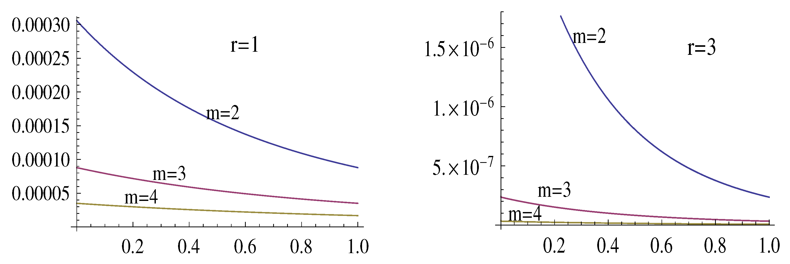
The inequalities (32) can be used to estimate the error δ r ( x , m , p ) by using the appropriate r > r , which specifies a negligibly small δ ˜ r ( x , m ) < δ r * ( x , m ) (see (23)) and, thus, provides a useful estimate for δ r ( x , m , p ) . Figure 3 and Figure 4 illustrate the estimate (32), for r { 0 , 1 , 2 , 3 } , by showing the graphs of the functions (with δ ˜ 5 ( x , 4 ) < 1 5 5 + 1 8 ( 0 + 4 ) 2 · 5 + 1 < 5 × 10 9 ) x D r , 5 ( x , 4 , π ) δ ˜ 5 ( x , 4 ) and x D r , 5 ( x , 4 , π ) + δ ˜ 5 ( x , 4 ) , cramming the graphs of the functions x δ r ( x , 4 , π ) .
Remark 2
(open problem). Figure 3, Figure 4, Figure 5 and Figure 6 suggest the hypotheses that ( 1 ) r + 1 δ r ( x , m , p ) > 0 , for all allowed values of all arguments.

3.3. Approximation to Continuous Factorial Function

For p N , the quantity p ! = k = 1 p k = 1 ( p ) is called p-factorial. The discrete factorial function p p ! is extended continuously, for real p > 1 , as p ! : = 1 ( p ) . Immediately, from Theorem 1, we read the next corollary, which presents a formula for p ! that does not contain the constant π , compared with Formula (10).
Corollary 4
(approximation of the continuous factorial function). For p R + and integers m , r 0 , we have (taking into account the definition i = 1 0 x i = : 0 .)
p ! = m ! ( p + 1 ) ( m ) m + p + 1 m + 1 m + 1 / 2 m + p + 1 e p · exp i = 1 r B 2 i ( 2 i 1 ) ( 2 i ) 1 ( m + p + 1 ) 2 i 1 1 ( m + 1 ) 2 i 1 + ϑ · | B 2 r + 2 | ( r + 1 ) ( 2 r + 1 ) ( p + m ) 2 r + 1 ,
for some ϑ = ϑ ( m , p , r ) from the interval ( 1 , 1 ) .

3.4. Approximation to Falling Product x ( p )

Using Definition 2 and Theorem 1, we obtain the approximation of the generalized Pochhammer’s falling product, presented in the next theorem.
Theorem 2.
For real x , p , satisfying x > p > 0 and for integers m , r 0 , we have the equality
x ( p ) = Q r ( x , m , p ) · exp Δ r ( x , m , p ) ,
where Q r ( x , m , p ) = P r ( x p + 1 , m , p ) , that is
Q r ( x , m , p ) : = ( x p + 1 ) ( m ) ( x + 1 ) ( m ) x + 1 + m x p + 1 + m x p + m + 1 / 2 · x + 1 + m e p exp σ r ( x p + 1 , m , p ) ,
with σ r ( x , m , p ) defined in (14), and
| Δ r ( x , m , p ) | < Δ r * ( x , m , p ) : = | B 2 r + 2 | ( r + 1 ) ( 2 r + 1 ) ( x p + 1 + m ) 2 r + 1 .
Remark 3.
For x R + and any integer p, satisfying 2 p < x , we obviously have ( x p + 1 ) p < x ( p ) < x p . In addition, using the inequality 1 + p t t < e p , true for t > | p | , from (35), we obtain
Q r ( x , m , p ) < x x p · ( x p ) ( m ) x ( m ) 1 + p x + m p x + m p x + m p x + m p p · x + m x + m p 1 / 2 x + m p p · e p < x x p · ( x p ) ( m ) x ( m ) · e p · ( x + m ) p · 1 · e p .
Thus, for all integers m 0 and x , p R + , such that p < x , we have a rough estimate (interesting for a larger m)
Q r ( x , m , p ) < x x p · ( x p ) ( m ) x ( m ) · ( x + m ) p .
Using Definition 2 and Corollary 3, we read the next result.
Corollary 5.
For real p , x satisfying x > p > 0 and for integers m , r 1 , such that r 4 m 1 , the inequalities
x ( p ) > 1 2 r r + 1 e π ( x p + 1 + m ) 2 r + 1 Q r ( x , m , p )
and
x ( p ) < 1 + 2 r r + 1 e π ( x p + 1 + m ) 2 r + 1 Q r ( x , m , p )
hold.
Thanks to Corollary 5, the approximation x ( p ) Q r ( x , m , p ) has a relative error ε r ( x , m , p ) : = x ( p ) Q r ( x , m , p ) / Q r ( x , m , p ) estimated as
| ε r ( x , m , p ) | < 2 r r + 1 e π ( x p + 1 + m ) 2 r + 1 ,
true for x , p , m , r that meet all conditions given in Corollary 5.

4. Examples of Using Approximation Formulas

According to (4), the binomial coefficient “x over n”,
x n : = k = 0 n 1 ( x k ) n ! = x ( n ) 1 ( n ) ( x R , n N ) ,
can be expressed using the upper Pochhammer’s product ac cording to the following Proposition.
Proposition 1.
For every real x and any integer n 3 , we have (for x > 0 , the floor symbol x means the integer part of x.)
x n n ! = ( 1 ) n | x | ( n ) ( x 0 ) , ( 1 ) n 1 x x x ( x + 1 ) x + 1 x ( n 1 x ) ( 0 < x < n ) , x n + 1 ( n ) ( x n ) .
Proof. 
The first and last cases are obvious. Relating to the second one, for 0 < x < n , we have (considering the equality k = m n y k = 1 , for m > n , true by definition)
k = 0 n 1 ( x k ) = k = 0 x ( x k ) k = x + 1 n 1 ( x k ) = j = 0 x ( x x + j ) · ( 1 ) n 1 x k = x + 1 n 1 ( k x ) = ( 1 ) n 1 x · x x ( x + 1 ) · x + 1 x n 1 x .
Thanks to Proposition 1, Theorem 1, and (10), we present the following three examples.
Example 3.
Using m = 4 and r = 1 in Theorem 1 and in (10), we obtain, for some ϑ ( 0 , 1 ) and Θ ( 1 , 1 ) , the following relations:
3 2 n = ( 1 ) n 3 2 ( n ) n ! = ( 1 ) n 3 2 ( 4 ) 3 2 + n ( 4 ) 3 2 + 4 + n 3 2 + 4 3 2 + 4 1 2 3 2 + 4 + n e n · exp 1 6 1 · 2 1 3 2 + 4 + n 1 3 2 + 4 + Θ · ( 1 30 2 · 3 ( 3 2 + 4 ) 3 · 1 2 π n e n n exp 1 6 1 · 2 · n ϑ · ( 1 30 ) 3 · 4 · n 3 .
Thus, for every n N and some ϑ ( 0 , 1 ) and Θ ( 1 , 1 ) , we have
3 2 n = ( 1 ) n · 3 · 5 · 7 · 9 · ( 11 + 2 n ) 5 ( 3 + 2 n ) ( 5 + 2 n ) ( 7 + 2 n ) ( 9 + 2 n ) · 11 5 · 2 π n 1 + 11 / 2 n n · exp 1 12 2 11 + n 2 11 1 n + ϑ 360 n 3 Θ 180 ( 3 2 + 4 ) 3 .
Hence,
3 2 n b 1 ( n ) : = ( 1 ) n · 3 · 5 · 7 · 9 2 n 11 5 π · exp 11 2 2 12 · 11 ( 1 ) n 1128 1000 n , for an integer n 1 .
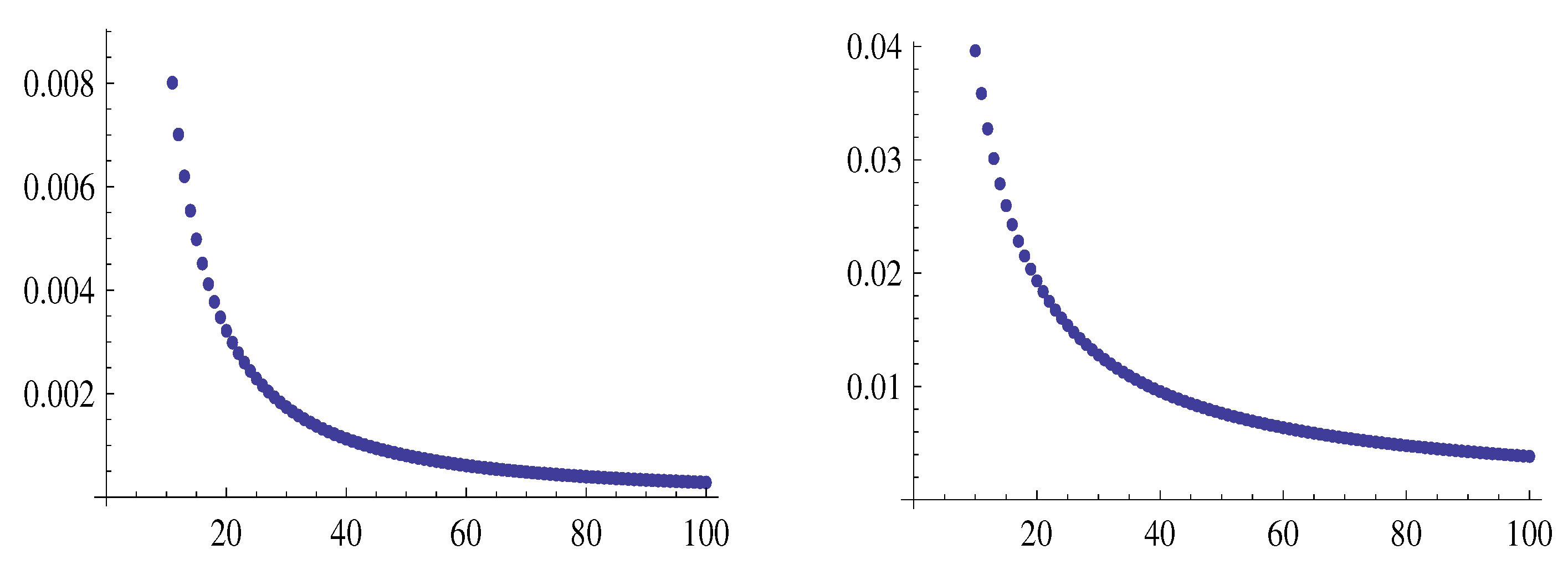
Figure 7 shows the graphs of the sequences n | 3 2 n | and n | 3 2 n b 1 ( n ) | | b 1 ( n ) | , left and right, respectively.
Example 4.
Setting m = 3 and r = 2 in Theorem 1 and (10), we obtain, for some ϑ ( 0 , 1 ) and Θ ( 1 , 1 ) , the next equalities:
1 2 n = ( 1 ) n 1 2 ( n ) n ! ̲ ̲ = ( 1 ) n 1 2 ( 3 ) 1 2 + n ( 3 ) 1 2 + 3 + n 1 2 + 3 1 2 + 3 1 2 1 2 + 3 + n e n · exp 1 6 1 · 2 1 1 2 + 3 + n 1 1 2 + 3 + 1 30 3 · 4 1 ( 1 2 + 3 + n ) 3 1 ( 1 2 + 3 ) 3 + Θ · 1 42 5 · 6 ( 1 2 + 3 ) 5 · 1 2 π n e n n exp 1 6 1 · 2 · n 1 30 3 · 4 · n 3 ϑ · 1 42 5 · 6 · n 5 .
Therefore, for any n N , using some ϑ ( 0 , 1 ) and Θ ( 1 , 1 ) , we find
1 2 n = ( 1 ) n · 3 · 5 · ( 7 + 2 n ) 3 ( 1 + 2 n ) ( 3 + 2 n ) ( 5 + 2 n ) · 7 3 · 2 π n 1 + 7 / 2 n n · exp ( 1 12 2 7 + n 2 7 1 n + 1 360 1 n 3 1 ( 1 2 + 3 + n ) 3 + 1 ( 1 2 + 3 ) 3 + Θ 1260 ( 1 2 + 3 ) 5 ϑ 1260 n 5 ) .
Hence,
1 2 n b 2 ( n ) : = ( 1 ) n 3 · 5 7 3 2 π exp 7 2 1 42 · 1 n ( 1 ) n 564 1000 n , for an integer n 1 .
Figure 8 shows the graphs of the sequences n | 1 2 n | and n | 1 2 n b 2 ( n ) | | b 2 ( n ) | , left and right, respectively.
Example 5.
Using m = 3 and r = 2 in Theorem 1 and in (10), and considering Example 4, we have (using the identity x ( n ) = ( x + n 1 ) x ( n 1 ) )
1 2 n = 1 n ! · ( 1 ) n 1 1 2 ( 1 ) 1 2 ( n 1 ) = 1 2 ( n 1 2 ) · ( 1 ) n 1 2 ( n ) n ! ̲ ̲ = 1 2 ( n 1 2 ) · ( 1 ) n · 3 · 5 · ( 7 + 2 n ) 3 ( 1 + 2 n ) ( 3 + 2 n ) ( 5 + 2 n ) · 7 3 · 2 π n 1 + 7 / 2 n n · exp ( 1 12 2 7 + n 2 7 1 n + 1 360 1 n 3 1 ( 1 2 + 3 + n ) 3 + 1 ( 1 2 + 3 ) 3 + Θ 1260 ( 1 2 + 3 ) 5 ϑ 1260 n 5 ) ,
for some ϑ ( 0 , 1 ) and Θ ( 1 , 1 ) . Thus, for every n N , there exists some ϑ ( 0 , 1 ) and some Θ ( 1 , 1 ) , such that
1 2 n = ( 1 ) n + 1 15 · ( 7 + 2 n ) 3 ( 2 n 1 ) · ( 1 + 2 n ) ( 3 + 2 n ) ( 5 + 2 n ) · 7 3 · 2 π n 1 + 7 / 2 n n · exp ( 1 12 2 7 + n 2 7 1 n + 1 360 1 n 3 1 ( 1 2 + 3 + n ) 3 + 1 ( 1 2 + 3 ) 3 + Θ 1260 ( 1 2 + 3 ) 5 ϑ 1260 n 5 ) .
Consequently,
1 2 n b 3 ( n ) : = ( 1 ) n + 1 15 7 3 2 π exp 7 2 1 42 · 1 ( 2 n 1 ) n ( 1 ) n + 1 282 1000 n n , for an integer n 1 .
Figure 9 shows the graphs of the sequences n | 1 2 n | and n | 1 2 n b 3 ( n ) | | b 3 ( n ) | , left and right, respectively.
Remark 4.
More about binomial coefficients can be found in [16].

5. Conclusions

In this contribution, we provided the approximations to generalized (classical) rising and falling Pochhammer’s products: x ( p ) P r ( x , m , p ) and x ( p ) Q r ( x , m , p ) . The relative errors ρ r ( x , m , p ) : = x ( p ) P r ( x , m , p ) / P r ( x , m , p ) and ε r ( x , m , p ) : = x ( p ) Q r ( x , m , p ) / Q r ( x , m , p ) of these approximations were estimated as
| ρ r ( x , m , p ) | < 2 r r + 1 e π ( x + m ) 2 r + 1 ( p , x > 0 , m , r 1 , r 4 m 1 ) , | ε r ( x , m , p ) | < 2 r r + 1 e π ( x p + 1 + m ) 2 r + 1 ( x > p > 0 , m , r 1 , r 4 m 1 ) .
In this paper, we also illustrated the usefulness of the derived approximation formulas with three examples of approximations for binomial coefficients.

Funding

This research received no external funding.

Data Availability Statement

Data are contained within the article.

Conflicts of Interest

The author declares no conflict of interest.

References

  1. Graham, R.L.; Knuth, D.E.; Patashnik, O. Concrete Mathematics: A Foundation for Computer Science; Addison-Wesley: Reading, MA, USA, 1994. [Google Scholar]
  2. Srivastava, R. Some Generalizations of Pochhammer’s Symbol and their Associated Families of Hypergeometric Functions and Hypergeometric Polynomials. Appl. Math. Inf. Sci. 2013, 7, 2195–2206. [Google Scholar] [CrossRef]
  3. Abramowitz, M.; Stegun, I.A. Handbook of Mathematical Functions, 9th ed.; Dover Publications: New York, NY, USA, 1974. [Google Scholar]
  4. Alzer, H. Sharp upper and lower bounds for the Gamma function. Proc. R. Soc. Edinb. Sect. Math. 2009, 139, 709–718. [Google Scholar] [CrossRef]
  5. Chen, C.P. A more accurate approximation for the gamma function. J. Number Theory 2016, 164, 417–428. [Google Scholar] [CrossRef]
  6. Henrici, P. Applied and Computational Complex Analysis; Wiley: New York, NY, USA, 1977; Volume 2, Section 8.4. [Google Scholar]
  7. Lampret, V. Approximating real Pochhammer products: A comparison with powers. Open Math. (Cent. Eur. J. Math.) 2009, 7, 493–505. [Google Scholar] [CrossRef]
  8. Mahmoud, M.; Alsulami, S.M.; Almarashi, S. On Some Bounds for the Gamma Function. Symmetry 2023, 15, 937. [Google Scholar] [CrossRef]
  9. Olver, F.W.J. Asymptotics and Special Functions; A.K. Peters Ltd. (AKP Classics): Wellesley, MA, USA, 1997. [Google Scholar]
  10. Whittaker, E.T.; Watson, G.N. A Course of Modern Analysis, 4th ed.; Cambridge University Press: Cambridge, UK, 1950. [Google Scholar]
  11. Yang, Z.H.; Chu, Y.M. Asymptotic formulas for gamma function with applications. Appl. Math. Comput. 2015, 270, 665–680. [Google Scholar] [CrossRef]
  12. Yang, Z.H.; Tian, J. Two asymptotic expansions for Gamma function developed by Windschitl’s formula. Open Math. 2017, 16, 1048–1060. [Google Scholar] [CrossRef]
  13. Yang, Z.H.; Tian, J.F. An accurate approximation formula for gamma function. J. Inequal. Appl. 2018, 2018, 56. [Google Scholar] [CrossRef] [PubMed]
  14. Wolfram, S. Mathematica; Version 7.0; Wolfram Research, Inc.: Champaign, IL, USA, 2008. [Google Scholar]
  15. Robbins, H. A Remark on Stirling Formula. Am. Math. Mon. 1955, 62, 26–29. [Google Scholar]
  16. Lampret, V. Accurate approximations of classical and generalized binomial coefficients. Comput. Appl. Math. 2024, 43, 341. [Google Scholar] [CrossRef]
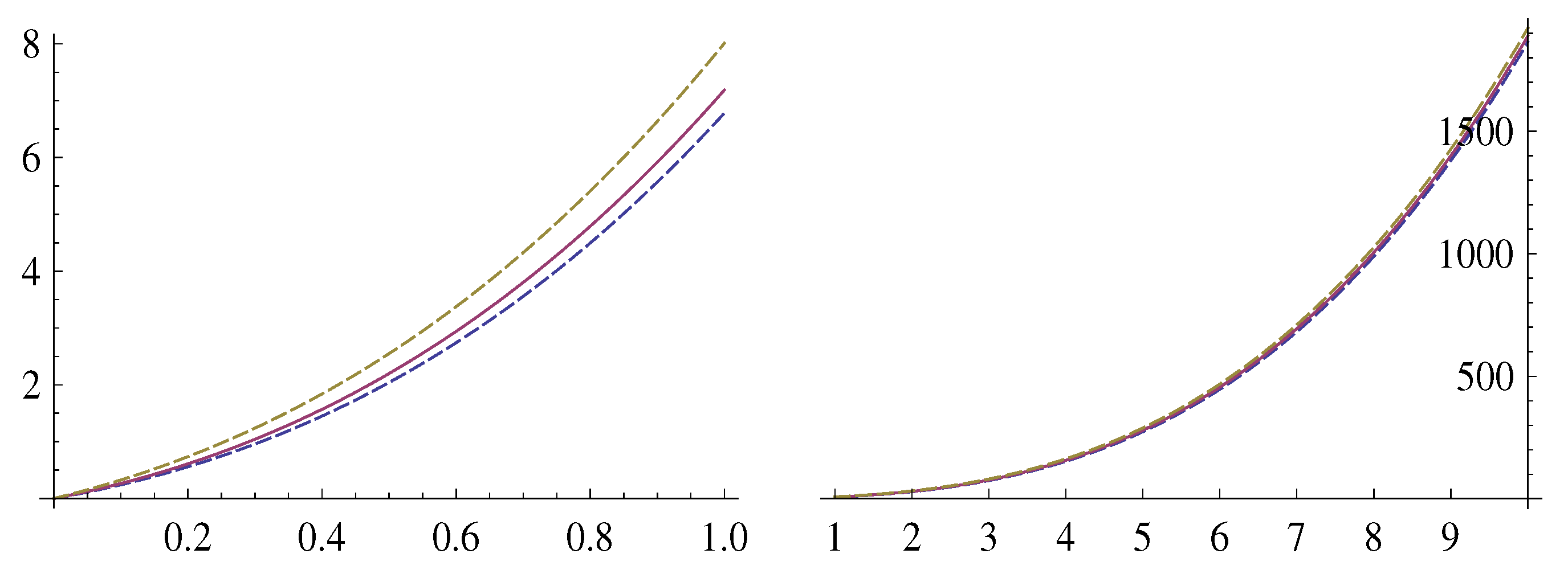
Figure 1. The graphs of the functions x A ( x , π ) , x B ( x , π ) and x x ( π ) from Corollary 1.
Mathematics 13 00506 g001
Figure 2. The graph of the function x P 0 ( x , 1 , π ) (dashed line) and the practically coinciding graphs of the functions x 1 1 50 ( x + 1 ) 3 P 1 ( x , 1 , π ) (continuous line).
Mathematics 13 00506 g002
Figure 3. The graphs of the functions x δ r ( x , 4 , π ) .
Mathematics 13 00506 g003
Figure 4. The graphs of the functions x D r , 5 ( x , 4 , π ) δ ˜ 5 ( x , 4 ) δ r ( x , 4 , π ) .
Mathematics 13 00506 g004
Figure 5. The graphs of the functions x δ r ( x , m , π ) .
Mathematics 13 00506 g005
Figure 6. The graphs of the functions x δ r ( x , m , π ) .
Mathematics 13 00506 g006
Figure 7. The graphs of the sequences | 3 2 n | and | 3 2 n b 1 ( n ) | / | b 1 ( n ) | , left and right respectively.
Mathematics 13 00506 g007
Figure 8. The graphs of the sequences | 1 2 n | and | 1 2 n b 2 ( n ) | / | b 2 ( n ) | , left and right, respectively.
Mathematics 13 00506 g008
Figure 9. The graphs of the sequences | 1 2 n | and | 1 2 n b 3 ( n ) | / | b 3 ( n ) | , left and right respectively.
Mathematics 13 00506 g009
Disclaimer/Publisher’s Note: The statements, opinions and data contained in all publications are solely those of the individual author(s) and contributor(s) and not of MDPI and/or the editor(s). MDPI and/or the editor(s) disclaim responsibility for any injury to people or property resulting from any ideas, methods, instructions or products referred to in the content.