A Model-Based Heuristic for Packing Soft Rotated Rectangles in an Optimized Convex Container with Prohibited Zones

Abstract

Packing soft rectangular objects in an optimized convex container is considered. Each soft rectangle can be freely translated and rotated, has a fixed area, and its dimensions can vary in certain limits. The convex container may have prohibited zones where allocation of the objects is not allowed. The soft rectangles must be arranged completely inside the container; mutual intersection and overlapping with prohibited zones is not allowed. The objective is to minimize a certain metric characteristic of the container. The corresponding nonlinear mathematical problem is formulated using the phi-function technique to present non-overlapping and containment conditions. A model-based heuristic is proposed to find reasonable solutions to the problem. Numerical results are provided for triangular, circular, and scaled polygonal containers to validate the model and demonstrate the proposed approach’s efficiency.

1. Introduction

The soft rectangle packing problem deals with soft rectangular objects whose areas are fixed, while their dimensions (width and height) can be adjusted in certain limits. Problems of optimized packing of soft rectangular objects arise, e.g., in land design/allocation [1,2,3] and floorplanning of soft modules [4,5,6], parallel computing [7] and VLSI computer chip design [8,9,10,11], facility layout [12], and designing a multi-channel conduit [13,14].

In the applications mentioned above, soft rectangles must be packed in a rectangular container subject to non-overlapping and containment conditions. That is, the objects must be arranged without mutual overlapping and completely inside the container. For a fixed number of rectangles, the objective is to optimize the size of the corresponding rectangular container, while for the fixed container, the objective is either to maximize the number of packed soft rectangles or to optimize an indicator associated with the perimeters of the objects. For the case of the fixed container, additional conditions, such as guillotine constraints, can be considered [2,3].

For packing soft rectangles in a fixed rectangular container there are plenty of theoretical estimations for the correspondence between parameters of the container, and soft rectangles to fit into the container [15,16,17,18,19].

If soft rectangles are packed in a rectangular container, then there exists an optimal layout where the objects are aligned along the sides of the container. This observation is used in many numerical algorithms for the problem. A simulated annealing framework based on the sequence pair representation of the placement topology is proposed in [1] for rectangular soft modules floorplanning. Here the sequence corresponds to a permutation of a given module set. Partitioning a given rectangular region into a fixed number of soft rectangles of known areas using guillotine cuts is considered in [2,3]. The objective is to minimize either the largest perimeter or the maximum aspect ratio of the rectangles. Corresponding mixed integer programming formulations are proposed. A binary search-based solution approach is used in [2], while metaheuristics (Variable Neighborhood Search and Tabu Search) are implemented in [3]. An alternative solution approach to the partitioning problem is proposed in [5], where a heuristic based on iteratively merging two rectangles into a composite rectangle is used. Additional adjacency relations are considered in [6] for the floorplanning problem, and a linear programming-based approach is used to construct a feasible floorplan. In [7] the rectangular region partitioning problem motivated by matrix multiplication on heterogeneous platforms is approached by a column-based heuristic. Packing a collection of hard, soft, and fixed-position rectangles (prohibited zones) in a minimum square rectangular container is considered in [8] and is approached by a heuristic based on a sequence pair placement topology. The sequence pair modeling approach is also used in [9], combined with simulated annealing and Lagrangian relaxation. In [10] a preliminary floorplan is constructed, and then the shapes of the flexible modules are adjusted in a best-fit way to fill up the unused area of a preliminary floorplan while keeping the relative positions between the modules unchanged. In this approach the adjusted modules are allowed to be rectilinear (L-shapes, T-shapes, etc.), and Lagrangian relaxation is used to solve the corresponding adjustment problem. A quick heuristic is proposed in [11] to determine the aspect ratio of each soft module subject to keeping a given relative position between modules. The proposed method is implemented with Simulated Annealing and consists of two main steps: selection of a set of soft modules to adjust the aspect ratio and decision on the aspect ratio of elements in the set. In [12] a specific two-dimensional rectangle packing area minimization problem with a central rectangle is considered. In this problem there exists at least one specific item (central rectangle) which must be placed near the center of the final layout. A heuristic solution approach is proposed based on three strategies: monitoring the aspect ratio, decreasing computational complexity, and filling the marginal inner space. The design of multi-channel conduit is considered in [13] to find a topology that consists of several channels with a given cross-section area using a minimum amount of sheet metal and, at the same time, maximizing its stiffness. Using a regular quadratic grid, rectilinear channels are represented by combinations of squares, and a corresponding large-scale linear mixed-integer programming problem is solved by cut generation. Another problem motivated by multi-channel conduit design is considered in [14] and consists in the arrangement of rectangles with given areas that minimizes the total length of all inner and outer border lines. A nonlinear mixed integer formulation is presented, and several approximation algorithms are provided along with an estimation of the proximity indicators.

In this paper, packing soft rectangles in an optimized convex (not necessarily rectangular) container is considered. For the rectangular container in the optimal arrangement, all soft rectangles are allocated such that their sides are parallel to the sides of the container. However, if the container is not rectangular, e.g., circular or triangular, rotation of the objects is essential to obtain the optimal arrangement. Moreover, in many applications, e.g., in land design or floor planning, the area for allocation of the soft rectangles (container) may have different zones prohibited for allocations. These can be, e.g., lakes or forests in the case of land design, columns or elevators in the case of floor planning. The presence of the prohibited zones is another reason for the arising rotated soft rectangles in the optimal arrangement. To the best of our knowledge, packing soft rectangles with free rotations allowed in convex containers has never been considered before.

The main contributions of this paper are:

1.

The problem of optimized packing of soft, rotated rectangles in a convex, optimized container with prohibited zones (OPSR) is formulated.

2.

Non-overlapping and containment conditions considering prohibited zones are presented using the phi-functions technique [20,21].

3.

A nonlinear mathematical model corresponding to the OPSR problem is formulated for optimized triangular, rectangular, circular, and scaled convex containers and prohibited zones.

4.

A model-based heuristic is proposed to obtain reasonable solutions for the corresponding large-scale nonconvex optimization problem.

5.

Numerical experiments are provided to demonstrate the efficiency of the proposed solution approach.

The rest of the paper is organized as follows. Section 2 presents the problem formulation. A mathematical model is described in Section 3. Section 4 introduces a solution approach, while numerical experiments are reported in Section 5. The last section, Section 6, provides conclusions and directions for future research. The proof of the proposition from Section 2 is given in Appendix A, while the concept of phi-functions is defined in Appendix B.

2. Problem Formulation

The following geometric objects are used in the problem formulation.

Containers. Let $\Omega \left(L\right)$ be a convex domain/container given in the fixed coordinate system $OXY$, where L is a vector of unknown/variable parameters of $\Omega$.

Within this study the following shapes are considered for the containers:

• rectangular container with variable dimensions l and h, $L=\{l,h\}$

  $$\Omega \left(l,h\right)=\{(x,y)\in {\mathbb{R}}^2\left|min\left\{{\omega }_1(x,y),{\omega }_2(x,y),{\omega }_3(x,y),{\omega }_4(x,y)\right\}\right.\ge 0\},$$

  where

  $${\omega }_1(x,y)=x, {\omega }_2(x,y)=-x+l, {\omega }_3(x,y)=y, {\omega }_4(x,y)=-y+h;$$
• Circular container with variable radius r, $L=\left\{r\right\}$:

  $$\Omega \left(r\right)=\{(x,y)\in {\mathbb{R}}^2\left|\phi (x,y)=-x^2-y^2+r^2\ge 0\right.\};$$
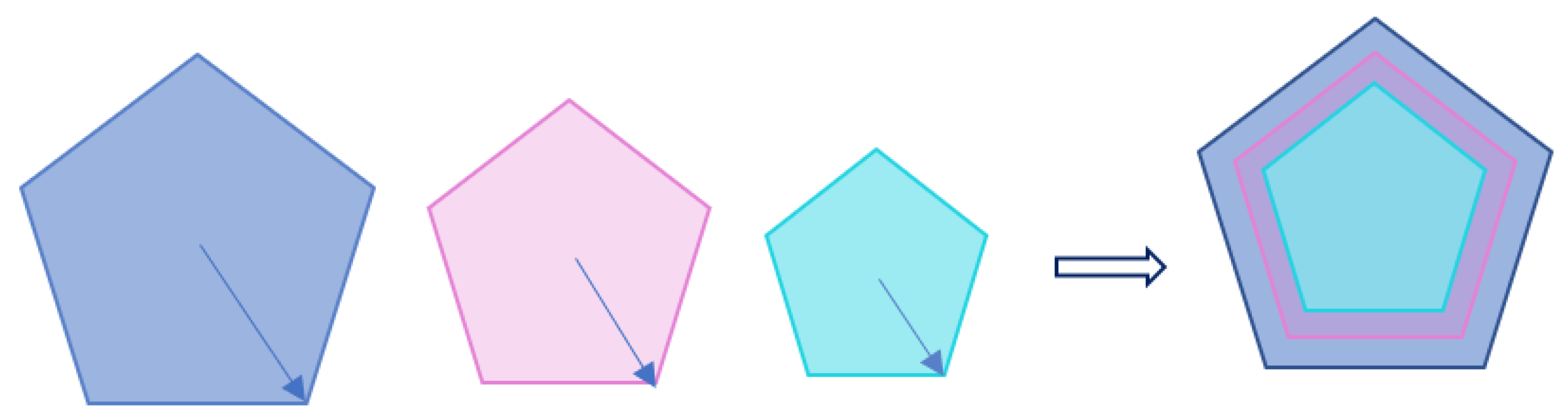
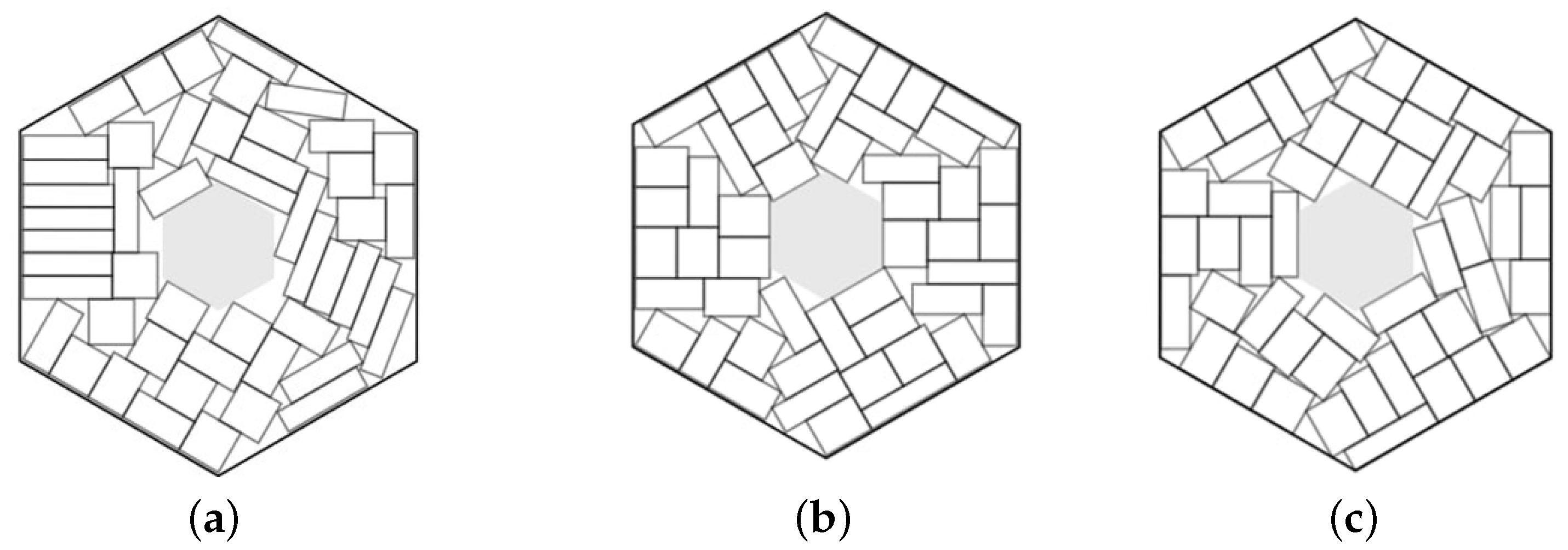
• Polygonal convex container given by its vertices $\lambda v_k^{\Omega }=(\lambda x_k^{\Omega },\lambda y_k^{\Omega }), k=1,\dots ,m$ with variable scaling parameter $\lambda \ge 0$, $L=\left\{\lambda \right\}$ (Figure 1):

  $$\Omega \left(\lambda \right)=\{(x,y)\in {\mathbb{R}}^2\left|min\{{\omega }_k^{\lambda }(x,y,\lambda ), k=1,\dots ,m\}\ge 0\right.\},$$

  where

  $${\omega }_k^{\lambda }(x,y,\lambda )=(y_k^{\Omega }-y_{k+1}^{\Omega })x+(-x_k^{\Omega }+x_{k+1}^{\Omega })y+\lambda (y_{k+1}^{\Omega }{x}_k^{\Omega }-x_{k+1}^{\Omega }{y}_k^{\Omega }),$$

  $$\lambda v_k^{\Omega }=(\lambda x_k^{\Omega },\lambda y_k^{\Omega }),k=1,\dots ,m,v_{m+1}^{\Omega }=v_1^{\Omega }.$$

Figure 1. Regular polygonal container $\Omega \left(\lambda \right)$ with scaling parameter $\lambda =1$, $\lambda =0.75$, and $\lambda =0.55$ (from the left to the right).

Figure 1. Regular polygonal container $\Omega \left(\lambda \right)$ with scaling parameter $\lambda =1$, $\lambda =0.75$, and $\lambda =0.55$ (from the left to the right).

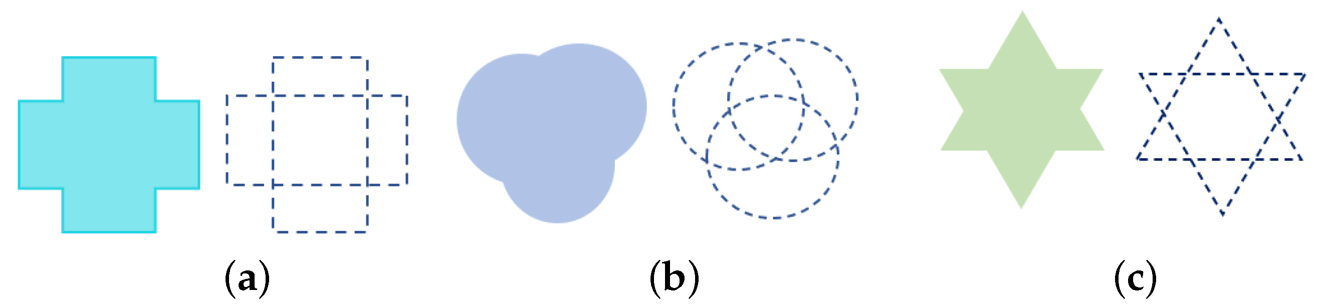
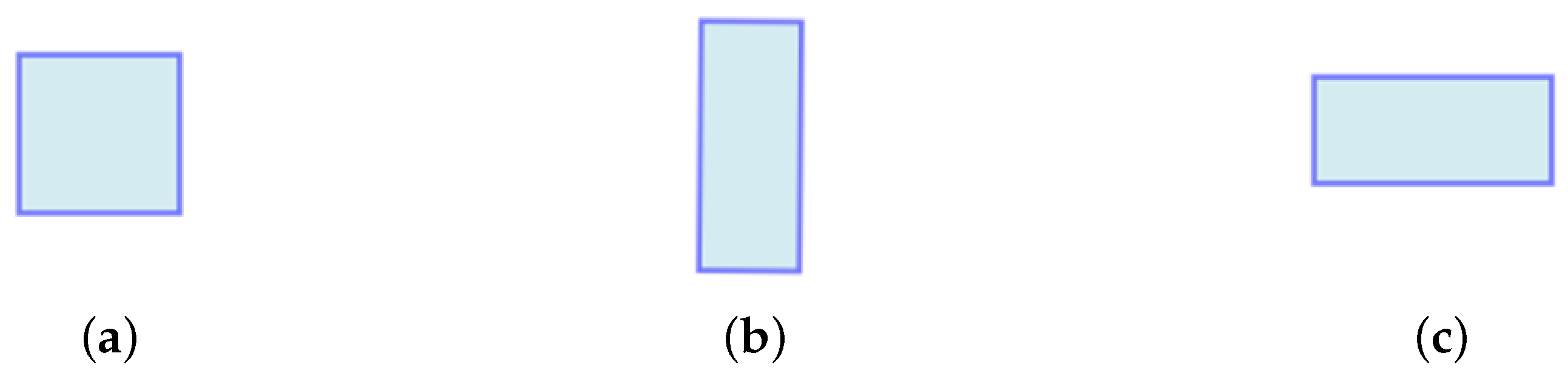
Prohibited zones. There may be some fixed configurations designed inside the container where the placement of the objects is prohibited. We refer to these configurations as prohibited zones. Denote a set of prohibited zones by {$P_z$, $z\in I_N=\{1,\dots ,N\}$}.

Each prohibited zone can be presented as a union of basic objects (circle, ellipse, rectangle, convex polygon) (Figure 2), i.e., $P_z\left(v_z\right)={\bigcup }_{j=1}^{n_z}{P}_{zj}\left(v_z\right)$ subject to the shape sizes and the position $v_z=(x_z,y_z)$ of the $P_z$ inside the container remain unchanged.

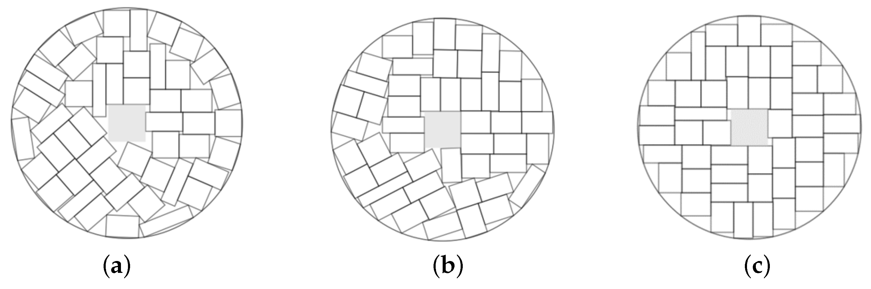
Figure 2. Examples of prohibited zones: (a) $P_1$ is a union of two rectangles; (b) $P_2$ is a union of three circles; (c) $P_3$ is a union of two triangles.

Figure 2. Examples of prohibited zones: (a) $P_1$ is a union of two rectangles; (b) $P_2$ is a union of three circles; (c) $P_3$ is a union of two triangles.

Soft rectangles. Let a set of rectangles $R_i=\{(x,y)\in {\mathbb{R}}^2{\left|-a_i\le x\le a_i, -b_i\le y\le b\right.}_i\},$$i\in I_n=\{1,\dots ,n\}$ be given in $XOY$.

Each rectangle $R_i$ can be rotated by an angle ${\theta }_i\in [0,2\pi )$, stretched by elasticity parameters ${\mu }_i^x,{\mu }_i^y\in R^{+}$ and translated by a vector $(x_i,y_i)\in {\mathbb{R}}^2$:

$$R_i(u_i,{\mu }_i)=\{p\in {\mathbb{R}}^2:p=(x_i,y_i)+A\left({\theta }_i\right)·M({\mu }_i^x,{\mu }_i^y)·p^0,\forall p^0\in R_i^0\},$$

(1)

where $R_i^0$ is the original rectangle with $x_i^0=0,$ $y_i^0=0,$ ${\theta }_i^0=0,$ ${\mu }_i^x={\mu }_i^y=1$, $A\left({\theta }_i\right)=\left(\begin{array}{cc}cos{\theta }_i& sin{\theta }_i\\ -sin{\theta }_i& cos{\theta }_i\end{array}\right)$ is a rotation matrix, $M\left({\mu }_i\right)=\left(\begin{array}{cc}{\mu }_i^x& 0\\ 0& {\mu }_i^y\end{array}\right)$ is an elasticity matrix, ${\mu }_i=({\mu }_i^x,{\mu }_i^y)$, $u_i=(x_i,y_i,{\theta }_i)$, $i\in I_n$.

The rectangle $R_i(u_i,{\mu }_i)$ defined by (1) is referred to as a soft rectangle.

Proposition 1.

The elasticity transformation preserves the area of the original rectangle $R_i$ under any translation and rotation iff ${\mu }_i^x{\mu }_i^y=1$. (See the proof in Appendix A).

Further, we assume that ${\mu }_i={\mu }_i^x$, ${\mu }_i^y=1/{\mu }_i$, ${\mu }^{-}\le {\mu }_i\le {\mu }^{+}$, ${\mu }^{-}\le {\mu }^{+}\in R^{+}$.

Figure 3 shows shapes of a soft rectangle for different values of elasticity coefficient ${\mu }_i$ subject to area preservation $S_i=S_i^0=8$.

Placement conditions. The following types of placement conditions are considered in this study:

(1)

Non-overlapping of each pair of soft rectangles:

$$int{R}_i(u_i,{\mu }_i)\cap int{R}_j(u_j,{\mu }_j)=Ø, (i,j)\in {\Lambda }^{\prime }=\{(i,j)\in I_n\times I_n,i>j\};$$

(2)

Containment of each soft rectangle into a convex container $\Omega \left(L\right)$:

$$R_i(u_i,{\mu }_i)\subset \Omega \left(L\right)\iff int{R}_i(u_i,{\mu }_i)\cap {\Omega }^{*}\left(L\right)=Ø,$$

$${\Omega }^{*}\left(L\right)={\mathbb{R}}^2\setminus int\Omega \left(L\right),i\in I_n;$$

(3)

Containment of each prohibited zone $T_z\left(v_z\right)$ into a convex container $\Omega \left(L\right)$:

$$P_z\left(v_z\right)\subset \Omega \left(L\right)\iff int{P}_z\left(v_z\right)\cap {\Omega }^{*}\left(L\right)=Ø;$$

(4)

Con-overlapping of each soft rectangle with prohibited zones:

$$int{P}_z\left(v_z\right)\cap int{R}_i(u_i,{\mu }_i)=Ø,z\in I_N=\{1,\dots ,N\},i\in I_n;$$

(5)

Metric constraints – ${\mu }^{-}\le {\mu }_i\le {\mu }^{+}$, ${\mu }^{-}\le {\mu }^{+}\in R^{+}$$i\in I_n$ represent given limits of the elasticity parameter.

Objective functions. Different objective functions are considered depending on the shape of the container $\Omega \left(L\right)$. That is, the height of a rectangular container, the radius of a circular container, and the scaling parameter of a polygonal container. Denote an objective function by $\kappa \left(L\right)$.

Problem formulation. The Optimized Packing Soft Rectangles (OPSR). Find an arrangement of soft rectangles $R_i(u_i,{\mu }_i)$, $i\in I_n$ minimizing $\kappa \left(L\right)$ subject to the placement conditions (1)–(5).

3. Mathematical Modeling

To describe the placement conditions of the OPSR problem, the phi-function technique [20,21] is used. For the reader’s convenience, basic definitions and properties of the phi-functions are provided in Appendix B.

3.1. Analytical Description of the Placement Conditions

Non-overlapping conditions. To define a non-overlapping condition (1) for soft rectangles $R_i(u_i,{\mu }_i)$ and $R_j(u_j,{\mu }_j)$, we introduce a quasi phi-function:

$${\Phi }_{ij}^{\prime }(u_i,u_j,{\mu }_i,{\mu }_j,{\tau }_{ij})=min\{{\Phi }^{R_i{H}_{ij}}(u_i,{\mu }_i,{\tau }_{ij}),{\Phi }^{R_j{H}_{ij}^{*}}(u_j,{\mu }_j,{\tau }_{ij})\}.$$

(2)

Here,

$${\Phi }^{R_i{H}_{ij}}(u_i,{\mu }_i,{\tau }_{ij})=\underset{1\le t\le 4}{min}(cos{\phi }_{ij}·x_{it}^{\prime }+sin{\phi }_{ij}·y_{it}^{\prime }+{\gamma }_{ij})$$

is a phi-function for objects $R_i(u_i,{\mu }_i)$ and $H\left({\tau }_{ij}\right)$,

$${\Phi }^{R_j{L}_{ij}^{*}}(u_j,{\mu }_j,{\tau }_{ij})=\underset{1\le l\le 4}{min}(-cos{\phi }_{ij}·x_{jl}^{\prime }-sin{\phi }_{ij}·y_{jl}^{\prime }-{\gamma }_{ij})$$

is a phi-function for objects $R_j(u_j,{\mu }_j)$ and $H_{ij}^{*}\left({\tau }_{ij}\right)={\mathbb{R}}^2\setminus L_{ij}\left({\tau }_{ij}\right)$, where

$$H_{ij}\left({\tau }_{ij}\right)=\left\{(x,y): {\psi }_{ij}=cos{\phi }_{ij}·x+sin{\phi }_{ij}·y+{\gamma }_{ij}\le 0\right\},$$

${\tau }_{ij}=({\phi }_{ij},{\gamma }_{ij})\in {\mathbb{R}}^2$ is a vector of variable parameters of $H_{ij}\left({\tau }_{ij}\right)$, and

$$x_{it}^{\prime }=({\mu }_i^x{\tilde{x}}_{it}·cos{\theta }_i-{\mu }_i^y{\tilde{y}}_{it}·sin{\theta }_i),y_{it}^{\prime }=({\mu }_i^x{\tilde{x}}_{it}·sin{\theta }_i+{\mu }_i^y·{\tilde{y}}_{it}·cos{\theta }_i),t=1,\dots ,4$$

are coordinates of vertices of soft rectangle $R_i(x_i,y_i,{\theta }_i,{\mu }_i)$.

Thus, if ${\Phi }_{ij}^{\prime }(u_i,u_j,{\tau }_{ij},{\mu }_i,{\mu }_j)\ge 0$ for some ${\tau }_{ij}^{\prime }=({\phi }_{ij},{\gamma }_{ij})$, then soft rectangles do not overlap, i.e., $int{R}_i(x_i,y_i,{\theta }_i,{\mu }_i)\cap int{R}_j(x_j,y_j,{\theta }_j,{\mu }_j)=Ø$.

We state non-overlapping condition (3) for a soft rectangle $R_i(u_i,{\mu }_i)$ and a fixed prohibited zone $P_z\left(v_z\right)={\displaystyle \bigcup _{j=1}^{n_z}}{P}_{zj}\left(v_z\right)$ using the following quasi phi-function:

$${\Phi }_{iz}^{\prime }(u_i,u_z,{\mu }_i,{\tau }_{iz})=min\{{\Phi }^{\prime R_i{P}_{zj}}(u_i,u_z,{\mu }_i,{\tau }_{ij}^z),j\in J_z\},$$

(3)

where ${\Phi }^{\prime R_i{P}_{zj}}(u_i,u_z,{\mu }_i,{\tau }_{ij}^z)$ is a quasi phi-function for objects $P_{zj}\left(v_z\right)$ and $R_i(u_i,{\mu }_i)$, ${\tau }_{iz}=({\tau }_{ij}^z,j\in J_z=\{1,\dots ,n_z\})$.

Thus, if ${\Phi }_{iz}^{\prime }(u_i,u_z,{\mu }_i,{\tau }_{iz})\ge 0$ for some ${\tau }_{iz},j\in J_z$, then $P_{zj}\left(v_z\right)$ and $R_i(u_i,{\mu }_i)$ do not overlap, i.e., $int{R}_i(u_i,{\mu }_i)\cap int{P}_z\left(v_z\right)=Ø$.

Containment conditions. Let us consider the containment condition (2) that describes the relation $R_i(u_i,{\mu }_i)\subset$$\Omega \left(L\right)$, i.e., ${intR}_i(u_i,{\mu }_i)\cap {\Omega }^{*}\left(L\right)=Ø$, ${\Omega }^{*}\left(L\right)={\mathbb{R}}^2\setminus int\Omega \left(L\right)$, using a phi-function, denoted by ${\Phi }_i(u_i,{\mu }_i,L)$, for objects $R_i(u_i,{\mu }_i)$ and ${\Omega }^{*}\left(L\right)$.

If $\Omega (L=(l,h\left)\right)$ is a rectangular container, then

$${\Phi }_i^{\prime }(u_i,{\mu }_i,l,h)=\underset{t=1,\dots ,4}{min}{\omega }_{it}(u_i,{\mu }_i,l,h),$$

(4)

where

$${\omega }_{i1}(u_i,{\mu }_i,l,h)=({\mu }_i^x{x}_{it}·cos{\theta }_i-{\mu }_i^y{y}_{it}·sin{\theta }_i)+x_i,$$

$${\omega }_{i2}(u_i,{\mu }_i,l,h)=-({\mu }_i^x{x}_{it}·cos{\theta }_i-{\mu }_i^y(y_{it}·sin{\theta }_i))-x_i+l,$$

$${\omega }_{i3}(u_i,{\mu }_i,l,h)=({\mu }_i^x{x}_{it}·sin{\theta }_i+{\mu }_i^y(y_{it}·cos{\theta }_i))+y_i,$$

$${\omega }_{i4}(u_i,{\mu }_i,l,h)=-({\mu }_i^x{x}_{it}·sin{\theta }_i+{\mu }_i^y(y_{it}·cos{\theta }_i))-y_i+h$$

If $\Omega (L=r)$ is a circular container, then

$${\Phi }_i^{\prime }(u_i,{\mu }_i,r)=-(X_i^2+Y_i^2)+r^2,i\in I_n,$$

(5)

where

$$X_i=({\mu }_i^x{x}_{it}·cos{\theta }_i-{\mu }_i^y{y}_{it}·sin{\theta }_i)+x_i,Y_i=({\mu }_i^x{x}_{it}·sin{\theta }_i+{\mu }_i^y{y}_{it}·cos{\theta }_i)+y_i,t=1,\dots ,4.$$

If $\Omega (L=\lambda )$ is a scaling convex polygonal container, then

$${\Phi }_i^{\prime }(u_i,{\mu }_i,\lambda )=\underset{k=1,\dots ,m}{min}({\alpha }_k{\tilde{y}}_{it}+{\beta }_k{\tilde{x}}_{it}+\lambda {\gamma }_k),$$

(6)

$${\alpha }_k=(-x_k^{\Omega }+x_{k+1}^{\Omega }), {\beta }_k=(y_k^{\Omega }-y_{k+1}^{\Omega }), {\gamma }_k=(y_{k+1}^{\Omega }{x}_k^{\Omega }-x_{k+1}^{\Omega }{y}_k^{\Omega }),$$

where $v_k^{\Omega }=(x_k^{\Omega }, y_k^{\Omega }), k=1,\dots ,m$, $X_{m+1}^{\Omega }=X_1^{\Omega }$,

$${\tilde{x}}_{it}=({\mu }_i^x{x}_{it}·cos{\theta }_i-{\mu }_i^y{y}_{it}·sin{\theta }_i)+x_i,{\tilde{y}}_{it}=({\mu }_i^x{x}_{it}·sin{\theta }_i+{\mu }_i^y{y}_{it}·cos{\theta }_i)+y_i,t=1,\dots ,4.$$

Thus, the inequality ${\Phi }_i(u_i,{\mu }_i,L)\ge 0$ provides containment of a soft rectangle $R_i(u_i,{\mu }_i)$ into a container $\Omega \left(L\right)$, i.e., $R_i(u_i,{\mu }_i)\subset \Omega \left(L\right)$ for $i\in I_n$.

Containment condition (3) for prohibited zones $P_z\left(v_z\right)={\displaystyle \bigcup _{j=1}^{n_z}}{P}_{zj}\left(v_z\right)$, i.e., $P_z\left(v_z\right)$$\subset \Omega \left(L\right)$, $z\in {\mathrm{I}}_N$ can be described using phi-functions/quasi phi-functions for objects $P_z\left(v_z\right)$ and ${\Omega }^{*}\left(L\right)$ in the form

$${\Phi }_z^{″}(v_z,L)=min\{{\Phi }_{zj}^{″}(v_z,L),j\in J_z=\{1,\dots ,n_z\}\}$$

(7)

where ${\Phi }_{zj}^{\prime \prime }(v_z,L)$ is a phi-function/quasi phi-function for a convex component $P_{zj}\left(v_z\right)\subset P_z\left(v_z\right)$ and the object ${\Omega }^{*}\left(L\right)$.

Ready-to-use phi-functions/quasi phi-functions for the complement of the container (rectangular, circular, or polygonal) and a convex component $P_{zj}\left(v_z\right)$ can be found, e.g., in [20,22].

Thus, the inequality ${\Phi }_z^{\prime \prime }(v_z,L)\ge 0$ ensues the containment of a prohibited zone $P_z\left(v_z\right)$ into a container $\Omega \left(L\right)$, i.e., $P_z\left(v_z\right)\subset \Omega \left(L\right)$ for $z\in {\mathrm{I}}_N$.

3.2. Mathematical Model

The OPSR problem can be stated as the following nonlinear programming model:

$$\underset{(u,\tau ,\mu ,L)}{min}\kappa \left(L\right)$$

(8)

subject to

$${\Phi }_{ij}^{\prime }(u_i,u_j,{\mu }_i,{\mu }_j,{\tau }_{ij})\ge 0,(i,j)\in {\Lambda }^{\prime },$$

(9)

$${\Phi }_{iz}^{\prime \prime }(u_i,u_z,{\mu }_i,{\tau }_{ij}^z)\ge 0,(i,j)\in {\Lambda }^{\prime \prime },$$

(10)

$${\Phi }_i^{\prime }(u_i,{\mu }_i,L)\ge 0,i\in I_n,$$

(11)

$${\Phi }_z^{\prime \prime }(u_z,L)\ge 0,z\in I_N,$$

(12)

$${\mu }^{-}<{\mu }_i\le {\mu }^{+},i\in I_n,$$

(13)

where $\kappa \left(L\right)$ is an objective function that depends on variable dimensions L of a container;

$u=(u_i,i\in I_n)$, ${\tau }_{ij}=({\varphi }_{ij},{\gamma }_{ij})$ for $(i,j)\in {\Lambda }^{\prime }$, ${\Lambda }^{\prime }=\{(i,j):i>j\in I_n\},$ $\tau =({\tau }_{ij},(i,j)\in {\Lambda }^{\prime },$ ${\tau }_{ij}^z$, $(i,j)\in {\Lambda }^{\prime \prime }$), ${\tau }_{ij}^z=({\varphi }_{ij}^z,{\gamma }_{ij}^z),$ ${\Lambda }^{\prime \prime }=\{(i,j):i\in I_n,j\in J_z,z\in I_N\},$$\mu =({\mu }_i,i\in I_n)$.

Inequalities (9) and (10) describe the non-overlapping of a pair of soft rectangles/a soft rectangle and a prohibited zone; inequalities (11) and (12) state the containment of a soft rectangle/a prohibited zone into a container; inequality (13) restricts a level of elasticity of soft rectangles.

${\Phi }_{ij}^{\prime }(u_i,u_j,{\mu }_i,{\mu }_j,{\tau }_{ij})$ is defined by (2), ${\Phi }_{iz}^{\prime \prime }(u_i,u_z,{\mu }_i,{\tau }_{ij}^z)$ is defined by (3), ${\Phi }_i^{\prime }(u_i,{\mu }_i,L)$ is defined by (4)–(6), ${\Phi }_z^{\prime \prime }(v_z,L)$ is defined by (7), and $d=4n+n(n-1)+2n{\displaystyle \sum _{z=1}^N}{n}_z+\left|L\right|$ is the total number of the problem variables.

4. A Heuristic Approach to Solve OPSR Problems

To apply state-of-the-art NLP local solvers for the large-scale nonconvex optimization problem (8)–(13) (subject to a balance between computational time and solution quality), we need to cope with two challenging issues: (1) how to construct feasible starting points (critical for most local NLP solvers); (2) how to reduce the problem dimension.

To find feasible starting points of the problem (8)–(13), we develop an algorithm based on homothetic transformations of spheres. To answer the second question, we propose a decomposition technique based on the results of [23] that allows reducing the large-scale problem (8)–(13) to a sequence of nonlinear programming subproblems of much smaller dimensions (increasing linearly to the number of soft rectangles $R_i(u_i,{\mu }_i)$), subject to ${\mu }^{-}<{\mu }_i\le {\mu }^{+}$, $i\in I_n$.

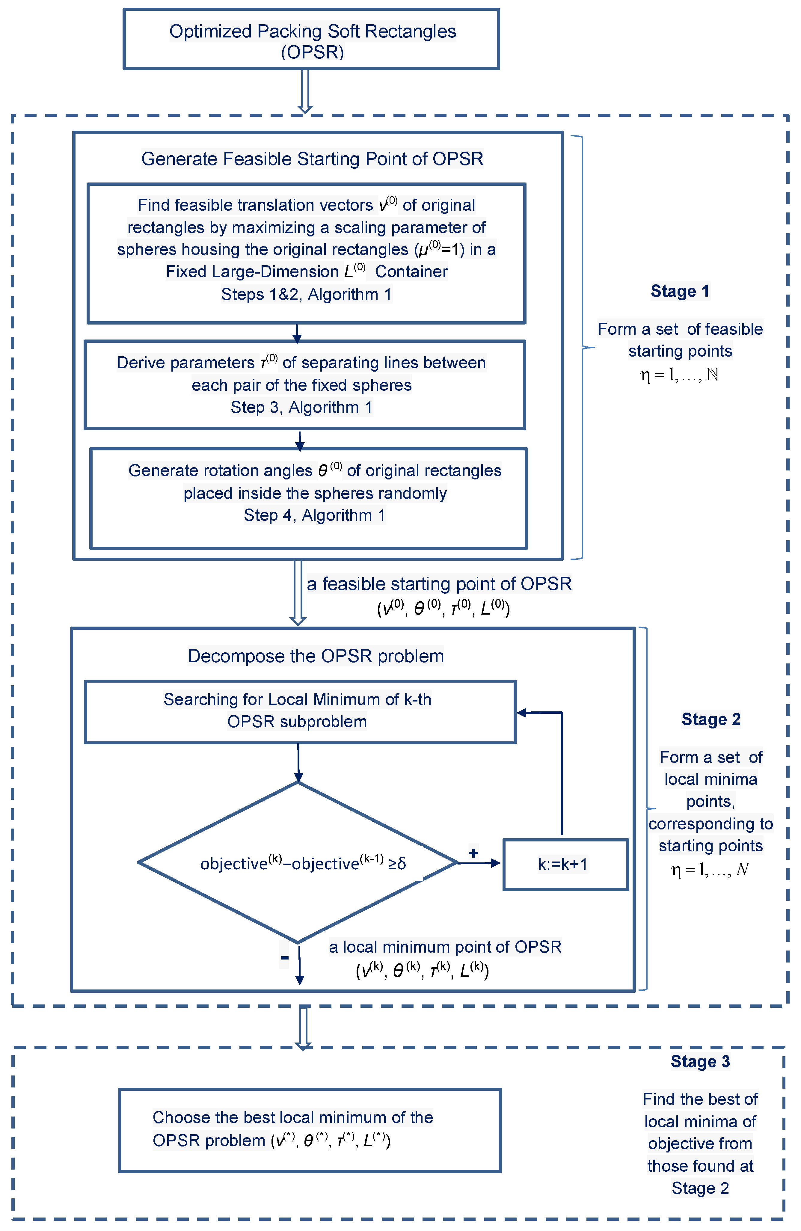
Our multistart heuristic approach consists of three main stages:

Stage 1. Generating feasible starting points of the problem (8)–(13) using Algorithm 1.

Stage 2. Searching for a local minimum of the problem (8)–(13) using Algorithm 2.

Stage 3. Selecting the best result from those found at Stage 2.

Let us consider the algorithm of generating feasible starting points of the problem (8)–(13) used at the first stage of the strategy.

Algorithm 1. Firstly, we circumscribe a sphere $S_i$ around each fixed original rectangle $R_i$ for $i\in I_n$. Assume that the center $v_i$ of the sphere $S_i$ is arranged at the center of rectangle $R_i$ (the midpoint of its diagonal end points). Secondly, we set starting dimensions $L^0$ of a container $\Omega \left(L\right)$ sufficiently large to host prohibited zones $P_z$, $z\in I_N$, as well as all spheres $S_i\left(v_i\right)$, $i\in I_n$.

Step 1. Generate randomly n centers $v_i^0=(x_i^0,y_i^0)$ of spheres $S_i$ subject to $v_i^0\in {\Omega }^z\left(L^0\right)=\Omega \left(L^0\right)/{\displaystyle \bigcup _z^N}{P}_z$ for $i\in I_n$ that can be considered as a set of n degenerated spheres placed inside the container ${\Omega }^z\left(L^0\right)$.

Solve the problem of maximizing the homothety coefficient (scaling parameter) $\rho$ of the non-overlapping spheres $S_i(v_i,\rho )$, $i\in I_n,$ so that they do not overlap with prohibited zones $P_z$, $z\in I_N$ and fit the container ${\Omega }^z\left(L^0\right)$, using the starting feasible point $(v^0,{\rho }^0)$, $v^0=(v_i^0,i\in I_n)$, ${\rho }^0=0.$.

This optimization problem can be stated as the following nonlinear programming model:

$$\underset{v,\rho }{max}\rho$$

subject to

$${\psi }_i^{\prime }(v_i,\rho ,L)\ge 0,i\in I_n,$$

$${\phi }_{ij}^{\prime }(v_i,v_j,\rho )\ge 0,(i,j)\in {\Lambda }^{\prime },$$

$${\phi }_{iz}^{\prime \prime }(v_i,v_z,\rho )\ge 0,i\in I_n,z\in I_N,$$

$$0\le \rho \le 1,v_i=(x_i,y_i),i\in I_n,$$

where $(v,\rho )=\left(v_1,\dots ,v_n,\rho \right)$ is a vector of the decision variables, the inequality ${\psi }_i^{\prime }(v_i,\rho ,L)\ge 0$ describes the containment of a scaling sphere $\rho S_i\left(v_i\right)$ into a container $\Omega \left(L\right)$, i.e., $\rho S_i\left(v_i\right)\subset \Omega \left(L\right)$, the inequality ${\phi }_{ij}^{\prime }(v_i,v_j,\rho )\ge 0$ ensures the non-overlapping of two scaling spheres $\rho S_i\left(v_i\right)$ and $\rho S_j\left(v_j\right)$, i.e., $int\rho S_i\left(v_i\right)\cap int\rho S_j\left(v_j\right)=Ø$, while the inequality ${\phi }_{iz}^{\prime \prime }(v_i,v_z,\rho )\ge 0$ holds the non-overlapping of a scaling sphere $\rho S_i\left(v_i\right)$ and a prohibited zone $P_z\left(v_z\right)$, i.e., $int\rho S_i\left(v_i\right)\cap int{P}_z\left(v_z\right)=Ø$. In the model, functions ${\psi }_i^{\prime }$, ${\phi }_{ij}^{\prime }$, and ${\phi }_{iz}^{\prime \prime }$ are ready-to-use phi-functions for the appropriate pair of objects that can be found, e.g., in [20,22].

Denote a point of local maximum of the problem by $(v^{\prime },{\rho }^{\prime })$, $v^{\prime }=(v_1^{\prime },\dots ,v_n^{\prime })$.

The solution ${\rho }^{\prime }=1$ corresponds to the original sizes of the spheres.

Step 2. If ${\rho }^{\prime }=1$, then Step 3; if ${\rho }^{\prime }<1$, then take a larger value for $L^0$ and go to Step 1.

Step 3. Derive feasible values of auxiliary variables ${\tau }_{ij}^{\prime }=({\varphi }_{ij}^{\prime },{\gamma }_{ij}^{\prime })\in {\mathbb{R}}^2$, $(i,j)\in {\Lambda }^{\prime }$ and ${\tau }_{ij}^{\prime z}=({\varphi }_{ij}^{\prime z},{\gamma }_{ij}^{\prime z})\in {\mathbb{R}}^2$, $(i,j)\in {\Lambda }^{\prime \prime }$ subject to fixed centers of spheres $S_i(v_i^{\prime },{\rho }^{\prime })$, $i\in I_n$, and $S_{zj}\left(v_z\right)$, $j\in J_z$, $z\in I_N$ using simple geometric constructions of separating lines between each pair of spheres.

Step 4. Randomly generate rotation angles ${\theta }_i^{\prime }\in \left[0,2\pi \right)$, $i\in I_n$ for the corresponding rectangles. Substitute spheres $S_i(v_i^{\prime },{\rho }^{\prime }=1)$ by the corresponding rectangles $R_i(v_i^{\prime },{\theta }_i^{\prime },{\mu }_i^{\prime })$ for ${\mu }_i^{\prime }=1$, $i\in I_n$.

The algorithm returns point $(u^{\prime },{\tau }^{\prime },{\mu }^{\prime },L^{\left(0\right)})$ as a feasible starting point of the problem (9)–(14) for further local optimization, where $u^{\prime }=(u_i^{\prime },i\in I_n)$, $u_i^{\prime }=(v_i^{\prime },{\theta }_i^{\prime })$, ${\tau }_{ij}^{\prime }=({\varphi }_{ij}^{\prime },{\gamma }_{ij}^{\prime })$, ${\tau }^{\prime }=({\tau }_{ij}^{\prime },(i,j)\in {\Lambda }^{\prime },{\tau }_{ij}^{\prime z}$, $(i,j)\in {\Lambda }^{\prime \prime })$, ${\tau }_{ij}^{\prime z}=({\varphi }_{ij}^{\prime z},{\gamma }_{ij}^{\prime z}),$${\mu }^{\prime }=({\mu }_i^{\prime }=1,i\in I_n)$.

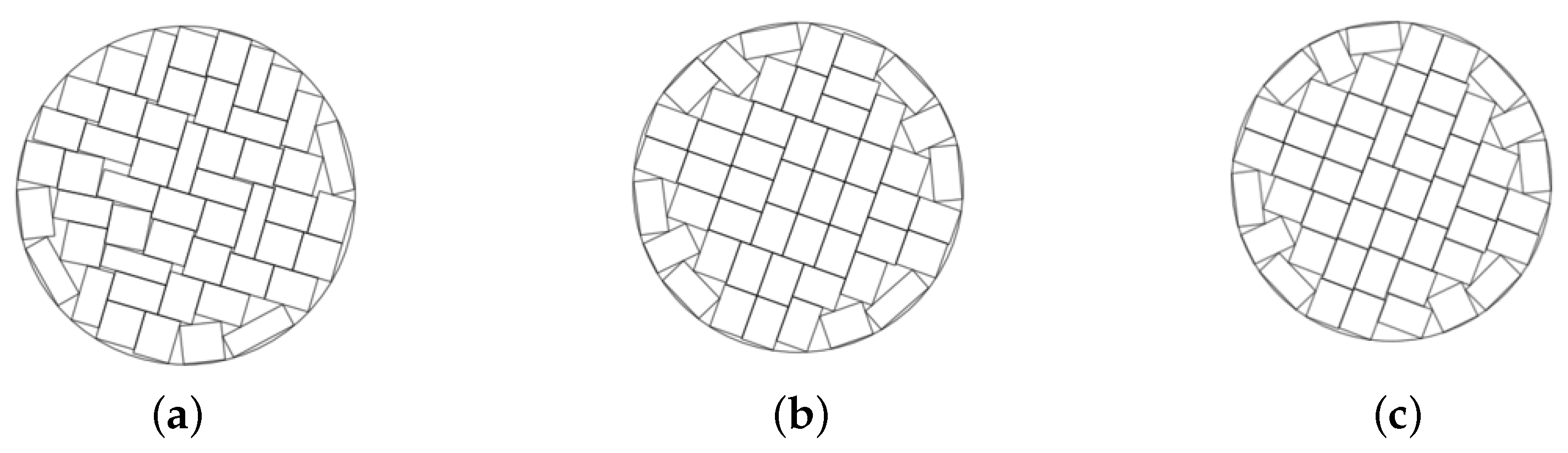
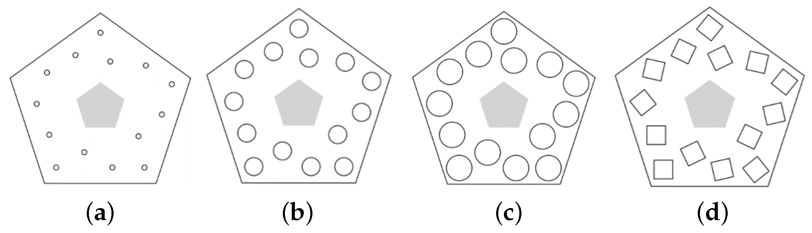
Figure 4a–c show some iterations of growing spheres $\rho S_i\left(v_i\right)$ in the optimization procedure at Step 1 for a polygonal container $\Omega \left({\lambda }^0\right)$ with increasing values of $\rho$. The configuration shown in Figure 4d corresponds to a global solution of the problem considered at Step 1.

To search for local-optimal solutions of the OPSP problem (8)–(13), we propose a decomposition strategy that involves the following steps.

Algorithm 2. Let $(u^{\left(0\right)},{\tau }^{\left(0\right)},{\mu }^{\left(0\right)},L^{\left(0\right)})$ be a feasible starting point found by Algorithm 1, where $u^{\left(0\right)}=u^{\prime }, {\tau }^{\left(0\right)}={\tau }^{\prime }, {\mu }^{\left(0\right)}=({\mu }_i^{\prime }=1, i\in I_n$).

Step 1. Set $k=0$.

Step 2. Set ${\epsilon }_{\mu }={\mu }^{+}·\underset{i\in I_n}{max}{r}_i$ and form ${\epsilon }_{\mu }$-neighborhood

$${\Omega }_i^{\left(k\right)}\left(\mu \right)=\{(x,y):x_i^{\left(k\right)}-(r_i+{\epsilon }_{\mu })\le x\le x_i^{\left(k\right)}+(r_i+{\epsilon }_{\mu }),$$

$$y_i^{\left(k\right)}-(r_i+{\epsilon }_{\mu })\le y\le y_i^{\left(k\right)}+(r_i+{\epsilon }_{\mu })\}.$$

Step 3. Define placement conditions on the vector $v_i$ of $S_i\left(v_i\right)$, $i\in I_n$

$$f_i^{\left(k\right)}\left(v_i\right)=min\{-x_i+x_i^{\left(k\right)},x_i-x_i^{\left(k\right)},-y_i+y_i^{\left(k\right)},y_i-y_i^{\left(k\right)}\}+{\epsilon }_{\mu }\ge 0.$$

(14)

Step 4. Form a feasible region $W^{(k+1)}$ for $(k+1)$-th subproblem:

$$W^{(k+1)}=\{(u,\tau ,\mu ,L)\in {\mathbb{R}}^{d-d^{\left(k\right)}}:{\Phi }^{\prime }(u_i,u_j,{\mu }_i,{\mu }_j,{\tau }_{ij})\ge 0,\left(i,j\right)\in {\Lambda }^{\prime \left(k\right)},$$

$${\Phi }_{iz}^{\prime \prime }(u_i,u_z,{\mu }_i,{\tau }_{ij}^z)\ge 0,{\Phi }_i^{\prime }\left(u_i,{\mu }_i,L\right)\ge 0,i\in I_n,{\Phi }_z^{\prime \prime }(u_z,L)\ge 0,z\in I_N,f_i^{\left(k\right)}\left(v_i\right)\ge 0,i\in I_n\},$$

where ${\Lambda }^{\prime \left(k\right)}=\{(i,j)\in {\Lambda }^{\prime }:∥v_i^{\left(k\right)}-v_j^{\left(k\right)}∥\le d_{ij}\}$, ${\Lambda }^{\prime \prime \left(k\right)}=\{(i,j)\in {\Lambda }^{\prime \prime }:∥v_i^{\left(k\right)}-v_{zj}^{\left(k\right)}∥\le d_{ij}^z\}, d_{ij}=\sqrt{2}(r_i+r_j+2{\epsilon }_{\mu })$, $d_{ij}^z=\sqrt{2}(r_i+r_{zj}+2{\epsilon }_{\mu })$, $d^{\left(k\right)}=m-2m^{\left(k\right)}$, $m=m_1+m_2, m_1=\left|{\Lambda }^{\prime }\right|=n(n-1)/2, m_2=\left|{\Lambda }^{\prime \prime }\right|=n{\displaystyle \sum _{z=1}^N}{n}_z$, $m^{\left(k\right)}=\left|{\Lambda }^{\prime \left(k\right)}\right|+\left|{\Lambda }^{\prime \prime \left(k\right)}\right|$.

Then, we eliminate from (9) and (10) the phi-function inequalities for each pair $(i,j)\in {\Lambda }^{\prime }$ of objects if $∥v_i^{\left(k\right)}-v_j^{\left(k\right)}∥>d_{ij}$, while a system of linear inequalities $-x_i+x_i^{\left(k\right)}\ge 0,$$x_i-x_i^{\left(k\right)}\ge 0,$$-y_i+y_i^{\left(k\right)}\ge 0,$$y_i-y_i^{\left(k\right)}\ge 0$ defined by (14) is added to the system (10)–(14) for $i\in I_n$.

This technique allows reducing the number of variables by $d^{\left(k\right)}$ while the number of nonlinear inequalities in (9) and (10) is reduced by $m^{\left(k\right)}$.

Step 5. Search for a local-optimal solution of the $(k+1)$- subproblem

$$\underset{(u,{\tau }^{\left(k\right)},\mu ,L)}{min}\kappa \left(L\right)$$

(15)

subject to

$${\Phi }_{ij}^{\prime }(u_i,u_j,{\mu }_i,{\mu }_j,{\tau }_{ij})\ge 0,(i,j)\in {\Lambda }^{\prime \left(k\right)},$$

(16)

$${\Phi }_{iz}^{\prime \prime }(u_i,u_z,{\mu }_i,{\tau }_{ij}^z)\ge 0,(i,j)\in {\Lambda }^{\prime \prime \left(k\right)},$$

(17)

$${\Phi }_i^{\prime }(u_i,{\mu }_i,L)\ge 0,i\in I_n,$$

(18)

$${\Phi }_z^{\prime \prime }(u_z,L)\ge 0,z\in I_N,$$

(19)

$$f_i^{\left(k\right)}\left(v_i\right)\ge 0,i\in I_n,$$

(20)

$$\kappa \left(L\right)\le \kappa \left(L^{\left(k\right)}\right),$$

(21)

$${\mu }^{-}<{\mu }_i\le {\mu }^{+},$$

(22)

$$u=(u_i,i\in I_n),u_i=(x_i,y_i,{\theta }_i),{\tau }^{\left(k\right)}=({\tau }_{ij},(i,j)\in {\Lambda }^{\left(k\right)}),{\tau }_{ij}=({\varphi }_{ij},{\gamma }_{ij}).$$

Denote a point of local minimum of the problem (15)–(22) by $(u^{*(k+1)},{\mu }^{*(k+1)},L^{*(k+1)})$.

Step 6. If $\left|\kappa {\left(L\right)}^{*(k+1)}-\kappa {\left(L\right)}^{*\left(k\right)}\right|\ge \delta$, then go to Step 7; otherwise, stop the algorithm.

Step 7. Set $k=k+1$ and go to Step 2.

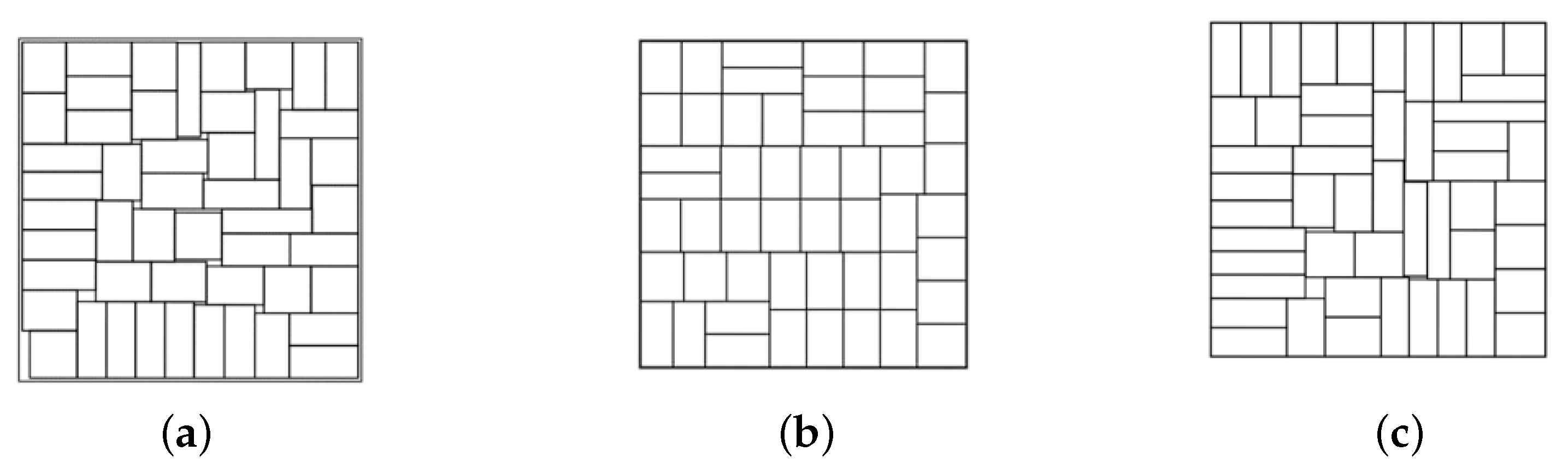
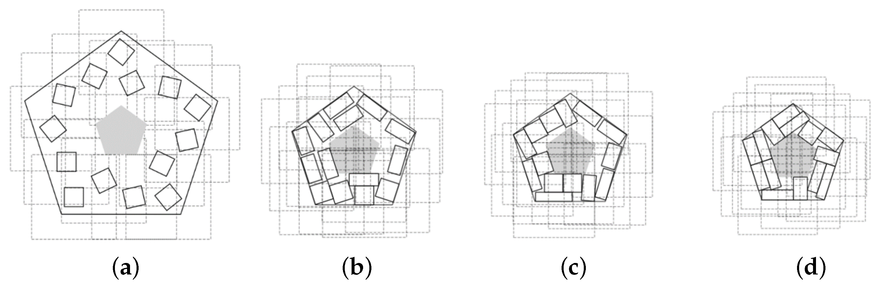
Figure 5 provides illustrations of the decomposition procedure in Algorithm 2 for optimized packing of soft rectangles in a scaling regular pentagon $\Omega \left(\lambda \right)$ with a polygonal prohibited area.

The configuration (a) corresponds to the feasible starting point found by Algorithm 1, $k=0$. The configurations (b)–(d) corresponds to local optimal solutions of three subproblems (15)–(22), $k=1,2,3$. The configuration (d) correspond to a local minimum of the problem (15)–(22) found at the last iteration $k=3$ (${\lambda }^{\left(2\right)}-{\lambda }^{\left(3\right)}<\delta =0.01$, Step 6) of the decomposition procedure.

Figure 6 presents a flow chart of the proposed heuristic approach for solving the OPSR problem.

5. Computational Results

In computational experiments, a computer was used having the processor 12th Gen Intel Core i5-12500 3.00 GHz. RAM 32 GB. Programming Language Python 3.11 was used for programming the algorithms. To solve nonlinear programming subproblems (15)–(22), a non-commercial local NLP solver, IPOPT (version 3.14.14) [24], was applied.

Two groups of instances for packing soft rectangles with different limits of the elasticity parameter ${\mu }_i^{-}\le {\mu }_i\le {\mu }_i^{+},i\in I_n$ in three types of containers (circular, rectangular, and polygonal) were considered: (1) without prohibited zones (Examples 1–7, Figure 2 and Figure 7, Figure 8, Figure 9, Figure 10, Figure 11, Figure 12 and Figure 13) with prohibited zones (Examples 8–15, Figure 14, Figure 15, Figure 16, Figure 17, Figure 18, Figure 19, Figure 20 and Figure 21). Specific values of the elasticity parameters for all problem instances considered in the paper can be found at ResearchGate https://www.researchgate.net/publication/388143731_elasticity_parameters (accessed on 1 January 2025). Three feasible starting points are used for each instance. The CPU time limit in both cases was 300 s.

The following notations are used in presenting experimental results:

n: the number of soft rectangles;

m: the number of the polygonal container vertices;

$L^{*}$: an optimized size of a container (the best value of the objective function $\kappa \left(L\right)$ found by our heuristic for ${\mu }_i^{-}\le {\mu }_i\le {\mu }_i^{+},i\in I_n$), i.e., $r^{*}$: for circular container $\Omega \left(r\right)$, $h^{*}$: for rectangular container $\Omega (l,h)$, ${\lambda }^{*}$: for polygonal container $\Omega \left(\lambda \right)$;

$f^{*}$ denotes $afilling factor={\displaystyle \frac{a total area of soft rectangles}{an optimized area of container \Omega \left(L^{*}\right)}}$ in %.

5.1. Instances Without Prohibited Zones

In this subsection different minimum scale regular containers are considered for packing soft rectangles.

Example 1.

$n=50$, total area of rectangles is 400, circular container.

Figure 7. The best solutions in Example 1: (a) $1\le {\mu }_i\le 2, r^{*}=11.9$, $f^{*}=89.96\%$; (b) $0.5\le {\mu }_i\le 1.5$, $r^{*}=11.88$, $f^{*}=90.26\%$; (c) $0.3\le {\mu }_i\le 2.5, r^{*}=11.86$, $f^{*}=90.56$%.

Figure 7. The best solutions in Example 1: (a) $1\le {\mu }_i\le 2, r^{*}=11.9$, $f^{*}=89.96\%$; (b) $0.5\le {\mu }_i\le 1.5$, $r^{*}=11.88$, $f^{*}=90.26\%$; (c) $0.3\le {\mu }_i\le 2.5, r^{*}=11.86$, $f^{*}=90.56$%.

Example 2.

$n=50$, $h=l$, total area of rectangles is 400, square container.

Figure 8. The best solutions in Example 2: (a) $1\le {\mu }_i\le 2, h^{*}=20.1385, f^{*}=98.63\%$; (b) $0.3\le {\mu }_i\le 1.5$, $h^{*}=20.003, f^{*}=99.97\%$; (c) $0.5\le {\mu }_i\le 2.5, h^{*}=20.0592, f^{*}=99.41\%$.

Figure 8. The best solutions in Example 2: (a) $1\le {\mu }_i\le 2, h^{*}=20.1385, f^{*}=98.63\%$; (b) $0.3\le {\mu }_i\le 1.5$, $h^{*}=20.003, f^{*}=99.97\%$; (c) $0.5\le {\mu }_i\le 2.5, h^{*}=20.0592, f^{*}=99.41\%$.

Example 3.

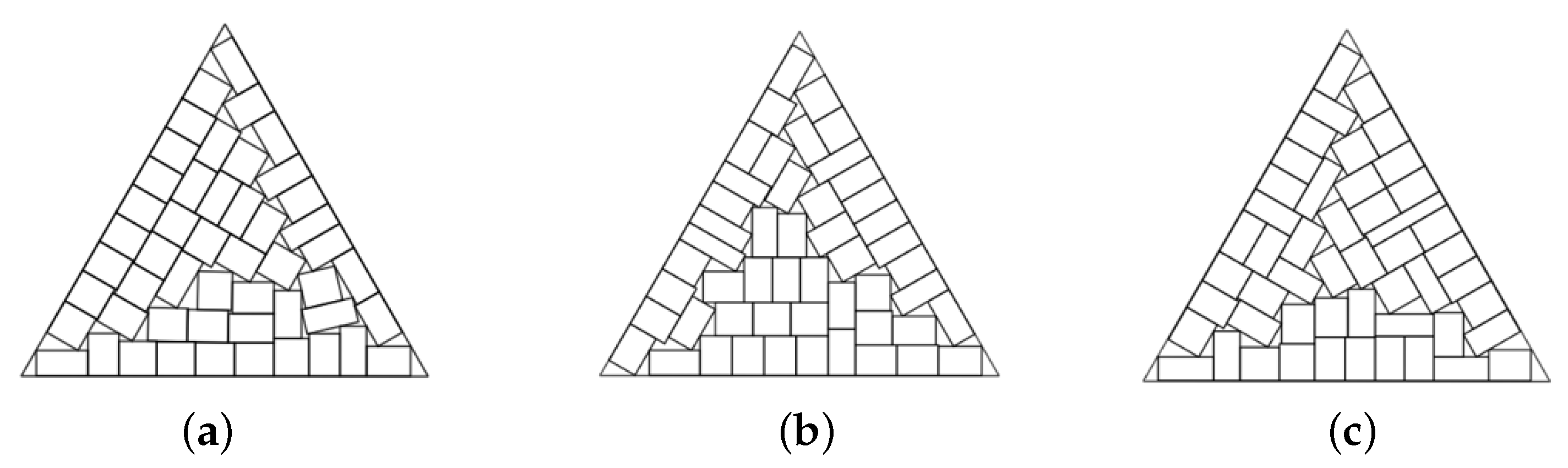
$n=50$, $m=3$, total area of rectangles is 400, triangular container.

Figure 9. The best solutions in Example 3: (a) $1\le {\mu }_i\le 2, {\lambda }^{*}=0.46, f^{*}=90.95\%$; (b) $0.5\le {\mu }_i\le 1.5$, ${\lambda }^{*}=0.457, f^{*}=92.15\%$; (c) $0.8\le {\mu }_i\le 2.5, {\lambda }^{*}=0.459, f^{*}=91.35\%$.

Figure 9. The best solutions in Example 3: (a) $1\le {\mu }_i\le 2, {\lambda }^{*}=0.46, f^{*}=90.95\%$; (b) $0.5\le {\mu }_i\le 1.5$, ${\lambda }^{*}=0.457, f^{*}=92.15\%$; (c) $0.8\le {\mu }_i\le 2.5, {\lambda }^{*}=0.459, f^{*}=91.35\%$.

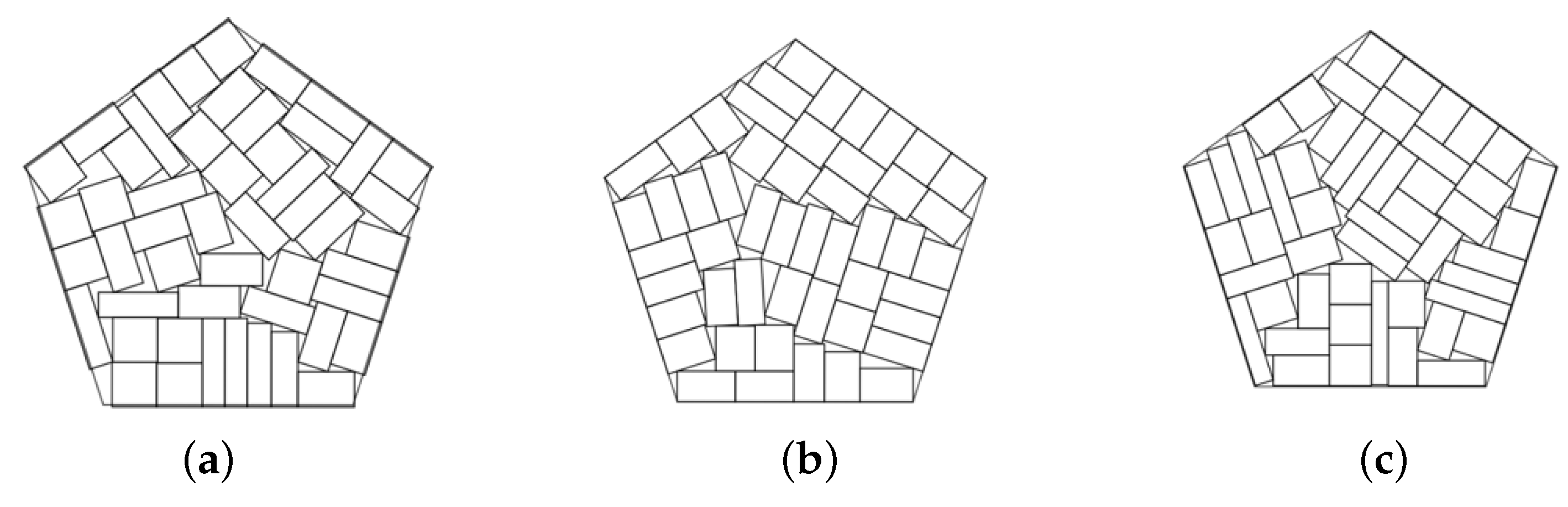
Example 4.

$n=50$, $m=5$, total area of rectangles is 400, pentagonal container.

Figure 10. The best solutions in Example 4: (a) $1\le {\mu }_i\le 2, {\lambda }^{*}=0.34, f^{*}=90.95\%$; (b) $0.5\le {\mu }_i\le 1.5$, ${\lambda }^{*}=0.336, f^{*}=93.14\%$; (c) $0.5\le {\mu }_i\le 2.5, {\lambda }^{*}=0.334, f^{*}=94.26\%$.

Figure 10. The best solutions in Example 4: (a) $1\le {\mu }_i\le 2, {\lambda }^{*}=0.34, f^{*}=90.95\%$; (b) $0.5\le {\mu }_i\le 1.5$, ${\lambda }^{*}=0.336, f^{*}=93.14\%$; (c) $0.5\le {\mu }_i\le 2.5, {\lambda }^{*}=0.334, f^{*}=94.26\%$.

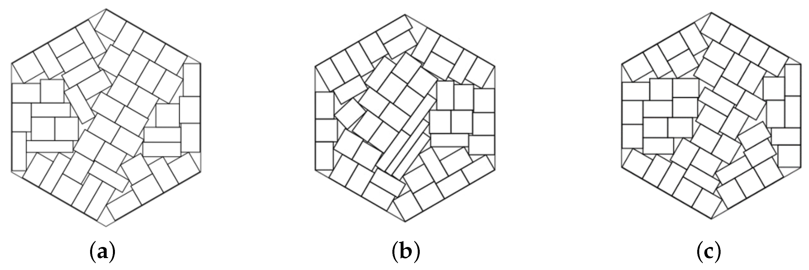
Example 5.

$n=50$, $m=6$, total area of rectangles is 400, hexagonal container.

Figure 11. The best solutions in Example 5: (a) $1\le {\mu }_i\le 2, {\lambda }^{*}=0.32572, f^{*}=90.698\%$; (b) $0.3\le {\mu }_i\le 1.5, {\lambda }^{*}=0.32599, f^{*}=90.548\%$; (c) $0.5\le {\mu }_i\le 2.5, {\lambda }^{*}=0.32498, f^{*}=91.112\%$.

Figure 11. The best solutions in Example 5: (a) $1\le {\mu }_i\le 2, {\lambda }^{*}=0.32572, f^{*}=90.698\%$; (b) $0.3\le {\mu }_i\le 1.5, {\lambda }^{*}=0.32599, f^{*}=90.548\%$; (c) $0.5\le {\mu }_i\le 2.5, {\lambda }^{*}=0.32498, f^{*}=91.112\%$.

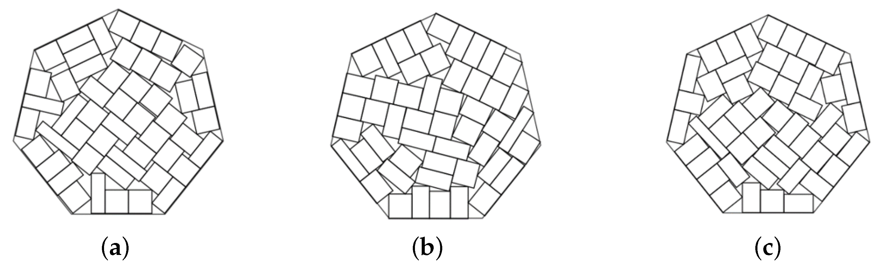
Example 6.

$n=50$, $m=7$, total area of rectangles is 400, heptagonal container.

Figure 12. The best solutions in Example 6: (a) $1\le {\mu }_i\le 2, {\lambda }^{*}=0.322, f^{*}=88.11\%$; (b) $0.5\le {\mu }_i\le 1.5$, ${\lambda }^{*}=0.32, f^{*}=89.22\%$; (c) $0.5\le {\mu }_i\le 2.5, {\lambda }^{*}=0.317, f^{*}=90.92\%$.

Figure 12. The best solutions in Example 6: (a) $1\le {\mu }_i\le 2, {\lambda }^{*}=0.322, f^{*}=88.11\%$; (b) $0.5\le {\mu }_i\le 1.5$, ${\lambda }^{*}=0.32, f^{*}=89.22\%$; (c) $0.5\le {\mu }_i\le 2.5, {\lambda }^{*}=0.317, f^{*}=90.92\%$.

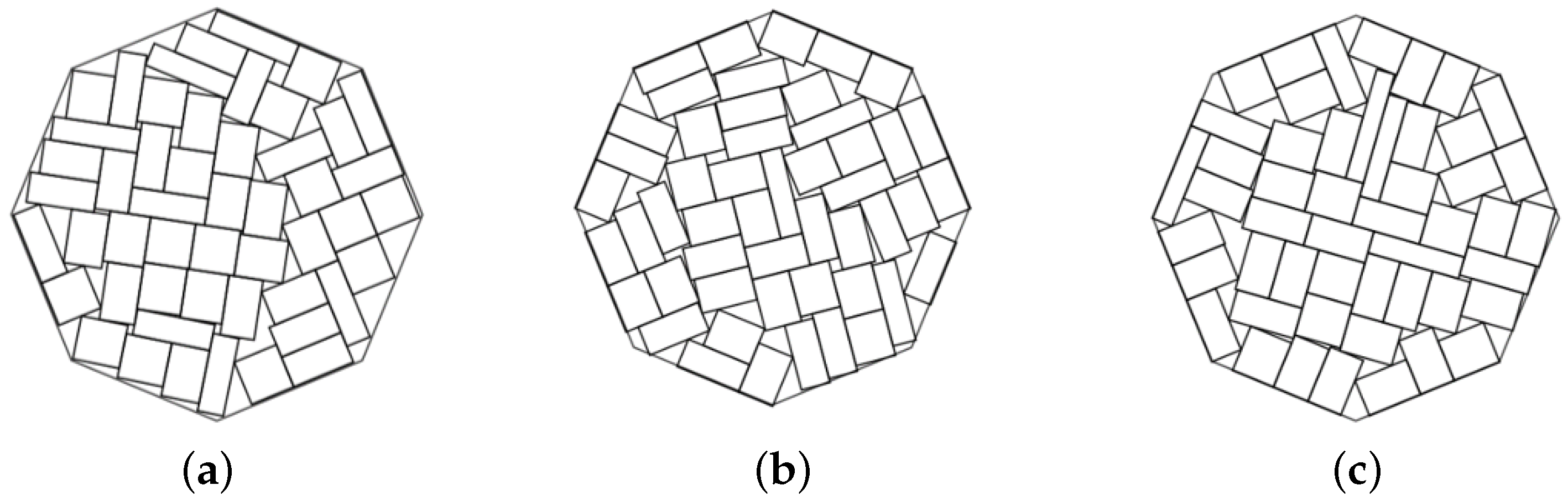
Example 7.

$n=50$, $m=8$, total area of rectangles is 400, octagonal container.

Figure 13. The best solutions in Example 7: (a) $1\le {\mu }_i\le 2, {\lambda }^{*}=0.316, f^{*}=88.51\%$; (b) $0.5\le {\mu }_i\le 1.5$, ${\lambda }^{*}=0.315, f^{*}=89.07\%$; (c) $0.5\le {\mu }_i\le 2.5, {\lambda }^{*}=0.313, f^{*}=90.22\%$.

Figure 13. The best solutions in Example 7: (a) $1\le {\mu }_i\le 2, {\lambda }^{*}=0.316, f^{*}=88.51\%$; (b) $0.5\le {\mu }_i\le 1.5$, ${\lambda }^{*}=0.315, f^{*}=89.07\%$; (c) $0.5\le {\mu }_i\le 2.5, {\lambda }^{*}=0.313, f^{*}=90.22\%$.

5.2. Instances with Prohibited Zones

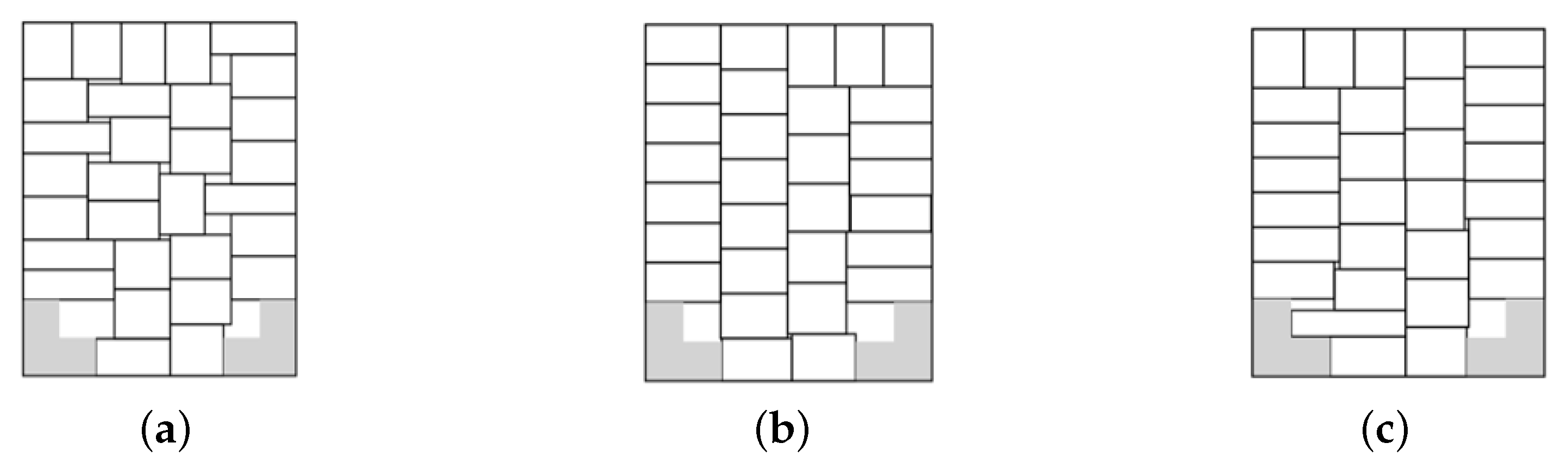
Example 8.

$n=30$, total area of rectangles is 240. Each of the two prohibited zones is a union of two rectangles of area 24. Minimum height rectangular container, $l=15$.

Figure 14. The best solutions in Example 8: (a) $0.8\le {\mu }_i\le 2, h^{*}=18.55, f^{*}=94.4\%$; (b) $0.5\le {\mu }_i\le 1.5$, $h^{*}=18.1, f^{*}=96.98\%$; (c) $0.5\le {\mu }_i\le 2.5, h^{*}=17.87, f^{*}=98.34\%$.

Figure 14. The best solutions in Example 8: (a) $0.8\le {\mu }_i\le 2, h^{*}=18.55, f^{*}=94.4\%$; (b) $0.5\le {\mu }_i\le 1.5$, $h^{*}=18.1, f^{*}=96.98\%$; (c) $0.5\le {\mu }_i\le 2.5, h^{*}=17.87, f^{*}=98.34\%$.

Example 9.

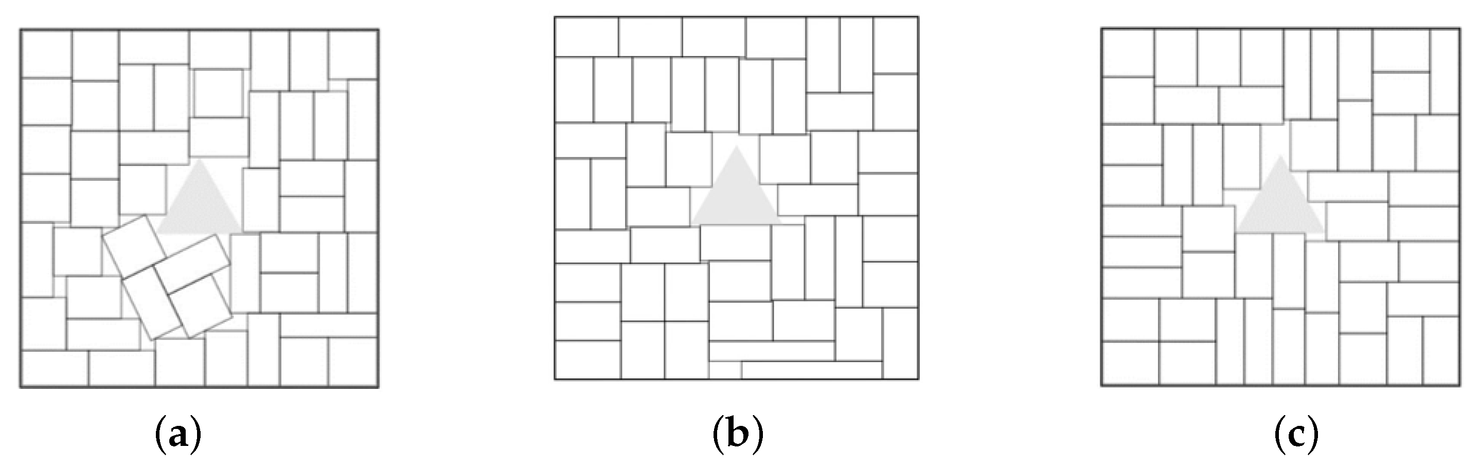
$n=49$, total area of rectangles is 392. Minimal square container, $h=l$. The prohibited zone is a regular triangle of area 11.69.

Figure 15. The best solutions in Example 9: (a) $1\le {\mu }_i\le 2, h^{*}=20.649, f^{*}=94.53\%$; (b) $0.3\le {\mu }_i\le 1.5, h^{*}=20.28, f^{*}=98.1\%$; (c) $0.5\le {\mu }_i\le 2.5, h^{*}=20.263, f^{*}=98.27\%$.

Figure 15. The best solutions in Example 9: (a) $1\le {\mu }_i\le 2, h^{*}=20.649, f^{*}=94.53\%$; (b) $0.3\le {\mu }_i\le 1.5, h^{*}=20.28, f^{*}=98.1\%$; (c) $0.5\le {\mu }_i\le 2.5, h^{*}=20.263, f^{*}=98.27\%$.

Example 10.

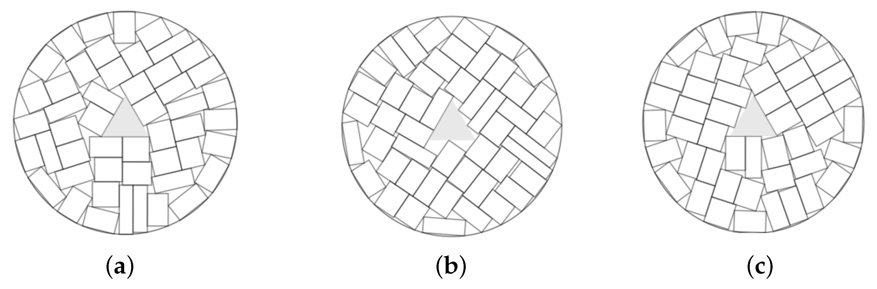
$n=49$, total area of rectangles is 392. Minimal circular container. The prohibited zone is a regular triangle of area 11.69.

Figure 16. The best solutions in Example 10: (a) $1\le {\mu }_i\le 2, r^{*}=12.21, f^{*}=85.88\%$; (b) $0.8\le {\mu }_i\le 2.5, r^{*}=12.05, f^{*}=88.24\%$; (c) $0.5\le {\mu }_i\le 1.5, r^{*}=12.04, f^{*}=88.39\%$.

Figure 16. The best solutions in Example 10: (a) $1\le {\mu }_i\le 2, r^{*}=12.21, f^{*}=85.88\%$; (b) $0.8\le {\mu }_i\le 2.5, r^{*}=12.05, f^{*}=88.24\%$; (c) $0.5\le {\mu }_i\le 1.5, r^{*}=12.04, f^{*}=88.39\%$.

Example 11.

$n=49$, total area of rectangles is 392. Minimal circular container. The prohibited zone is a square of area 16.

Figure 17. The best solutions in Example 11: (a) $1\le {\mu }_i\le 2, r^{*}=12.21, f^{*}=86.7\%$; (b) $0.8\le {\mu }_i\le 2.5$, $r^{*}=12.09, f^{*}=88.49\%$; (c) $0.5\le {\mu }_i\le 1.5, r^{*}=11.98, f^{*}=90.19\%$.

Figure 17. The best solutions in Example 11: (a) $1\le {\mu }_i\le 2, r^{*}=12.21, f^{*}=86.7\%$; (b) $0.8\le {\mu }_i\le 2.5$, $r^{*}=12.09, f^{*}=88.49\%$; (c) $0.5\le {\mu }_i\le 1.5, r^{*}=11.98, f^{*}=90.19\%$.

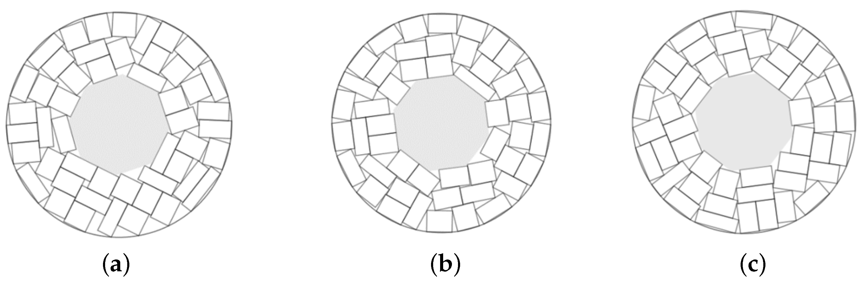
Example 12.

$n=49$, total area of rectangles is 392. Minimal circular container. The prohibited zone is a regular octagon of area 101.82.

Figure 18. The best solutions in Example 12: (a) $1\le {\mu }_i\le 2, r^{*}=13.3, f^{*}=86.42\%$; (b) $0.8\le {\mu }_i\le 2.5$, $r^{*}=13.22, f^{*}=87.71\%$; (c) $0.5\le {\mu }_i\le 1.5, r^{*}=13.21, f^{*}=87.87\%$.

Figure 18. The best solutions in Example 12: (a) $1\le {\mu }_i\le 2, r^{*}=13.3, f^{*}=86.42\%$; (b) $0.8\le {\mu }_i\le 2.5$, $r^{*}=13.22, f^{*}=87.71\%$; (c) $0.5\le {\mu }_i\le 1.5, r^{*}=13.21, f^{*}=87.87\%$.

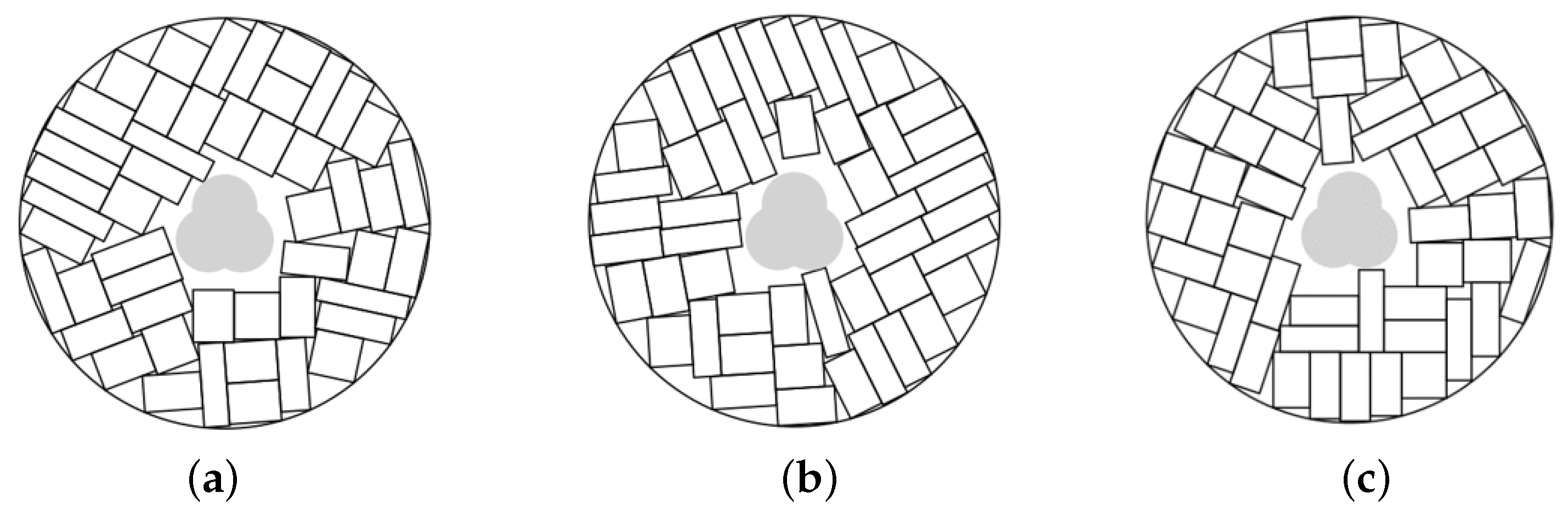
Example 13.

$n=49$, total area of rectangles is 392. Minimal circular container. The prohibited zone is a union of three circles of area 33.17.

Figure 19. The best solutions in Example 13: (a) $1\le {\mu }_i\le 2, r^{*}=12.5305, f^{*}=85.25\%$; (b) $0.8\le {\mu }_i\le 2.5$, $r^{*}=12.5356, f^{*}=85.2\%$; (c) $0.5\le {\mu }_i\le 1.8, r^{*}=12.63, f^{*}=83.81\%$.

Figure 19. The best solutions in Example 13: (a) $1\le {\mu }_i\le 2, r^{*}=12.5305, f^{*}=85.25\%$; (b) $0.8\le {\mu }_i\le 2.5$, $r^{*}=12.5356, f^{*}=85.2\%$; (c) $0.5\le {\mu }_i\le 1.8, r^{*}=12.63, f^{*}=83.81\%$.

Example 14.

$n=46$, total area of rectangles is 368. Minimum scale hexagonal container. The prohibited zone is a union of two rectangles of area 51.2.

Figure 20. The best solutions in Example 14: (a) $1\le {\mu }_i\le 2, {\lambda }^{*}=0.46, f^{*}=84.87\%$; (b) $0.5\le {\mu }_i\le 1.8$, ${\lambda }^{*}=0.449, f^{*}=87.58\%$; (c) $0.3\le {\mu }_i\le 2.5, {\lambda }^{*}=0.446, f^{*}=88.91\%$.

Figure 20. The best solutions in Example 14: (a) $1\le {\mu }_i\le 2, {\lambda }^{*}=0.46, f^{*}=84.87\%$; (b) $0.5\le {\mu }_i\le 1.8$, ${\lambda }^{*}=0.449, f^{*}=87.58\%$; (c) $0.3\le {\mu }_i\le 2.5, {\lambda }^{*}=0.446, f^{*}=88.91\%$.

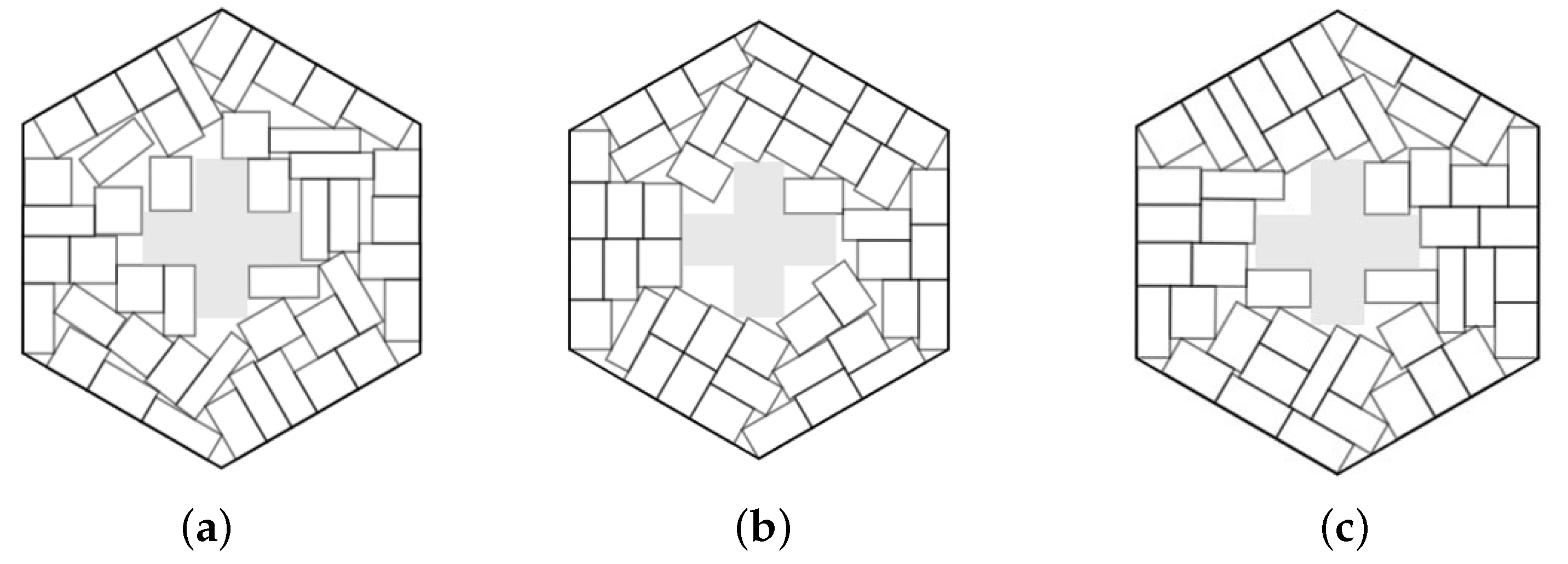
Example 15.

$n=49$, total area of rectangles is 392. Minimum scale hexagonal container. The prohibited zone is a regular hexagon of area 45.25.

Figure 21. The best solutions in Example 15: (a) $1\le {\mu }_i\le 2, {\lambda }^{*}=0.467, f^{*}=84.34\%$; (b) $0.5\le {\mu }_i\le 2.5$, ${\lambda }^{*}=0.4496, f^{*}=91.72\%$; (c) $0.3\le {\mu }_i\le 1.5, {\lambda }^{*}=0.4505, f^{*}=91.31\%$.

Figure 21. The best solutions in Example 15: (a) $1\le {\mu }_i\le 2, {\lambda }^{*}=0.467, f^{*}=84.34\%$; (b) $0.5\le {\mu }_i\le 2.5$, ${\lambda }^{*}=0.4496, f^{*}=91.72\%$; (c) $0.3\le {\mu }_i\le 1.5, {\lambda }^{*}=0.4505, f^{*}=91.31\%$.

6. Conclusions

In this paper, packing soft rectangular objects in an optimized convex container is considered. Each soft rectangle conserves its area; however, dimensions (height, width) can vary in certain limits. Rectangular objects can be freely translated and rotated. The convex container may have (regular or irregular) prohibited zones. The phi-function technique is used to state non-overlapping and containment conditions. The corresponding large-scale nonlinear optimization problem is formulated, and a heuristic is proposed to find reasonable solutions. The principal difference of our model from the earlier research is that rotation of the soft rectangular objects is allowed. Numerical experiments demonstrate that rotation is essential to obtain high-quality arrangements. This is especially important for the case of non-rectangular containers and/or containers with prohibited zones.

A natural generalization of the proposed modeling and solution approach is considering soft irregular objects composed of rectangles, e.g., L- or II-shaped objects. Modeling and solution approaches presented in Section 3 and Section 4 can be used with minor modifications to treat the composed soft rectangular objects. Also, more sophisticated shapes can be considered [25,26,27,28].

In [29], optimized packing of general soft convex polygons was considered. In contrast to the current work, where variables are translation vectors and rotation angles, the variables used in [29] are coordinates of the polygons’ vertices. It would be interesting to specify the approach of [29] for rectangles and compare both models numerically. Results in this direction are on the way.

In many cases a certain minimal distance between the objects must be assured. For example, in land design, land parcels must be accessible from all sides for maintenance and protection. Similarly, a certain distance between the land parcels must be guaranteed if they are used for contaminating activities. Correspondingly, the parcels must be sufficiently separated. This gives rise to the so-called sparse or sparsest packing problem [30]. An interesting direction for future research is to consider sparse formulations for packing soft rectangles.

Considering 3D soft rectangles (cuboids) is also a promising area for future research. The main model (8)–(13) and the heuristic are dimension-independent and thus can be applied directly for the 3D case. Convex 3D containers of simple forms (cuboid, sphere, prism) also do not require significant changes in the main model. Reference [31] is included in Appendix A. Optimized packing of soft cuboids can also be applied to transportation problems [32].

Solutions obtained by the proposed heuristic can be used as starting points either in other heuristics (see, e.g., ref. [33] and the references therein) or in global optimization techniques [34].

One of the interesting directions of future research is the application of our methodology to solving coverage [35,36,37] and partition problems [38].