Memetic-Based Biogeography Optimization Model for the Optimal Design of Mechanical Systems

Abstract

The science of biogeography was described through mathematical equations in 1967 by Robert MacArthur and Edward Wilson. In 2008, Dan Simon presented an algorithm called biogeography-based optimization, or BBO, which used some of the principles and definitions described in MacArthur and Wilson’s book. The objectives of this work were to study the behavior of the BBO method when it is hybridized with other evolutionary search methods and to analyze the effect of its application to some examples of mechanical engineering systems. The operators considered in the hybridization study are genetic recombination (crossover) and local search, aiming to overcome the limitations and difficulties that arise when using the original BBO. The results of the original BBO were promising in the context of a global search. However, there is a diversity problem that does not allow for good quality increments in the final phase of the evolutionary process. The additional modifications included, such as the concept of blending in migration, the cycle of mutations and the replacement of the worst solutions by injection of new ones, all show positive effects on the method’s performance. However, the biggest increase happened with the implementation of the hybridization processes. Crossover improved the speed and diversity of the population in some cases, while local search helped the algorithm in later generations, allowing it to quickly reach the optimum point. With this mentioned, it is important to note that the best results were all obtained with the fully modified algorithm. Statistical tests were implemented to validate the significance of changes due to modifications included in the original proposal of BBO.

1. Introduction

Engineering problems have become increasingly complex, making their analytical resolution practically impossible to complete in many situations. Numerical solution methods have, therefore, been given greater focus. Optimization, which fits into this category, has become one of the most pivotal subjects in the day-to-day of a modern engineer specifically because there is not an area in engineering where optimization is not involved in some way. The optimal design of engineering systems has, therefore, undergone many important developments in recent years. One of the biggest developments was the introduction of the genetic algorithm (GA) by John Holand [1], the first evolutionary algorithm with structured operators, which is an event that revolutionized the entire optimization environment. Since then, the scientific community has been perfecting this method, creating a large number of proposals for new operators based on all kinds of schemes and heuristics, all to solve optimization problems. The genetic algorithm uses some ideas from other scientific fields, such as genetics and biology, and applies them mathematically, in the form of an algorithm, to different areas of engineering. There are also other methods inspired by other areas, such as memetic algorithms (MAs), which are based on biology (genetic evolution) [2] and learning processes (cultural evolution) [3,4], and the algorithm that will be presented in this article, biogeography-based optimization.

Biogeography is the study of the distribution of species and ecosystems in geographical space over geological time. Biogeographical research combines information and ideas from different fields, from the physiological and ecological constraints on the spreading of organisms to the geological and climatological phenomena that occur on a global scale in evolutionary periods.

Biogeography-based optimization is an evolutionary algorithm (EA), introduced in 2008 by Dan Simon [5,6], that optimizes a function by iteratively and stochastically improving its solutions according to a quality measure or fitness function. Typically, this method is used to study multivariate problems, and since it does not require the calculation of a gradient function, it can also be used to optimize discontinuous functions. BBO optimizes a problem by maintaining a population of candidate solutions and creating new solutions through the migration process. At the end of the article, Simon presented a list of points for improvement, which created a wave of innovation and research focused on the BBO method.

Ma [7] started off by introducing novel linear and non-linear migration methods, allowing the algorithm to improve in some characteristics, mainly related to the convergence speed. Ma, together with Simon [8], added a variation in the migration processes named blending, trying to increase the population diversity by mixing the features of good and bad solutions instead of completely replacing the worst solutions. Boussaïd et al. [9] tried to solve one of the topics to improve by implementing three variations of BBO for constrained optimization (CBBO); all of them presented different methods to deal with solutions that violated the constraints. Bi and Wang [10] proposed another variation of BBO for constrained optimization, called ε-BBO, inspired by the penalty method, which also used a dynamic migration procedure. There were also other authors, like Ma et al. [11], Bi et al. [12] and Xu [13], who modified BBO to be used in multi-objective problems.

In addition to modifications to the BBO method, some authors have used BBO together with other optimization techniques and methods in a hybridization process. Kundra and Sod [14] used a hybrid BBO and PSO method to solve Cross-County Path discovery. Albrase et al. [15] used a BBO hybrid with linear programming to solve directional over-current relays examples. In terms of population-based hybrids, the most common method is the Differential Evolution (DE) method [16,17,18], and the results showed that this hybrid showed improvements when compared to the BBO or DE methods. Other commonly hybridized methods are Case Base Reasoning (CBR) [19], Simplex Algorithm [20], Artificial Bee Colony Algorithm [21] and Harmony Search [22]. Zhao et al. [23] also proposed a binary BBO algorithm that uses the standard BBO migration and two new mutation operators based on binary recombination.

This work will expose the BBO algorithm to four problems of different complexity, aiming to study its behavior and modify it to overcome its weaknesses, such as poor local search and low convergence speed. To do this, not only were modifications introduced to the algorithm presented in the literature, but also other concepts from the world of optimization, such as crossover, local optimizer, and replacement of the worst solutions, were used [24,25].

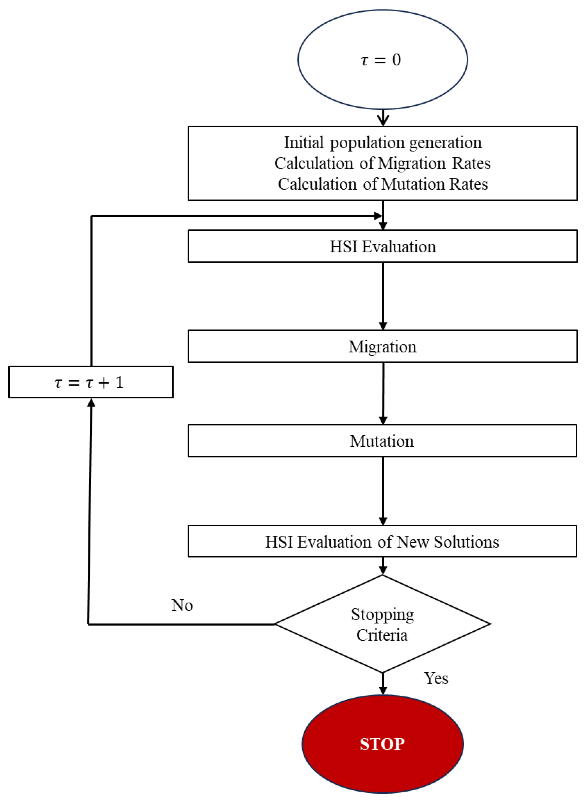
2. BBO Approach Model

The science of biogeography, created in the 19th century, was considered to be descriptive and historical, but in 1967, Robert MacArthur and Edward Wilson published The Theory of Island Biogeography [26], where they tried to describe this phenomenon in mathematical equations. These models have tried to describe how species move from one island to another, how new species appear, and how they become extinct. In this case, the term “island” should not be taken at face value but as a place that is geographically isolated from other habitats. Therefore, the term “habitat” should be used to better describe these locations.

Sites with good life retention characteristics are associated with habitats with a high habitat suitability index (HSI). Factors such as the presence of drinking water, which are related to the HSI, are referred to as suitability index variables (SIVs). In mathematical terms, the SIV can be called the independent variables and the HSI the dependent variables. Then, the habitats with high HSI will have a lot of species, while the habitats with low HSI will have fewer species. In real life, the emigration of a species may not lead to its extinction, but in this case, the emigration of a species will lead to the extinction of the species in that habitat. Low HSI habitats will have a high immigration rate due to their smaller population numbers and non-competitive environment. On the contrary, high HSI habitats will have a high emigration and low immigration rate.

Good solutions are associated with habitats with high HSI, while habitats with low HSI are associated with bad solutions. Solutions with high HSI are more resistant to change, so solutions with high HSI tend to share characteristics with low HSI solutions. The diversity of individuals is related to HSI, so when an individual arrives in a habitat with low HSI, the habitat’s HSI tends to increase. This approach has been given the name biogeography-based optimization (BBO), which was created and presented by Dan Simon [5]. Figure 1 presents the flow diagram of the method.

2.1. Mathematical Model

Figure 2 shows a model of the abundance of species in a single habitat. The emigration rate $\mu$ and the immigration rate $\lambda$ are functions of the number of species in the habitat. Looking at the immigration curve, it is possible to note that its maximum will occur when the migration rate of the habitat is $I$, which happens when the number of species of the habitat reaches zero. As the number of species increases, the immigration process will become more competitive, which will lead to a decrease in the number of species able to complete the process, resulting in a reduction in the immigration rate. The maximum number of species present in a habitat is defined as $S_{\max }$, at which point the immigration rate will be zero. The emigration curve, on the other hand, will have its maximum $E$ when the population of the habitat reaches its maximum and will be zero when there are no more species in the habitat.

The equilibrium point, $k_0$, is obtained when the rates of emigration and immigration are equal. This point can occasionally differ due to temporary effects, such as diseases. Figure 2 represents both rates as straight lines, but in reality, they can be complex curves. However, this representation is a good approximation of the migration process.

Now let’s consider a probability $P_s$ that the habitat contains exactly $S$ species. The probability changes with time, from $t$ to $t+\mathsf{\Delta }t$, following the equation below;

$$P_s\left(t+\mathsf{\Delta }t\right)=P_s\left(t\right)\left(1-\lambda \mathsf{\Delta }t-{\mu }_s\mathsf{\Delta }t\right)+P_{s-1}{\lambda }_{s-1}\mathsf{\Delta }t+P_{s+1}{\mu }_{t+1}\mathsf{\Delta }t,$$

(1)

where ${\lambda }_s$ and ${\mu }_s$ are the immigration and emigration rates when there are $S$ species in the habitat.

Assuming that the time interval $\mathsf{\Delta }t$ is small enough, the probability of more than one emigration or immigration can be ignored. Using a limit in the above equation, with the time interval tending to zero, the following equation emerges:

$${\dot{P}}_s=\left\{\begin{array}{c}-\left({\lambda }_s+{\mu }_s\right)P_s+{\mu }_{s+1}{P}_{s+1}, S=0\\ -\left({\lambda }_s+{\mu }_s\right)P_s+{\lambda }_{s-1}{P}_{s-1}+{\mu }_{s+1}{P}_{s+1}, 1<S\le S_{\max }-1\\ -\left({\lambda }_s+{\mu }_s\right)P_s+{\lambda }_{s-1}{P}_{s-1}, S=S_{\max }\end{array}\right.$$

(2)

Aiming to simplify the notation, Simon [5] decided to perform the following changes: $n=S_{\max }$ and $P={\left[P_0\dots P_n\right]}^T$. Then, it is possible to write the previous equation as follows:

$$\dot{P}=AP,$$

(3)

where the $A$ matrix is given by the following:

$$A=\left[\begin{array}{ccccc}-\left({\lambda }_0+{\mu }_0\right)& {\mu }_1& 0& \dots & 0\\ {\lambda }_0& -\left({\lambda }_1+{\mu }_1\right)& {\mu }_2& \ddots & ⋮\\ ⋮& \ddots & \ddots & \ddots & ⋮\\ ⋮& \ddots & {\lambda }_{n-2}& -\left({\lambda }_{n-1}+{\mu }_{n-1}\right)& {\mu }_n\\ 0& \dots & 0& {\lambda }_{n-1}& -\left({\lambda }_n+{\mu }_n\right)\end{array}\right]$$

(4)

Considering the lines from Figure 2, the migration rates can be described as follows:

$${\mu }_s={\displaystyle \frac{Es}{n}}$$

(5)

$${\lambda }_s=I\left(1-{\displaystyle \frac{s}{n}}\right)$$

(6)

The equations above can be presented in a different form if the number of species is replaced by the value calculated in the fitness function [27]:

$${\lambda }_i=I{\displaystyle \frac{f_{\max }-f\left(H_i\right)+\epsilon }{f_{\max }-f_{\min }+\epsilon }},$$

(7)

$${\mu }_i=E{\displaystyle \frac{f\left(H_i\right)-f_{\min }+\epsilon }{f_{\max }-f_{\min }+\epsilon }},$$

(8)

where $H_i$ represents the solution in the study.

Following the same ideas, the calculation of the migration rates can also be given by the ranking of the solutions after they have been placed in descending order as follows [27]:

$${\lambda }_i=I{\displaystyle \frac{i}{n}}$$

(9)

$${\mu }_i=E\left(1-{\displaystyle \frac{i}{n}}\right)$$

(10)

Now, considering the case where $E=I$, we have the following:

$${\lambda }_s+{\mu }_s=E=I,$$

(11)

and the matrix A transforms into the following:

$$A=E\left[\begin{array}{ccccc}-1& {\displaystyle \frac{1}{n}}& 0& \dots & 0\\ {\displaystyle \frac{n}{n}}& -1& {\displaystyle \frac{2}{n}}& \ddots & ⋮\\ ⋮& \ddots & \ddots & \ddots & ⋮\\ ⋮& \ddots & {\displaystyle \frac{2}{n}}& -1& {\displaystyle \frac{n}{n}}\\ 0& \dots & 0& {\displaystyle \frac{1}{n}}& -1\end{array}\right]={EA}^{\prime }$$

(12)

It is possible to note that zero is an eigenvalue of matrix $A^{\prime }$ with the corresponding eigenvectors:

$$v=\left[v_1\dots v_{n+1}\right]$$

(13)

$$v_i=\left\{\begin{array}{c}{\displaystyle \frac{n!}{\left(n-1-i\right)!\left(i-1\right)!}}, (i=1,\dots ,i^{\prime })\\ v_{n+2-i}, \left(i=i^{\prime }+1,\dots ,n+1\right)\end{array}\right.$$

(14)

The value, in steady state, of the probability of the number of each species is given by the following:

$$P\left(\infty \right)={\displaystyle \frac{v}{{\sum }_{i=1}^{n+1}{v}_i}}$$

(15)

The computation of the probability, which depends on the migration rates, is previously calculated, as shown in Equation (16). This formulation solves a problem that restricts the number of possible initial solutions.

$$P_i=\left\{\begin{array}{c}{P}_0={\displaystyle \frac{1}{1+{\sum }_{k=1}^n\frac{{\lambda }_0{\lambda }_1\dots {\lambda }_{k-1}}{{\mu }_1{\mu }_2\dots {\mu }_k}}}, i=0\\ P_i={\displaystyle \frac{{\lambda }_0{\lambda }_1\dots {\lambda }_{i-1} }{{\mu }_1{\mu }_2\dots {\mu }_i\left(1+{\sum }_{k=1}^n\frac{{\lambda }_0{\lambda }_1\dots {\lambda }_{k-1}}{{\mu }_1{\mu }_2\dots {\mu }_k}\right)}}, 1\le i\le n \end{array}\right.$$

(16)

Simon [5] recommends the use of $E=I=1$, $N=50$ and $m_{\max }=0.01$ as the initial parameters for the method.

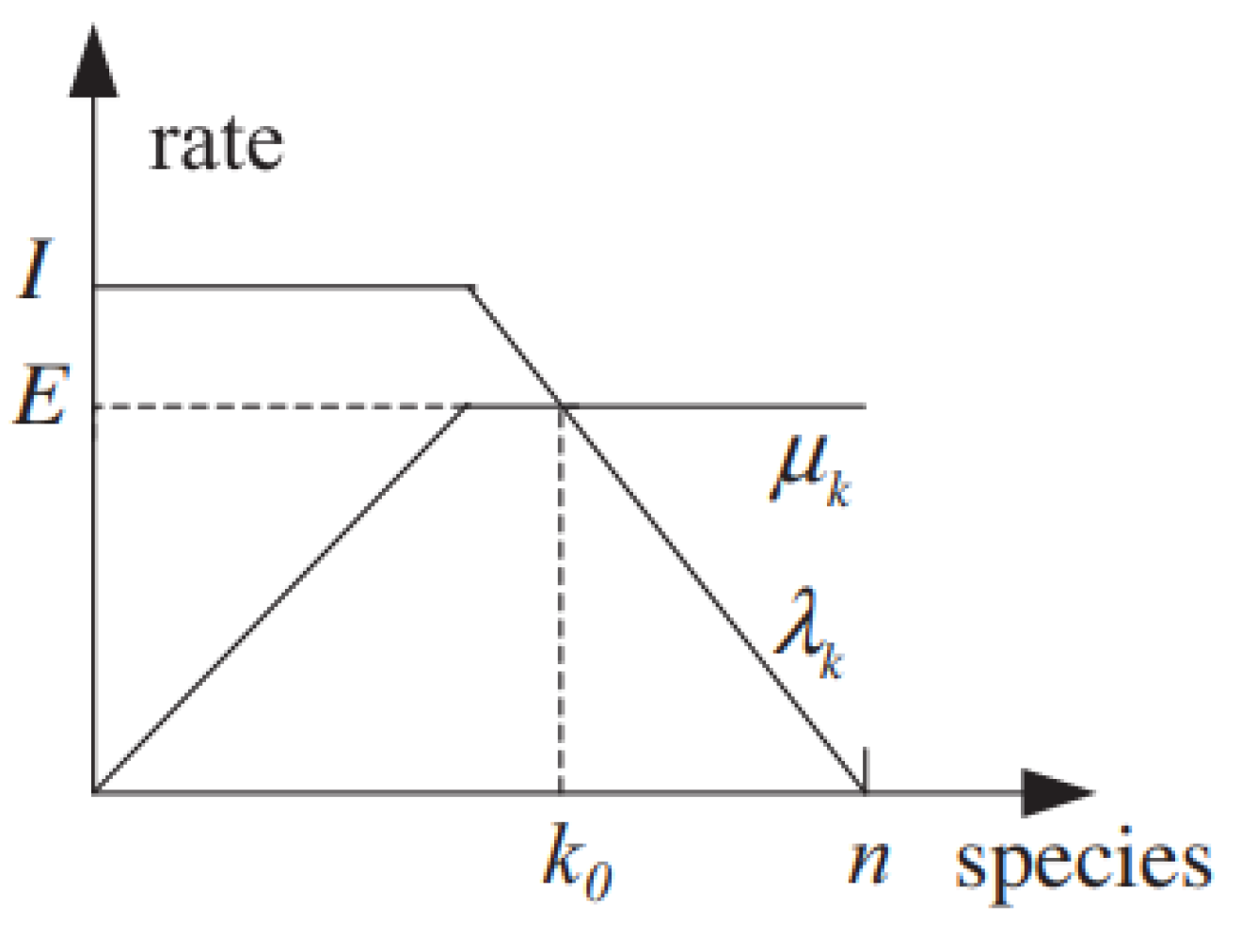
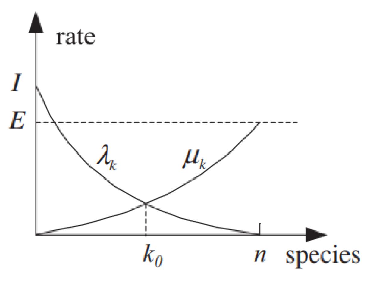
2.2. Migration Operator

Supposing that the population of solutions can be represented as a vector of integers, each of the numbers is considered a SIV. The HSI, which is analogous to GA fitness, can be used in other processes of optimization based on populations. High HSI solutions represent the habitats with several species, and low HSI solutions represent the habitats with fewer solutions. It is possible to assume that each solution has an identical migration curve (with $E=I$), but the value of $S$ represented by the solution remains dependent only on its HSI.

The migration rates of each solution are used to probabilistically share information between habitats. The immigration rate is, therefore, used to determine whether the SIV of each solution will change. If in a given solution $S_i$, an SIV is randomly selected to be modified, then the emigration rate of the other solutions will decide from which of the solutions an SIV located in the same position will migrate to solution $S_i$. This process is quite similar to other reproduction processes from GAs, but this method differs from them in a very important aspect. In the GA, reproduction by recombination is used to create new solutions, while BBO migration is used to modify existing solutions. It is, therefore, possible to say that, unlike the reproduction process of the GA, the migration of the BBO is an adaptive process. In algorithmic terms, the migration operator can be described in the following way (Algorithm 1):

Algorithm 1: Migration’s Pseudocode
1	For  $d=1$  to  $D$  do
2	If  $\mathrm{rand} < {\lambda }_i$  then
3	$\mathrm{Select} \mathrm{another} \mathrm{habitat} (H_j$$) \mathrm{with} \mathrm{a} \mathrm{probability} \propto {\mu }_j$
4	Define $H_i\left(d\right)=H_j\left(d\right)$
5	End If
6	End For

where $d$ represents the variable under study, and $D$ represents the size of the problem.

Normally, the use of linear models (Figure 2 and Equations (5)–(10)) to describe the migration curves is sufficient, but there are also other different options to describe this operator. Ma [7] presented several other options for the migration operator, such as the trapezoidal model. As described in the following equation and represented graphically in Figure 3,

$${\lambda }_s=\left\{\begin{array}{c}I, s\le i^{\prime }\\ 2I\left(1-{\displaystyle \frac{s}{n}}\right), i^{\prime }<s\le n\end{array}\right.,$$

(17)

$${\mu }_s=\left\{\begin{array}{c}2\cdot {\displaystyle \frac{E}{n}}, s\le i^{\prime }\\ E, i^{\prime }<s\le n\end{array}\right.,$$

(18)

where $i^{\prime }$ is the smallest integer close to $\left(n+1\right)/2$.

Ma [7] also presented some non-linear models, such as the quadratic (Equations (19) and (20), and Figure 4) and sinusoidal (Equations (21) and (22), and Figure 5) models. These models aim to provide a more accurate simulation of real-life migration patterns by incorporating non-linearities.

$${\lambda }_s=I{\left(1-{\displaystyle \frac{s}{n}}\right)}^2$$

(19)

$${\mu }_s=E{\left({\displaystyle \frac{s}{n}}\right)}^2$$

(20)

$${\lambda }_s={\displaystyle \frac{I}{2}}\left(\cos \left({\displaystyle \frac{s\pi }{n}}\right)+1\right)$$

(21)

$${\mu }_s={\displaystyle \frac{E}{2}}\left(-\cos \left({\displaystyle \frac{s\pi }{n}}\right)+1\right)$$

(22)

Migration, being one of the main points of interest in the method, has been severely modified and improved. Mainly, Ma and Simon [8] presented a new hybrid algorithm called Blended BBO (B-BBO) that uses some ideas from GAs’ crossover operators, creating a migration operator that mixes each component of an immigrating solution ($H_i$) with the corresponding component of the emigrating solution ($H_j$), as follows:

$$H_i^{\prime }\left(d\right)=\alpha H_i\left(d\right)+\left(1-\alpha \right)H_j\left(d\right),$$

(23)

where $\alpha$ is a number between $\left[0, 1\right]$, which can be a predetermined or random value.

With the standard migration operator, it is possible to improve poor solutions by using the features of the best solutions. However, the blending operator makes it possible not only to do this, but also to avoid the degradation of good solutions, since they retain some of their original properties. This operator also allows for the creation of new components, promoting population diversity.

2.3. Mutation Operator

Cataclysmic events can drastically change the HSI of a natural habitat, which can make it so that the number of species varies from the equilibrium point $k_0$ with a mutation of SIV. Each element of the population has an associated probability, which indicates the probability of expecting a priori that there is a solution to the problem in question. Solutions with a very low or very high HSI are equally unlikely to mutate, and solutions with a medium HSI are relatively likely. If a solution $S$ has a low probability $P_i$, then the probability of it being mutated is high. On the other hand, a solution with a high probability will have fewer opportunities to mutate. This can be implemented using the following formula:

$$m_i=m_{\max }\left({\displaystyle \frac{1-P_i}{P_{\max }}}\right),$$

(24)

where $m_{\max }$ is a parameter defined by the user that represents the maximum mutation rate, and $P_{\max }$ is the maximum of $P_i$ in the population

This method makes it possible to improve solutions with low HSI. Furthermore, with the use of elitism, which guarantees that the best solutions are kept in the study space, mutation adds some guarantee that the algorithm will not get stuck in a local optimum. Algorithmically, this process can be described as shown in the pseudocode below (Algorithm 2), with $u_d$ and $l_d$ representing the upper and lower bounds of the variable, respectively.

Algorithm 2: Pseudocode for BBO’s standard mutation
1	For  $d=1$  to  $D$  do
2	If  $\mathrm{rand}<m_i$  then
3	$\mathrm{Define} H_i\left(d\right)=l_d+\mathrm{rand}\cdot \left(u_d-l_d\right)$
4	End If
5	End For

Recently, the mutation process has been simplified so that only habitats with low HSI can be mutated, eliminating the need to calculate the species count probability and mutation rate for each species. Like migration, the mutation operator has undergone several modifications. Hao’s taxonomic mutation [28] is one of these modifications. With this operator, solutions with a high HSI are excluded from the process, and the type of mutation differs depending on whether the HSI of the solutions is medium or low. For medium HSI solutions, since the solution is somewhat valuable, a differential mutation process will be used, using a $P_C$ crossover rate to judge how the solution will be mutated. For the solutions with low HIS, a random mutation similar to BBO’s standard mutation will be used, but instead of using the problem bounds ($u_d$ and $l_d$) it will use the population’s best and worst solutions. For solutions with low HSI, a random mutation will be used, similar to the standard BBO mutation, but instead of using the problem limits ($u_d$ and $l_d$), it will use the best and worst solutions in the population. The following algorithm (Algorithm 3) represents the pseudocode for the differential mutation.

Algorithm 3: Pseudocode for differential mutation
1	For $i=1$ to $N_{\mathrm{pop}}$ do
2	$\mathrm{Select} \mathrm{three} \mathrm{solutions} (H_1, H_2, H_3$) and a dimension ($d_r$) randomly
3	$\mathbf{For} d=1$ to $D$ do
4	If  $\mathrm{rand}<m_i$  then
5	If  $\mathrm{rand}\le P_C$ or $d==d_r$ then
6	$H_i\left(d\right)=H_1\left(d\right)+F\cdot \left(H_2\left(d\right)-H_3\left(d\right)\right)$
7	Else
8	$H_i\left(d\right)=H_{\min }\left(d\right)+\mathrm{rand}\cdot (H_{\max }\left(d\right)-H_{\min }\left(d\right)$
9	End If
10	Else
11	If  $\mathrm{rand}\le P_C$ or $d==d_r$ then
12	$H_i\left(d\right)=H_1\left(d\right)$
13	Else
14	$H_i\left(d\right)=H_{\mathrm{best}}\left(d\right)+F\cdot \left(H_2\left(d\right)-H_3\left(d\right)\right)$
15	End If
16	End If
17	End For
18	End For

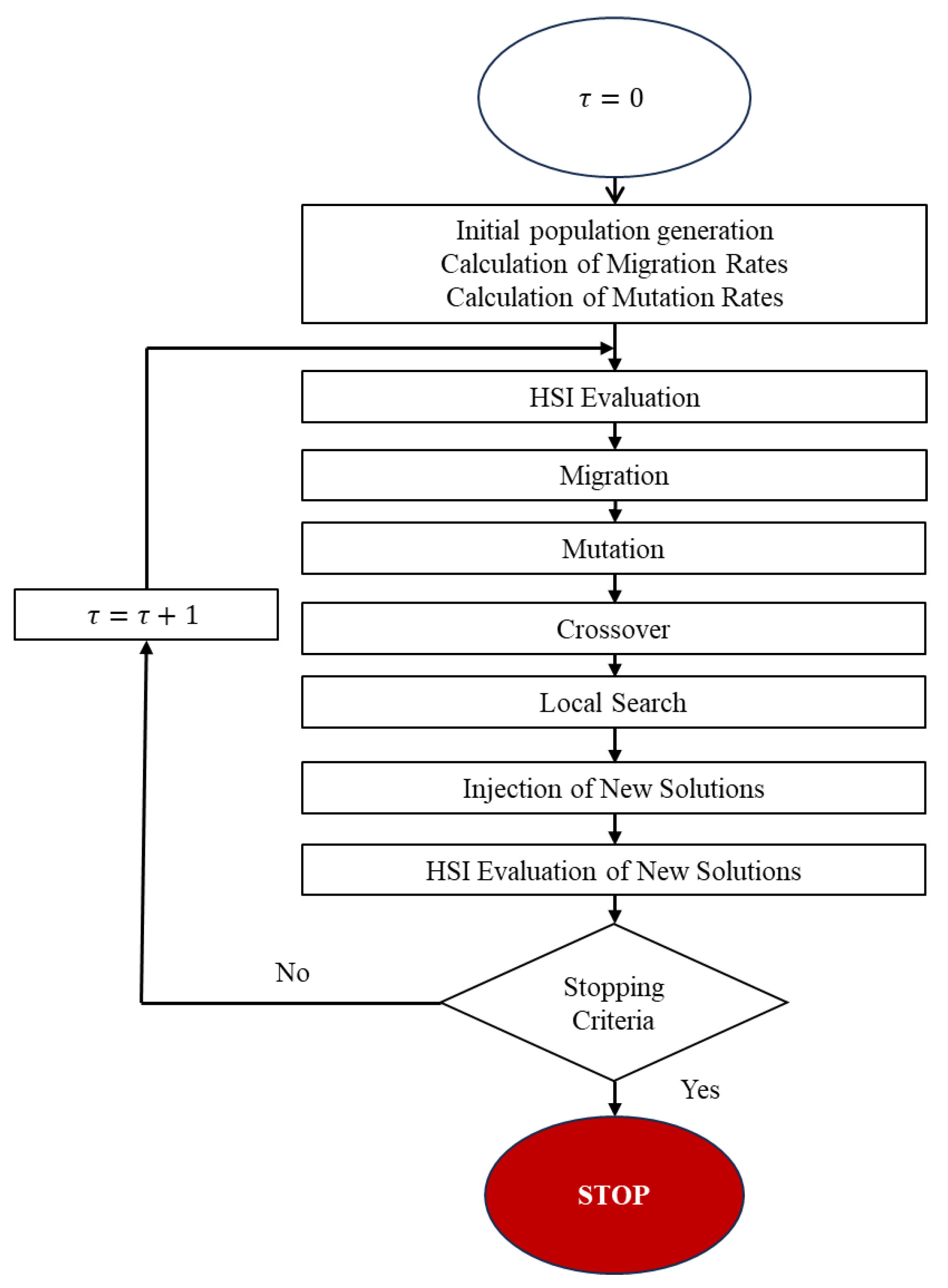
3. Proposed Approach for BBO

3.1. Operators, Modifications, and Hybridization

Initially, only the concepts presented by Dan Simon [5], such as the linear migration model and basic mutation, were used in some very basic example functions to carry out an initial study of the method. Later, the migration models presented here by Ma [7], the taxonomic mutation operator by Hao [28], and the concept of blending in migration by Ma and Simon [8] were added. This completed the initial standard BBO algorithm, which was then applied to the first three cases presented below, allowing the algorithm’s behavior to be studied further.

Once this phase had been completed, the algorithm was modified to be able to remedy some of its shortcomings. To do this, a mutation cycle, in which the mutation operators are used several times in the same generation, only allows for the addition of improved solutions. A solution injection process was also added, where the last 10% of the population was replaced by new solutions at the end of each generation. All these processes were added in an initial iteration of the studies to improve the diversity of the algorithm’s population.

Finally, in the hybridization section, two concepts from the genetic and memetic algorithms were implemented to improve the method’s performance. Initially, binary crossover operators were added to improve the exchange of genetic information, something that had already been explored in the BBO world with the concept of blending [8]. For the implementation of these operators, it was also necessary to implement a binary decoder and encoder since most of the operators and heuristics of the BBO method are in the real domain. Recombination processes are based on the selection of a couple for each child that will be generated. Three operators, the single-point crossover (SP) [29], the multi-point crossover (MP) [29], and the uniform crossover (U) [30], were subjected to two different mating selection mechanisms (MSMs).

The first strategy for MSM, denoted by Previous Elites-based Selection (PEbS), is proceeded as follows:

The first parent is selected from the current population with a probability equal to the migration rate (proportional to rank position). The second parent is selected randomly from the best solutions stored in previous generations. Then, the offspring created by crossover will be evaluated. The new population will be composed using the best solutions from the current population and the offspring. The enlarged population is sorted by fitness, and the worst individuals are eliminated to restore the original size of the population.

The second strategy for MSM, denoted by Independent Selection-based Fitness (ISbF), is performed as follows:

The current population is divided into two groups according to the fitness of each solution: the best (elite) group and the worst group of solutions [25]. Each group provides a parent, which is selected through a roulette method (Equation (25)). The two stochastic procedures are independent. Then, the offspring created will all be placed in the population, replacing every solution not belonging to the elite:

$$P\left({\mathit{x}}_j^k\right)={\displaystyle \frac{f\left({\mathit{x}}_{\mathit{j}}^{\mathit{k}}\right)}{{\sum }_{j=1}^{N_{\mathrm{pop}}}f\left({\mathit{x}}_j^k\right)}},$$

(25)

where $f\left({\mathit{x}}_{\mathit{j}}^{\mathit{k}}\right)$ represents the fitness value of the solution and $N_{\mathrm{pop}}$ the size of the population.

To conclude the hybridization, it was also added a Hooke–Jeeves algorithm as a search optimizer to improve the final generations’ local search, something that has been well documented as a flaw of the BBO method. This operator will allow for an improvement of the search velocity, allowing for the algorithm to reach the end solution with greater ease. The Hooke–Jeeves method is common in the world of optimization since it allows for an efficient search for spaces of great dimensions, even if the objective function is very complex. This method and its parameters were altered so that its performance and synergy with the other operators were greatly improved. The following algorithm (Algorithm 4) shows the pseudocode for the local search method.

Algorithm 4: Hook-Jeeves local search method pseudocode
1	$\mathrm{Compute} \mathrm{the} \mathrm{step} \mathrm{size} (h^1$)
2	For $i=1$ to $N_{\mathrm{pop}}$ do
3	$\mathrm{Select} \mathrm{point} \left(\mathrm{solution}\right) \mathrm{to} \mathrm{be} \mathrm{explored}, H_i$
4	Perform the first step iteration (Equation (26))
5	$\mathrm{Evaluate} \mathrm{the} \mathrm{new} \mathrm{solution}, H_{\mathrm{new}}$ in BBO algorithm
6	$\mathbf{If} H_{\mathrm{new}}$ is better than $H_i$ then
7	$H_i$$\leftarrow H_{\mathrm{new}}$
8	End If
9	Save the solution information, $H_{\mathrm{old}}$
10	/* Local search loop */
11	While stopping criteria are not verified do
12	Compute the new step value (Equation (27))
13	Compute the new solution $H_{\mathrm{new}}$
14	If $H_{\mathrm{new}}$ is better than $H_{\mathrm{old}}$ then
15	$H_{\mathrm{old}}\leftarrow H_{\mathrm{new}}$
16	If $H_{\mathrm{new}}$ better than $H_i$ then
17	$H_i\leftarrow H_{\mathrm{new}}$
18	End If
19	End If
20	End While
21	End For

The first step, $h^1$, is calculated as follows:

$$h^1\left(j\right)=H_1\left(j\right)-H_{N_{\mathrm{pop}}}\left(j\right),$$

(26)

where $j$ represents the dimension, $H_1$ is the best solution from current population, and $H_{N_{\mathrm{pop}}}$ is the worst solution. The step reduction is given by the following:

$$h^i\left(j\right)=\left({\displaystyle \frac{1}{i}}\right)\cdot h^1\left(j\right),$$

(27)

where $i$ represents the number of cycles of the local search loop. It is important to mention that the steps are subtracted and added so that a complete search can be carried out.

For the practical cases presented here, the algorithm was tested using the migration operator in the standard and blending versions and using the mutation operator in the standard and taxonomic versions. These operators were then tested with a local optimizer and a crossover operator. First, each approach was conducted separately and after using a hybrid procedure. The studies focused on the best solutions obtained and the evolution of the elite average over the generations.

3.2. Numerical Implementation

The algorithm was implemented in FORTRAN with the intel compiler for visual studio. Initially, the algorithm randomly creates the initial population and calculates the mutation and migration rates. After that, the algorithm will evaluate the solutions and rank them according to their fitness. Then, the solutions will go through the migration process, where it was defined that the top two solutions will not receive information from other solutions but only share. Next, the algorithm moves on to the mutation operators, where all solutions can be mutated, but due to the mutation cycle, the newly generated solutions will only enter the population if they represent an improvement. For each one hundred generations, the solutions will be subjected to crossover operators. After this procedure, the algorithm enters the local search phase. Here, the new population is classified so that at the end of this phase, the solution injection process can replace the worst solutions. Figure 6 shows the flow diagram of the hybridized algorithm.

In terms of simulation parameters, it used 50 initial solutions, 10% of which represent the evaluated elite, emigration ($E$), and immigration ($I$) values equal to one, a maximum mutation ($m_{\max }$) of 0.01, and an initial number of mutation cycles of three, increased by one after every 100 generations, until to maximum value of 20.

For the Hook–Jeeves local search, a constant selection probability equal to 0.1 was used to select solutions from the BBO population, except for the two best solutions, which were always selected. The stopping criteria of the Hook–Jeeves local search is based on the number of cycles set at one hundred.

4. Case Studies

4.1. Case Study 1: Welded Beam Design

The welded beam, as shown in Figure 7, is a classical optimization problem collected from [32], where its objective is to minimize the cost of the welded joint. This is a non-linear problem, not only in its objective function but also in its constraints.

From a geometrical standpoint, the objective function can be given as follows:

$$f\left(x_1,x_2,x_3,x_4\right)=\left(C_1+C_3\right)\cdot V_{welding}+C_2\cdot V_{\mathrm{beam}},$$

(28)

where $\left(x_1,x_2,x_3,x_4\right)=\left(h,l,t,b\right)$ and where $C_1=0.10471,C_2=0.04811,C_3=1$, and,

$$V_{\mathrm{welding}}=x_1^2\cdot x_2$$

(29)

$$V_{beam}=x_3\cdot x_4$$

(30)

The constraints imposed in the problem are the following:

$$g_1\left(\mathit{x}\right)=\tau \left(\mathit{x}\right)-{\tau }_{\max }\le 0,$$

(31)

$$g_2\left(\mathit{x}\right)=\sigma \left(\mathit{x}\right)-{\sigma }_{\max }\le 0,$$

(32)

$$g_3\left(\mathit{x}\right)=x_1-x_4,$$

(33)

$$g_4\left(\mathit{x}\right)=C_1\cdot x_1^2+C_2\cdot x_3\cdot x_4\cdot \left(L+x_2\right)-5\le 0,$$

(34)

$$g_5\left(\mathit{x}\right)=0.125-x_1\le 0,$$

(35)

$$g_6\left(\mathit{x}\right)=\delta \left(\mathit{x}\right)-{\delta }_{\max }\le 0,$$

(36)

$$g_7\left(\mathit{x}\right)=P-P_c\left(\mathit{x}\right)\le 0,$$

(37)

$$g_8 \mathrm{to} g_{11}:0.1\le x_i\le 2, i=1, 4,$$

(38)

$$g_{12} \mathrm{to} g_{15}:0.1\le x_i\le 10, i=2, 3,$$

(39)

where the following is true:

$$\tau \left(\mathit{x}\right)=\sqrt{{\left({\tau }^{\prime }\right)}^2+2\cdot {\tau }^{\prime }\cdot {\tau }^{″}{\displaystyle \frac{x_2}{2R}}+{\left(t^{″}\right)}^2},$$

(40)

$${\tau }^{\prime }={\displaystyle \frac{P}{\sqrt{2}\cdot x_1{x}_2}},$$

(41)

$${\tau }^{″}={\displaystyle \frac{M\cdot R}{J}},$$

(42)

$$M=P\left(L+{\displaystyle \frac{x_2}{2}}\right),$$

(43)

$$R=\sqrt{{\displaystyle \frac{x_2^2}{4}}+{\left({\displaystyle \frac{x_1+x_3}{2}}\right)}^2},$$

(44)

$$J=2\left[x_1{x}_2\sqrt{2}\left({\displaystyle \frac{x_2^2}{12}}+{\left({\displaystyle \frac{x_1+x_3}{2}}\right)}^2\right)\right],$$

(45)

$$\sigma \left(\mathit{x}\right)={\displaystyle \frac{6PL}{x_4{x}_3^2}},$$

(46)

$$\delta \left(\mathit{x}\right)={\displaystyle \frac{4P{L}^3}{E{x}_4{x}_3^2}},$$

(47)

$$P_c\left(\mathit{x}\right)={\displaystyle \frac{\mathrm{4,013}E\cdot \sqrt{\frac{x_3^2{x}_4^6}{36}}}{L^2}}\left(1-{\displaystyle \frac{x_3}{2L}}\cdot \sqrt{{\displaystyle \frac{E}{4G}}}\right),$$

(48)

where $P=6000 \mathrm{lb},$ $E=30\cdot {10}^6 \mathrm{psi},$ $L=14 \mathrm{in},$ $G=12\cdot {10}^6 \mathrm{psi},$ $\sigma =\mathrm{30,000} \mathrm{psi},$ ${\tau }_{\max }=\mathrm{13,600} \mathrm{psi},$ ${\delta }_{\max }=0.25$.

For this problem, the fitness function is defined as follows:

$$\mathrm{HSI}\left(\mathit{x}\right)=C-\left(f\left(\mathit{x}\right)+\lambda \cdot \mathsf{\Gamma }\left(\mathit{x}\right)\right),$$

(49)

where $f\left(\mathit{x}\right)$ is the objective function, $\mathsf{\Gamma }\left(\mathit{x}\right)$ is the penalty function, and $C$ and $\lambda$ are two constants equal to 10 and 100, respectively. The penalty function is then given as follows:

$$\mathsf{\Gamma }\left(\mathit{x}\right)={\sum }_{i=1}^7{u}_i{\left(\mathit{x}\right)}^n,$$

(50)

where $n=2$ and with $u_i\left(\mathit{x}\right)$ defined as follows:

$$u_i\left(\mathit{x}\right)=\left\{\begin{array}{c}{g}_i\left(\mathit{x}\right) \mathrm{i}\mathrm{f} g_i\left(\mathit{x}\right)>0\\ 0 \mathrm{i}\mathrm{f} g_i\left(\mathit{x}\right)\le 0\end{array}\right.$$

(51)

The optimal solution of [33] will be used as a reference optimal solution, which will be compared with the results obtained using the hybrid BBO method.

$${\mathit{x}}^{\mathit{*}}=\left(0.20572963, 3.4704886, 9.0366239, 0.20572963\right)$$

(52)

$$f\left({\mathit{x}}^{*}\right)=1.7248523085$$

(53)

Results for the Case Study 1

This case was used to study and compare the performance of the algorithm and its different operators. The results were obtained after the program reached its stopping criteria, the number of generations, which was set at two thousand generations.

Starting with the analysis of the best solutions obtained,

Table 1. Best solutions obtained for Study Case 1.

Migration	Blending	Mutation	Crossover	Strategy	Local Search	${\mathit{x}}_1$	${\mathit{x}}_2$	${\mathit{x}}_3$	${\mathit{x}}_4$	Objective
Linear	No	Standard	$-$	$-$	No	0.1793	4.6384	9.0316	0.2113	1.8761
Linear	No	Taxonomic	$-$	$-$	No	1.1000	1.1000	4.1000	1.1000	4.7467
Quadratic	Yes	Standard	$-$	$-$	No	0.1887	3.9392	8.8488	0.2138	1.7917
Sinusoidal	Yes	Taxonomic	$-$	$-$	No	0.2225	3.2084	8.9869	0.2064	1.7428
Quadratic	No	Standard	$-$	$-$	Yes	0.1923	3.9511	8.8552	0.2176	1.8252
Linear	No	Taxonomic	$-$	$-$	Yes	0.1597	6.9744	9.0712	0.2083	2.1033
Trapezoidal	Yes	Standard	$-$	$-$	Yes	0.2118	3.3365	9.0278	0.2057	1.7192
Trapezoidal	Yes	Taxonomic	$-$	$-$	Yes	0.2117	3.3369	9.0281	0.2057	1.7192
Linear	Yes	Taxonomic	MP	PEbS	No	0.2115	3.3289	9.0875	0.2090	1.7487
Quadratic	Yes	Taxonomic	MP	ISbF	No	0.2084	3.4617	8.8805	0.2116	1.7501
Trapezoidal	Yes	Standard	SP	PEbS	Yes	0.2117	3.3377	9.0269	0.2057	1.7192
Sinusoidal	Yes	Taxonomic	SP	ISbF	Yes	0.2115	3.3425	9.0269	0.2057	1.7192

shows some of the best objective results for the different tests. It is possible to note that the fully hybridized algorithm, with both mating selection mechanisms of recombination, PEbS and ISbF, and the algorithm with local search can improve the optimal solution, reaching a value lower than the one used as a reference [34]. The worst results were obtained using taxonomic mutation without blending, which was expected due to the lack of diversity in the population. Indeed, since both taxonomic mutation and unblended migration use information from the rest of the population to operate, and without a guaranteed source of greater diversity, solutions tend to have a hard time leaving local optima. Furthermore, it is important to note that the impact of the crossover operator in this case was not very important since both solutions presented here have a value similar to that obtained in the tests without crossover. In terms of migration models, the linear model was the best, having consistently reached good solutions. The other models also performed well, especially when using other operators from the hybridization.

The evolution of the elite’s average fitness is represented graphically in Figure 8 and Figure 9. By highlighting Figure 8, it is possible to note one of the best benefits of the method, its fast global search, with the steep drop of the elite’s average in the first stages of the program. However, that graph also highlights the biggest weakness of the standard BBO algorithm, which is its behavior in the final generations. As it is possible to see, the algorithm spent a lot of generations stuck in a single, not optimal, solution. A problem that was somewhat solved by the use of the local search method, as it is possible to note in Figure 9, was that the curve here presents a more common curve that progressively evolves into the best solution while still preserving some of the qualities from the original method, such as the steep drop in the initial generations.

In summary, the following conclusions can be drawn:

• The fully hybridized model shows the best results. It is even possible to obtain better results than the reference value [17];
• The Hooke–Jeeves local optimizer was the inclusion with the most impact. In this example, the influence of the crossover was not very significant;
• Standard mutation had the best performance, with and without the use of the blending strategy in migration;
• Blending had an impact, also showing good synergy with the local optimizer and crossover operators;
• The linear migration model obtained the best performance, proving to be more consistent;
• It should be noted that the sinusoidal migration model also obtained good results.

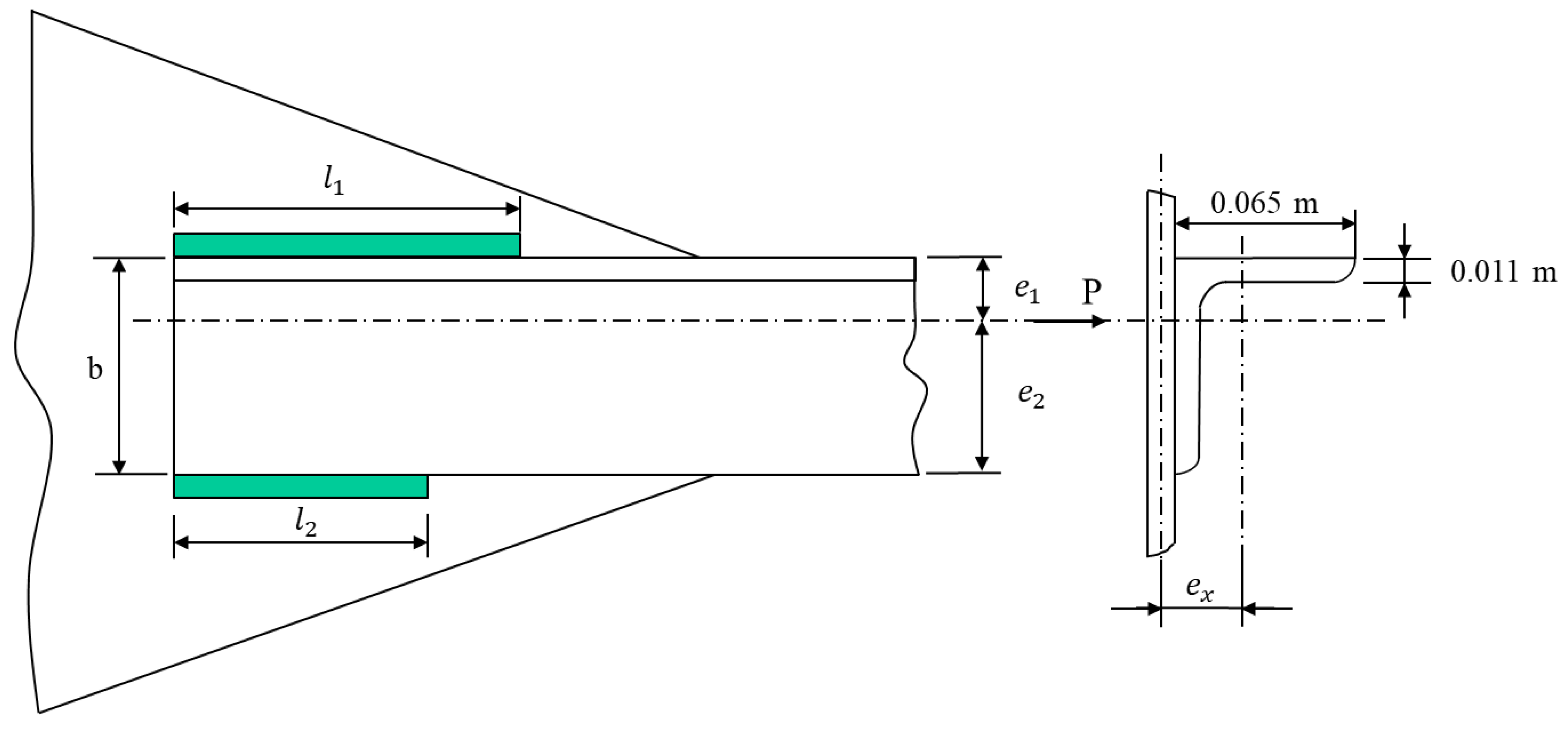
4.2. Case Study 2: Welded Gusset Optimal Design

A welded Gusset with the geometry as shown in Figure 10, was considered in this problem [32]. A profile $L$ $100\times 65\times 11 \left[\mathrm{mm}\right]$ with a section of $A=1.7\times {10}^{-3} {\mathrm{m}}^2$ must be welded to a $1.4\times {10}^{-3} \mathrm{m}$ thick plate so that the section of the profile can be subjected to tension in its totality. Considering that the base material is St37 steel (DIN 17100) with ${\sigma }_{\mathrm{adm}}\le 137.34 \mathrm{MPa}$ and the metal deposited in the fillet welds has ${\sigma }_{\mathrm{adm}, \mathrm{weld}}\le 107.91 \mathrm{MPa}$.

The welding cost includes the cost of preparing the joint to be welded, the cost of the material deposited, and the cost associated with the welding technology. Supposing that the cost can be expressed as a function of the welded joint dimensions, the following objective function is obtained:

$$\mathrm{Cos}\mathrm{t}=K\left(l_1\cdot a_1+l_2\cdot a_2\right),$$

(54)

where $K$ is associated with the price of the manpower and material costs, $l_1 \mathrm{and} l_2$ are the lengths of the fillet welds, and $a_1$ and $a_2$ are the respective widths of the projected weld throats according to the rules of the welding code design. In Figure 10, let’s consider the following data: $b=0.1 \mathrm{m}$, $e_1=0.034 \mathrm{m}$, and $e_x=0.0237 \mathrm{m}$.

To evaluate the normal stress caused by the bending moment, it is necessary to calculate the flexural strength module, $Z_f$:

$$Z_f=Z_{f1}+Z_{f2}$$

(55)

$$Z_{f1}={\displaystyle \frac{1}{6}}{l}_1^2{a}_1$$

(56)

$$Z_{f2}={\displaystyle \frac{1}{6}}{l}_2^2{a}_2$$

(57)

The normal stresses caused by the bending moment are defined as follows:

$$n={\displaystyle \frac{M_{\max }}{Z_f}},$$

(58)

where $M_{\max }=P\times e_x=5533.428 \mathrm{Nm}$.

The stress in the fillet welds (parallel to its longitudinal axis) is given as follows:

$$t_{//}={\displaystyle \frac{P}{l_1{a}_1+l_2{a}_2}},$$

(59)

where $P=A\times {\sigma }_{\mathrm{adm}}=233.47 \mathrm{kN}$.

Finally, according to the Portuguese regulation code on steel structures for buildings (REAE) [35], the equivalent stress ${\sigma }_{\mathrm{eq}}$, is given by the following:

$${\sigma }_{\mathrm{eq}}=\sqrt{1.4n^2+1.8t_{//}^2}$$

(60)

The stress constraint of the welded Gusset design problem is given by the following:

$${\sigma }_{eq}\le \overline{\alpha }{\sigma }_{adm,weld},$$

(61)

where $\overline{\alpha }$ is a safety factor, according to REAE (artº77) [35], successively defined as follows:

$${\alpha }_i=0.8\left(1+{\displaystyle \frac{1}{a_i}}\right), i=1, 2,$$

(62)

with the following:

$$a_i\ge 3 \left[\mathrm{mm}\right], i=1, 2$$

(63)

$$\overline{\alpha }=\min \left({\alpha }_i, i=1, 2\right)$$

(64)

The fitness function for this example is going to be calculated using the formulation from Equation (49) but using $C={10}^4, \lambda ={10}^{16} \mathrm{and} n=2$ so that no obtained solutions violate the constraints. The optimal reference point, obtained from [34], is the following:

$${\mathit{x}}^{*}=\left(5.13333, 5.13333, 400.0, 248.196\right)$$

(65)

$$f\left({\mathit{x}}^{*}\right)=3228.13$$

(66)

Results for the Case Study 2

The second example used the same stopping criteria as the first example. In terms of the best solutions obtained, presented in

Table 2. Best solutions obtained for Case Study 2.

Migration	Blending	Mutation	Crossover	Strategy	Local Search	${\mathit{x}}_1$	${\mathit{x}}_2$	${\mathit{x}}_3$	${\mathit{x}}_4$	Objective
Linear	No	Standard	$-$	$-$	No	5.152	5.446	383.299	240.904	3286.891
Linear	No	Taxonomic	$-$	$-$	No	5.433	5.833	385.931	220.302	3382.000
Linear	Yes	Standard	$-$	$-$	No	5.333	5.285	377.282	240.724	3284.266
Sinusoidal	Yes	Taxonomic	$-$	$-$	No	5.272	5.256	383.589	242.931	3299.102
Linear	No	Standard	$-$	$-$	Yes	5.162	4.751	400.000	250.000	3252.320
Linear	No	Taxonomic	$-$	$-$	Yes	5.370	4.460	400.000	248.257	3255.336
Linear	Yes	Standard	$-$	$-$	Yes	4.957	4.935	399.908	249.939	3215.531
Quadratic	Yes	Taxonomic	$-$	$-$	Yes	5.144	5.144	385.182	246.330	3248.703
Quadratic	Yes	Standard	SP	PEbS	No	5.265	5.262	382.206	238.214	3266.031
Quadratic	Yes	Standard	U	ISbF	No	5.243	5.241	382.236	240.257	3263.141
Linear	Yes	Standard	U	PEbS	Yes	4.945	4.945	400.000	250.000	3214.375
Linear	Yes	Standard	MP	ISbF	Yes	4.945	4.945	400.000	250.000	3214.375

, it is possible to note, once again, that the best solutions are improved when compared to the reference value. In this case, the use of the fully hybridized algorithm proved to be superior to the other approaches, as it repeatedly achieved the best solutions, even when using different crossover operators. This study is also a particularly good example of the benefits of adding crossover operators since, in both cases, with and without local search, their implementation helped to improve the final solution. The local search, once again, also proved its value by significantly improving the solution. On the downside, when the blending in migration was not used, the solution fell short of all the other cases, even with the help of the local optimizer. This is more than likely due to the non-blended migration since it does not introduce any diversity to the population by only replacing the bad solutions with the better ones. This feature, when combined with a complex function, can lead to a case like this one, where the algorithm was led to a local optimum and was never able to create a new solution outside of that point, which led to it being stuck at that point for several generations. This aspect is one of the biggest weaknesses of standard BBO algorithms, which has already been documented by other authors and is referred to as a lack of speed. Dan Simon [5] himself mentioned this lack of speed in his original paper. Hopefully, the concept of blending will solve this problem, even if only partially.

By using the evolution of the elite’s average fitness, Figure 11 once again shows the rapid decline in the first few generations of the algorithm. This figure, when compared with the previous figures, is also a good example of some of the problems that have occurred with the trapezoidal model, namely its inconsistency. This migration model was either one of the fastest or the slowest, the latter being more frequent. It also does not help that this model also shows poor synergy with the other modifications, specifically with taxonomic mutation. Figure 12 demonstrates a little bit of the influence of the crossover operator, with the curve of the graph being completely different from what is expected from this method. The conclusions are the following:

-

The fully hybridized model with the different options originally not included in the BBO continued to achieve the best results;

-

The inclusion of the crossover operator proved to be a good option, showing good results both with and without the use of the Hooke–Jeeves local optimizer. Both strategies achieved good results;

-

The Hooke–Jeeves local optimizer continued to be an advantage, showing several robust results;

-

The migration model with blending was an asset. In this example, we can see its impact on synergy with the other hybridization options, especially the Hooke–Jeeves local optimizer;

-

The linear migration model was the most prevalent in this case;

-

Both mutations achieved good results, but the taxonomic mutation showed worse synergy when integrated with other options, slowing down the algorithm in some cases.

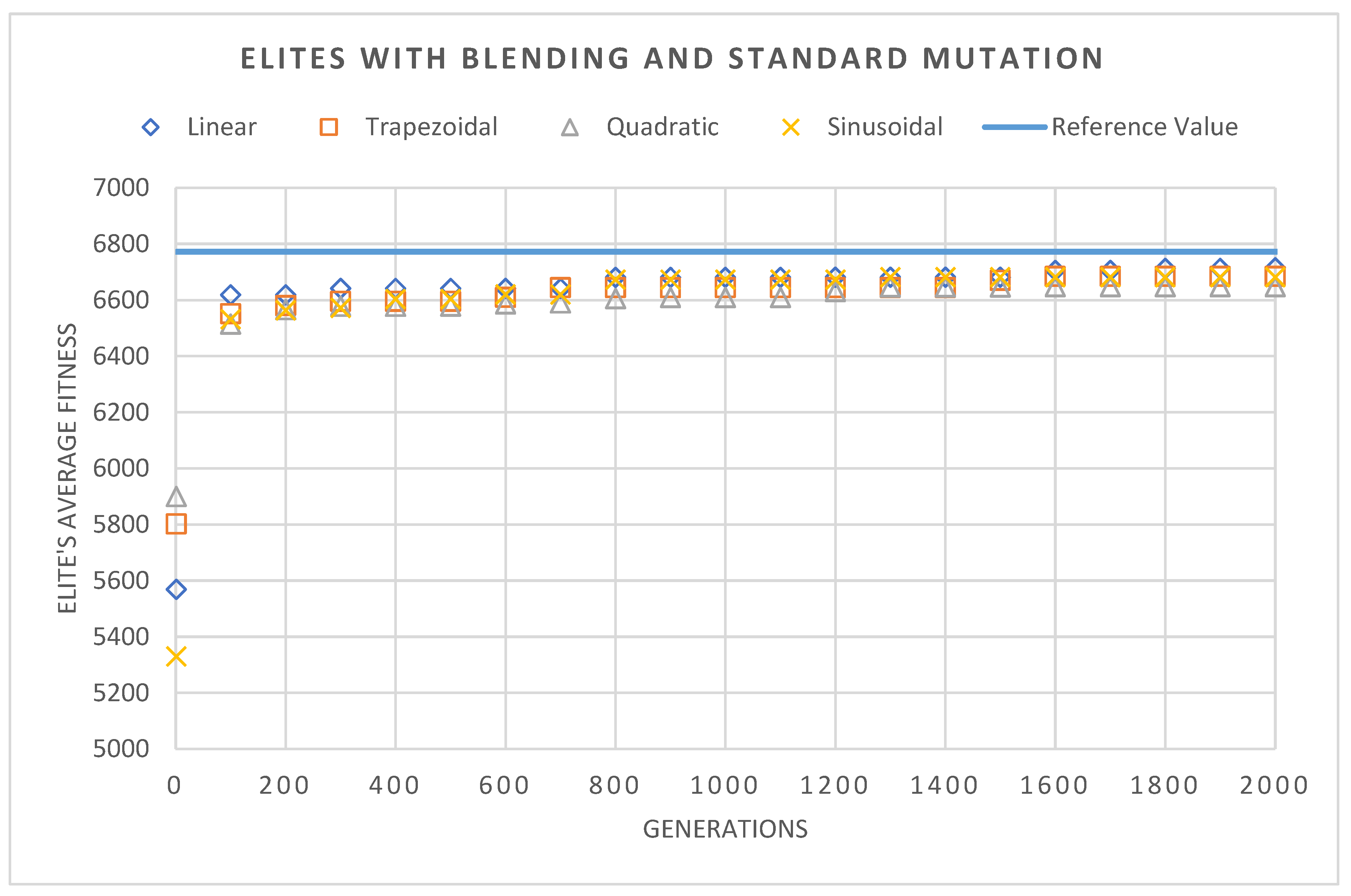
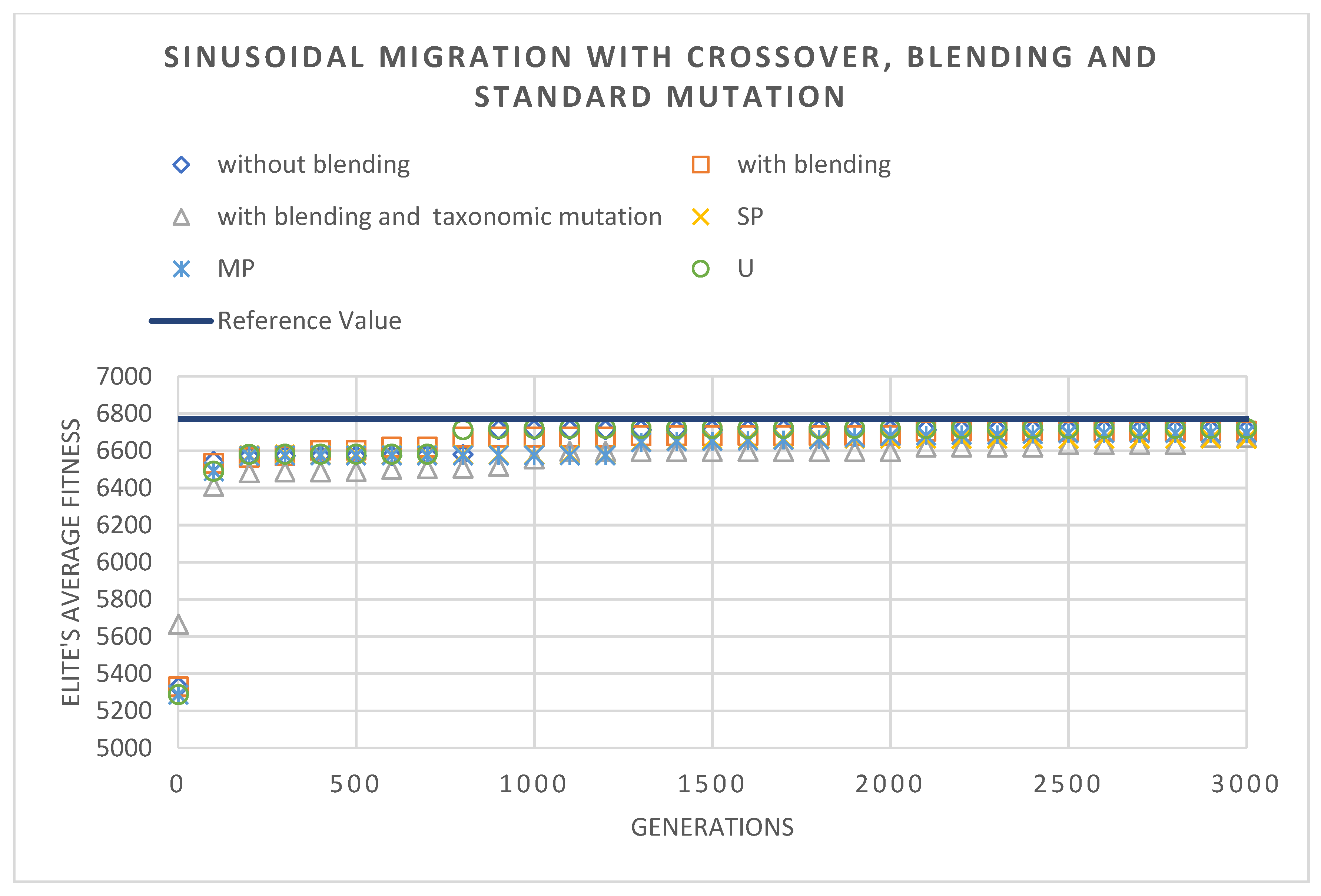
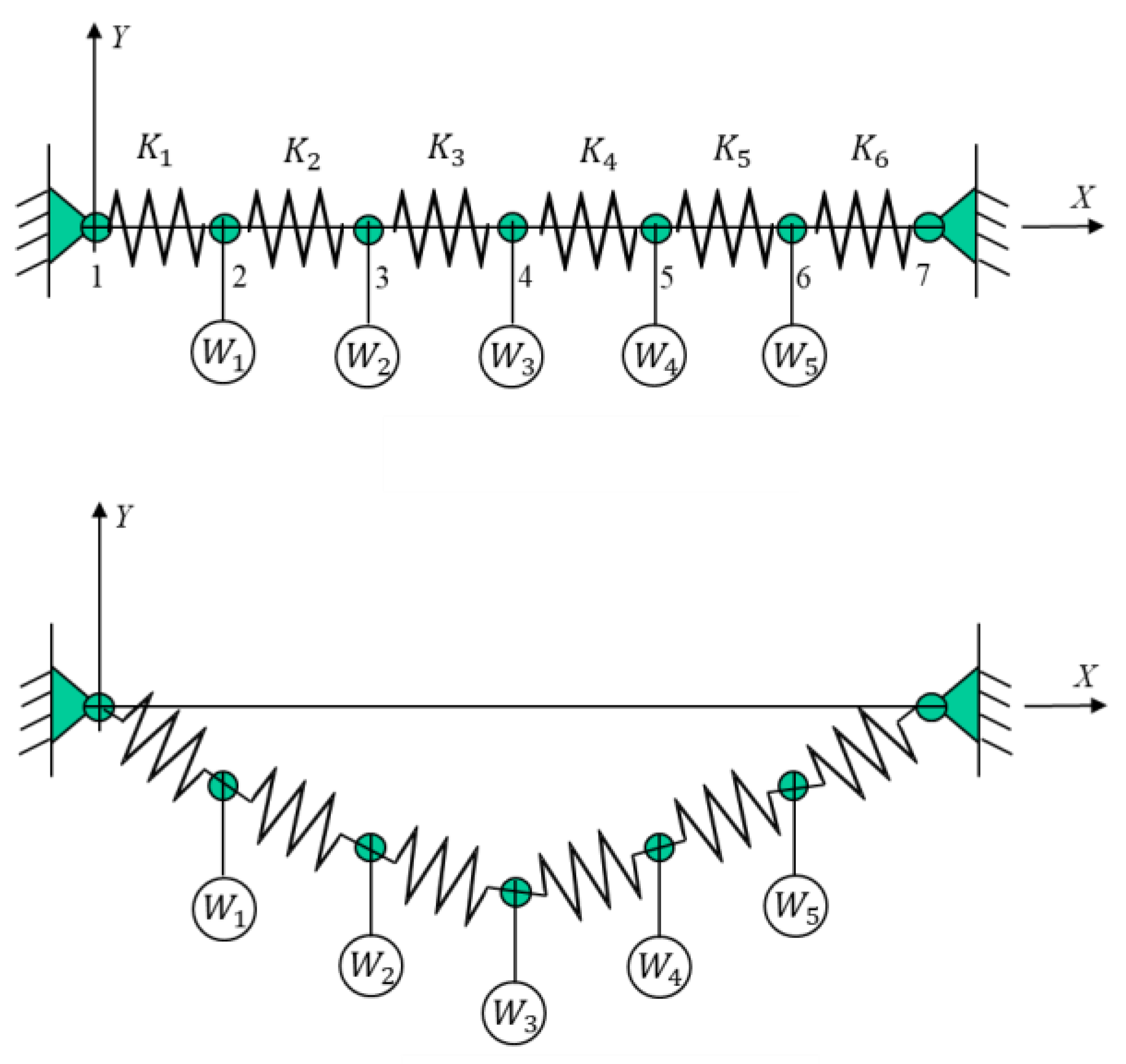
4.3. Case Study 3: Design of Springs and Weights System

Figure 13 shows a spring system supporting weights at the connections between the springs [36]. First, the system analysis was performed to determine the equilibrium position by minimizing the potential energy. For this, five weights and six springs were considered.

The $i$-th spring deformation is given by the following equation:

$$\mathsf{\Delta }{L}_i={\left[{\left(x_{i+1}-x_i\right)}^2+{\left(y_{i+1}-y_i\right)}^2\right]}^{{\displaystyle \frac{1}{2}}}-L_i^0,$$

(67)

with $L_i^0=10 \mathrm{m}$.

There are $N+1$ springs, with $N$ being the number of weights ($N=5$ in this case). The stiffness of the $i$-th spring is the following:

$$K_i=500+200{\left({\displaystyle \frac{N}{3}}-i\right)}^2 \left[\mathrm{N}/\mathrm{m}\right],$$

(68)

and the weight applied at the $j$-th node is given as follows:

$$W_j=50j \left[\mathrm{kg}\right]$$

(69)

The potential energy of the system is then given by the following:

$$PE=\sum _{i=1}^{N+1}{\displaystyle \frac{1}{2}}{K}_i{\left(\Delta L_i\right)}^2+\sum _{j=1}^K{W}_j\cdot y_{j+1}$$

(70)

The design variables are the nodes’ position in the spring-deformed state. Therefore, the design variables are $x_i, i=2,\dots , 6$ and $y_i, i=2,\dots , 6$, for a total of ten design variables. The fitness function used is going to be Equation (70), and the only constraints applied to the problem will be the size constraints so that the solution obtained ensures that no nodes interfere with each other in a physically impossible manner. The optimal solution described in the book [36] is given as follows:

$$PE\left({\mathit{x}}^{\mathit{*}}\right)=-4416 J$$

(71)

Results for the Case Study 3

After analyzing the best solutions obtained, as shown in

Table 3. Best solutions obtained for Case Study 3(The bold is to highlight the solutions that were better than the reference value).

Migration	Blending	Mutation	Crossover	Strategy	Local Search	${\mathit{x}}_1$	${\mathit{x}}_2$	${\mathit{x}}_3$	${\mathit{x}}_4$	${\mathit{x}}_5$	${\mathit{x}}_6$	${\mathit{x}}_7$	${\mathit{x}}_8$	${\mathit{x}}_9$	${\mathit{x}}_{10}$	Objective
Linear	No	Standard	$-$	$-$	No	10.661	21.662	32.472	42.576	52.798	−1.074	−6.640	−8.149	−8.245	−6.338	−2672.011
Linear	No	Taxonomic	$-$	$-$	No	9.693	20.007	32.468	41.354	50.033	−5.157	−5.452	−8.277	−4.353	−1.409	1365.146
Linear	Yes	Standard	$-$	$-$	No	10.687	21.898	32.099	42.324	51.633	−4.513	−8.426	−11.010	−9.361	−5.726	−4092.193
Quadratic	Yes	Taxonomic	$-$	$-$	No	9.623	21.124	31.305	41.743	51.953	−6.019	−9.242	−10.971	−9.279	−6.374	−3823.344
Linear	No	Standard	$-$	$-$	Yes	10.661	21.662	32.472	42.576	52.798	−1.074	−6.640	−8.149	−8.245	−6.338	−2672.01
Trapezoidal	Yes	Standard	$-$	$-$	Yes	10.331	21.037	31.642	42.043	51.727	−4.289	−7.907	−9.817	−9.330	−5.954	−4415.8
Trapezoidal	Yes	Taxonomic	$-$	$-$	Yes	10.260	20.769	31.299	41.583	51.383	−4.159	−7.885	−9.418	−8.652	−5.501	−4354.79
Linear	Yes	Standard	U	PEbS	No	10.260	20.769	31.299	41.583	51.383	−4.159	−7.885	−9.418	−8.652	−5.501	−4354.79
Linear	Yes	Standard	MP	ISbF	No	10.138	21.365	31.552	41.634	51.231	−4.565	−6.713	−8.980	−8.843	−5.249	−4151.46
Quadratic	Yes	Standard	SP	PEbS	Yes	10.347	21.076	31.679	42.082	51.764	−4.292	−7.914	−9.860	−9.390	−6.003	−4416.36
Sinusoidal	Yes	Standard	U	ISbF	Yes	10.349	21.078	31.679	42.080	51.766	−4.286	−7.892	−9.840	−9.377	−6.005	−4416.36

, it is important to note that only the fully hybridized method was able to reach the reference solution. The worst solution came, once again, from the tests without blending and with taxonomic mutation, assuming that the same reasons that plagued the two previous problems also hold true here. The addition of the crossover operators was, once again, very beneficial; their addition allowed for an improvement of solutions. Furthermore, both strategies performed well and were able to provide valuable solutions equally. The linear model of migration also seems to continue its dominance, having a lot of placements, but this time, the best solutions came from different models.

In terms of the evolution of the elite’s average fitness with the generations, Figure 14 shows more of the same behavior. The steep initial drop and the intermediate and final slump, which remain in a non-optimal solution. Figure 15 on the other hand showed a behavior similar to other GAs, this mainly shows the influence that the crossover operators had in this example, demonstrating, once again, its benefits.

However, this example highlighted a problem that affected the algorithm’s performance, slowing it down. This error arose with the use of taxonomic mutation together with crossover operators. In fact, in the initial generations, due to the generation of bad solutions in the recombination process, the performance of the differential taxonomic mutation worsened significantly. Using these bad solutions from the crossover worsens the quality of the population, thus reducing the convergence rate. However, this problem can be easily solved by using a solution selection process after the generation of offspring during the crossover, preventing very bad solutions from entering the new population, or by adopting a hybrid mutation strategy based on the BBO method’s standard mutation in the initial generations and taxonomic mutation in the intermediate and final generations. The conclusions are the following:

-

The algorithm presented more difficulties in this example but managed to obtain solutions close to the reference value when fully hybridized;

-

Both options included (crossover and local optimizer) had an impact, with the local optimizer being the most important;

-

The linear model continued to have the best performance, but the other non-linear models obtained the best results in the end;

-

Standard mutation obtained the best results due to a problem that differential mutation had with the bad solutions coming from the crossover operators;

-

Migration with blending has continued to be an impactful modification, and this example demonstrates it well.

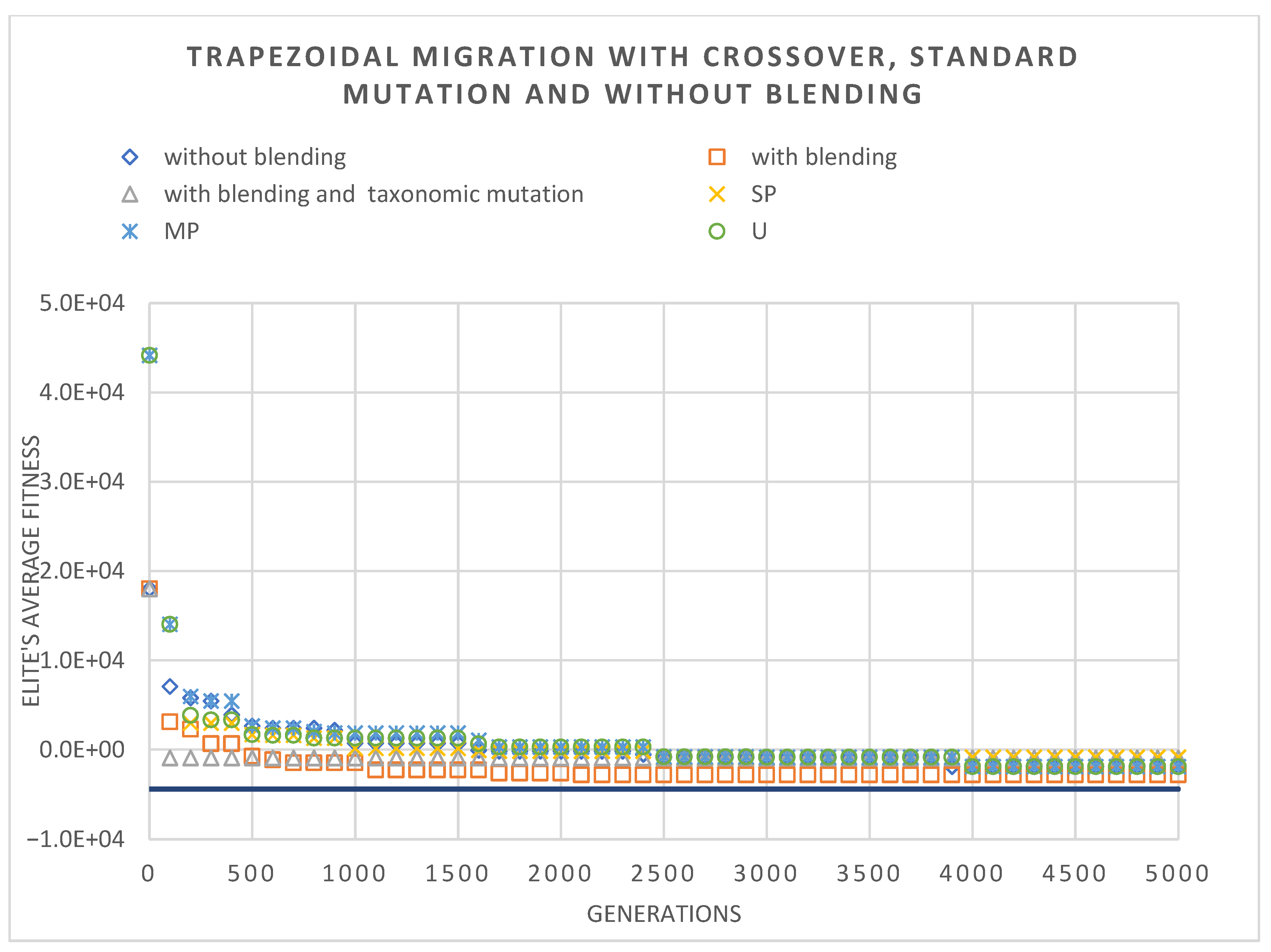
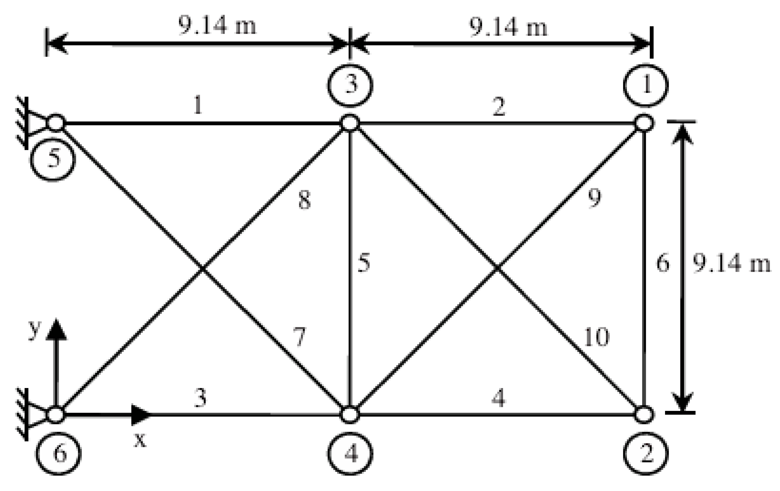
4.4. Case Study 4: The 10-Bar Truss

The objective of this problem is to minimize the mass of the structure by varying the cross-sectional area of the elements while respecting the limitations and restrictions based on stresses and displacements. Figure 16 shows the geometry that is going to be studied in this example from [37].

The structure is loaded on nodes 2 and 4 by two vertical loads (one per node) of $P_y=-4.45\times {10}^5 \mathrm{N}$. The Young’s modulus of the material is $E=6.9\times {10}^8 \mathrm{N}/{\mathrm{m}}^2$.

The objective function of the problem is the following:

$$f\left(x\right)=\rho {\sum }_{i=1}^{10}{A}_i{l}_i,$$

(72)

where $\rho =2.77\times {10}^3 \mathrm{kg}/{\mathrm{m}}^3$ represents the density, $l_i$ the length of the element, and $A_i$ the cross-section area of the element.

The constraint values for the stresses and displacements are $\left|\sigma \right|\le 1.72\times {10}^8 \mathrm{N}/{\mathrm{m}}^2$ (traction/compression) and $\left|\delta \right|\le 5.08\times {10}^{-2} \mathrm{m}$, respectively. The cross-sectional areas of members must belong to the interval from $6.45\times {10}^{-5} {\mathrm{m}}^2$ to $2.26\times {10}^{-2} {\mathrm{m}}^2$.

The reference value from [37], which was obtained using an AGA (augmented genetic algorithm), is presented below:

$$f\left({\mathit{x}}^{*}\right)=2261.42 \left[\mathrm{kg}\right]$$

(73)

It is also important to note that the linear equation system was solved using Gaussian elimination with partial pivoting.

Results for the Case Study 4

The best solutions presented in

Table 4. Results for Case Study 4, the 10-bar truss example.

Migration	Blending	Mutation	Crossover	Strategy	Local Search	${\mathit{x}}_1$	${\mathit{x}}_2$	${\mathit{x}}_3$	${\mathit{x}}_4$	${\mathit{x}}_5$	${\mathit{x}}_6$	${\mathit{x}}_7$	${\mathit{x}}_8$	${\mathit{x}}_9$	${\mathit{x}}_{10}$	Objective
Trapezoidal	No	Standard		$-$	No	0.0156	0.0166	0.0224	0.0183	0.000108	0.00548	0.0135	0.02	0.00635	0.0225	4221.072
Linear	No	Taxonomic		$-$	No	0.0226	0.0226	0.0226	0.0129	0.000315	0.0226	0.0226	0.0226	0.00374	0.0226	5189.495
Trapezoidal	Yes	Standard		$-$	No	0.0205	0.000506	0.0212	0.0141	0.000407	0.0106	0.00353	0.0204	0.0173	0.0214	3946.545
Linear	Yes	Taxonomic		$-$	No	0.0215	0.0154	0.0177	0.0224	0.00825	0.00695	0.0225	0.0209	0.00915	0.021	4974.689
Quadratic	No	Standard		$-$	Yes	0.00536	0.000065	0.0226	0.0226	0.0000645	0.0000645	0.00531	0.0199	0.0000645	0.0226	3002.792
Linear	No	Taxonomic		$-$	Yes	0.0205	0.0226	0.0223	0.013	0.0000645	0.0073	0.0225	0.00992	0.0203	0.0226	4873.072
Trapezoidal	Yes	Standard		$-$	Yes	0.000397	0.000065	0.0195	0.0114	0.0000645	0.000398	0.00353	0.0158	0.000567	0.0197	2226.827
Sinusoidal	Yes	Taxonomic		$-$	Yes	0.00098	0.000065	0.0179	0.0213	0.0000645	0.00476	0.00437	0.0226	0.0000645	0.0222	2908.027
Linear	Yes	Taxonomic	MP	PEbS	No	0.000213	0.000065	0.0197	0.00961	0.0000645	0.00032	0.00352	0.0188	0.00185	0.0171	2234.67
Linear	Yes	Taxonomic	SP	ISbF	No	0.000065	0.000065	0.0158	0.0132	0.0000645	0.000509	0.00366	0.0203	0.00186	0.0168	2280.885
Sinusoidal	Yes	Standard	U	PEbS	Yes	0.000725	0.000066	0.0226	0.0108	0.0000651	0.000925	0.00346	0.0166	0.00152	0.0144	2182.267
Quadratic	Yes	Standard	MP	ISbF	Yes	0.000684	0.000065	0.0215	0.0141	0.0000677	0.00101	0.00348	0.0146	0.00138	0.0152	2190.475

show that in the majority of the tests, the algorithm did not reach a value close to the reference value; this may be due to the combination of the complexity of the problem and the limitation created by the stopping criteria, which, once again, was placed as 5000 generations. However, on a positive note, there were also many results that were better than the reference value. In terms of migration models, it is important to note the good synergy that the linear model continues to show, having great results with all of the modifications. The sinusoidal model, which obtained the best value, and the trapezoidal model, which consistently obtained the best values for the respective test, should also be highlighted. This example also proved that with a more complex migration model, it is possible to obtain better results. On the side of the mutation operator, both operators (standard and taxonomic) were able to reach good values, but it is important to highlight that when the local search was used, the standard mutation was better. This factor, combined with the fact that linear migration is the model that behaves best with taxonomic mutation, shows some of the synergy problems that have already been exposed here. Finally, the crossover operator also proved to be a positive influence in this case, allowing for the improvement of the solutions.

By analyzing the evolution of the elite’s average fitness, presented in Figure 17 and Figure 18, it is possible to witness the same phenomenon mentioned before. By highlighting the first graph, it is possible to see the influence of the local search, with the steady increase in value on the trapezoidal model curve. In addition, this graph shows the dominance of the sinusoidal model, which, without that huge spike in the value of the trapezoidal model, would be the best in these tests. The second graph also shows some interesting behaviors, especially the uniform crossover (U), which shows a very steady increase in the value of the elite’s average fitness over the generations. The curves relating to the use of the crossover operator show better algorithmic performance.

-

The inclusion options (crossover and local optimizer) had quite an impact. The fully hybridized algorithm obtained the best results;

-

This example has shown that for more complex problems, more complex migration models obtain better results. However, the linear model manages to overcome this advantage in some cases with its good synergy with other techniques;

-

The model, without hybridization, struggled to achieve reasonable results;

-

The migration model with blending maintained its good performance, especially during tests including other hybridization options;

-

The model with standard mutation obtained the best results, but taxonomic mutation also performed well.

5. Statistical Tests

To better understand the impact of the new additions to the method, the best results obtained were subjected to data analysis using statistical tests, namely the Friedman [38] and Wilcoxon [39] tests. The migration statistical tests studied the significance of the differences between the different migration models (linear, trapezoidal, quadratic, and sinusoidal), and the mutation tests studied the significance of the differences between the two migration operators (standard mutation and taxonomic mutation). The tests relating to the crossover operator studied the significance of using the crossover operator, and tests were also carried out to study the different crossover operators (Single-Point, Mult-Point, and Uniform) subject to two different Matrix Selection Mechanisms (PEbs and ISbF). Finally, the significance of the differences between having local search active or not active was also studied. The results of these tests are shown in

Table 5. Results for the statistical tests according to Friedman [38] and Wilcoxon [39] tests(The bold is to highlight the values that are lower than the normal significance value of 0.05).

Case Study	Test	Test Statistic	p-Value
1	Migration	0.9344	0.8171
	Mutation	3	0.4652
	Crossover	4	0.3452
	Crossover Operators (PEbS)	8.4	0.01499
	Crossover Operators (ISbF)	6	0.04978
	Local Search	0	0.02771
2	Migration	2.636	0.4512
	Mutation	0	0.03125
	Crossover	5	0.5002
	Crossover Operators (PEbS)	0.6667	0.7165
	Crossover Operators (ISbF)	0.1333	0.9355
	Local Search	0	0.02771
3	Migration	0.5556	0.9065
	Mutation	0	0.125
	Crossover	0	0.1797
	Crossover Operators (PEbS)	2	0.3679
	Crossover Operators (ISbF)	4.667	0.09697
	Local Search	0	0.1088
4	Migration	0.5056	0.9177
	Mutation	5	0.3125
	Crossover	0	0.125
	Crossover Operators (PEbS)	1.5	0.4724
	Crossover Operators (ISbF)	0.5	0.7788
	Local Search	1	0.0625

for all cases.

From Table 5, the following conclusions can be established:

• As observed, there are only five values below the normal significance value (α = 0.05), which means that these tests (marked in bold) were the only ones in which the difference between parameters was significant enough to reject the null hypothesis;
• It can also be seen that local research, on average, has the lowest p-value, so it can be concluded that its introduction has had the greatest impact on the method;
• It is also important to note that the differences between the different migration models were not as significant as the other additions since, on average, the p-value is the highest of all the tests;
• The values obtained in the mutation tests are also very interesting, with the second lowest average p-value, which may be due to the problems that were described in Case Study 3, with the use of the crossover and taxonomic mutation operators, a problem that also arose in Case Study 2, the two case studies with the lowest p-value for mutation.

6. Conclusions

An evolutionary algorithm based on biogeography (BBO) was implemented to be applied to various problems in the topic of optimization of mechanical systems and to study their behavior. This work adapted not only the linear migration model from Dan Simon’s original work [5] but also the trapezoidal, quadratic, and sinusoidal models presented in Ma’s work [7]. In terms of mutation operators, the standard BBO mutation and Hao’s taxonomic mutation were implemented [28]. The initial algorithm was later hybridized with other concepts and heuristics from other methods, such as the crossover operators Single-Point (SP), Multiple-Point (MP), and Uniform (U) used in genetic algorithms and local search-based learning from the memetic algorithm’s idea.

The standard non-hybridized BBO showed its best performance in the initial generations due to its good global search. However, the results obtained fell short of the benchmarks in the literature using other optimization methods. This poor performance was due to the lack of diversity of solutions in the populations at the final generations of the optimization process. This feature is associated with the replacement of solutions of the migration operator, an intrinsic property of the BBO method. The addition of the blending strategy, applied during the migration process and introduced by Dan Simon, the original author of BBO, proved to be very beneficial, improving the algorithm’s performance in several respects. Even so, some of BBO’s initial problems persisted. Thus, other processes, such as the injection of new solutions [24,25] before BBO hybridization, have proved effective in improving population diversity. The results obtained after these inclusions proved to be positive.

In terms of migration, the models that stood out the most during the tests were the sinusoidal and linear models, which managed to produce several optimal results. The quadratic model, although less consistent, also managed to produce satisfactory results, outperforming the other models in some cases. The worst model, the trapezoidal model, showed reliable results but was the slowest and most inconsistent when compared to the other models. In addition, this model also showed poor synergy with the other operators implemented, such as taxonomic mutation and the local optimizer. The standard mutation and taxonomic mutation operators were able to produce good results when migration with blending was used. Standard mutation prioritized the speed of the algorithm, generating good solutions quickly, while taxonomic mutation showed greater precision at the cost of some speed.

The hybridization process began with the implementation of the crossover operators, which required the implementation of binary coding of solutions. The three implemented crossover operators were subject to two different mating selection strategies. The inclusion of these operators proved to be positive, with an improvement in results in general. The second mating selection strategy (ISbF) appeared to have better behavior, especially when used in conjunction with the MP (Multiple-Point) crossover operator, but the first mating selection strategy (PEbS) was also quite positive. The three crossover operators obtained satisfactory, fairly similar results and showed good synergy with the other operators and concepts, especially with blending migration.

Then, the Hooke–Jeeves local optimizer was implemented, which presented excellent results, even in the tests without the inclusion of the crossover. However, the best results were obtained when the fully hybridized algorithm was used. Thus, the algorithm was able not only to quickly reach the optimum points but also, in some cases, to surpass them.

When the algorithm was exposed to a more complex problem, it presented some difficulties, initially without the use of hybridization. However, with the inclusion of crossover operators and local search, it managed to achieve good values, albeit with some struggle. This example also showed that complex migration models have an easier time dealing with complex problems. However, it also showed that the greatest advantage of the linear migration model, its great synergy with the other modifications, allowed it to compete with the more complex models.

In conclusion, the initial behavior of the BBO original method suggested that it needed some improvements to reach its true potential. With the proposal innovations, the method showed excellent results, achieving its objective with relative ease. It can be said that these innovations complement the method positively and that their inclusion should be further strengthened.

With this being said, there are still some issues present in the hybridized method. Initially, the computation for the $A^{\prime }$ matrix still brings some issues in terms of speed, and, most importantly, it also can affect the size of the population, which is a big problem, especially considering that this method has a big problem in terms of population diversity. It could also be interesting to further the hybridization and continue to implement other heuristics and operators from other optimization methods, specifically concepts related to local search and local optimization, such as Svanberg’s method of moving asymptotes. Other modifications could also be implemented, this time focusing on the processes added through hybridization, like changing the Hooke–Jeeves method so that it searches a larger local area. There is also a possibility of using crossover operators in the real domain to create a better synergy between the crossover operators and the BBO operators.

References

1. Holland, J. Genetic Algorithms. Sci. Am. 1992, 267, 66–73. [Google Scholar] [CrossRef]
2. Dawkins, R. The Selfish Gene; Oxford University Press: Oxford, UK, 1976. [Google Scholar]
3. Lamarck, J.B. Zoological Philosophy; Macmillan and Co.: London, UK, 1914. [Google Scholar]
4. Mark Baldwin, J. A New Facctor in Evolution. Am. Natl. 1869, 30, 354. [Google Scholar]
5. Simon, D. Biogeography-based optimization. IEEE Trans. Evol. Comput. 2008, 12, 702–713. [Google Scholar] [CrossRef]
6. Ma, H.; Simon, D.; Siarry, P.; Zhile, Y.; Fei, M. Biogeography-Based Optimization: A 10-Year Review. IEEE Trans. Emerg. Top. Comput. Intell. 2017, 1, 391–406. [Google Scholar] [CrossRef]
7. Ma, H. An analysis of the equilibrium of migration models for biogeography. Inf. Sci. 2010, 180, 3444–3464. [Google Scholar] [CrossRef]
8. Ma, H.; Simon, D. Blended biogeography-based optimization for constrained optimization. Eng. Appl. Artif. Intell. 2011, 24, 517–525. [Google Scholar] [CrossRef]
9. Boussaïd, I.; Chatterjee, A.; Siarry, P.-N.M. Biogeography-based optimization for constrained optimization problems. Comput. Oper. Res. 2012, 39, 3293–3304. [Google Scholar] [CrossRef]
10. Bi, X.; Wang, J. Constrained Optimization Based on Epsilon Constrained Biogeography-Based Optimization. Int. Conf. Intell. Hum.-Mach. Syst. Cybern. 2012, 2, 369–372. [Google Scholar]
11. Ma, H.; Ruan, X.; Pan, Z. Handling multiple objectives with biogography-based optimization. Int. J. Autom. Comput. 2012, 9, 30–36. [Google Scholar] [CrossRef]
12. Bi, X.; Wang, J.; Li, B. Multi-objective optimization based in hybrid biogeography-based optimization. Syst. Eng. Electron. 2014, 36, 179–186. [Google Scholar]
13. Xu, Z. Study on Multi-Objective Optimization Theory and Application Based on Biogeography Algorithm. Ph.D. Thesis, Harbin Engineering University, Harbin, China, 2013. [Google Scholar]
14. Kundra, H.; Sood, M. Cross-Country Path Finding using Hybrid approach of PSO and BBO. Internatuinal J. Comput. Appl. 2010, 7, 15–19. [Google Scholar] [CrossRef]
15. Albrase, F.; Alroomi, A.; Talaq, J. Optimal Coordination of Directional Overcurrent Relays Using Biogeography-Based Optimization Algorithm. IEEE Trans. Power Deliv. 2015, 30, 1810–1820. [Google Scholar]
16. Gong, W.; Cai, Z.; Ling, C. “DE/BBO: A hybrid differential evolution with biogeography.based optimization for global numerical optimization. Soft Comput. 2010, 15, 645–665. [Google Scholar] [CrossRef]
17. Boussaid, I.; Chatterjee, A.; Siarry, P.; Ahmed-Nacer, M. Hybridizing Biogeography-Based Optimization With Differential Evolution for Optimal Power Allocation in Wireless Sensor Networks. IEEE Trans. Veh. Technol. 2011, 60, 2347–2353. [Google Scholar] [CrossRef]
18. Bhattacharya, A.; Chattopadhyay, P.K. Hybrid differential evolution with biogeography-based optimization algorithm for solution of economic emission load dispatch problems. Expert Syst. Appl. 2011, 38, 14001–14010. [Google Scholar] [CrossRef]
19. Panchal, V.; Jundra, H.; Kaur, A. An Integrated Approach to Biogeography Based Optimization with case based reasoning for retrieving Groundwater Possibility. J. Technol. Eng. Sci. 2010, 1, 32–38. [Google Scholar]
20. Wang, L.; Xu, Y. An effective hybrid biogeography-based optimization algorithm for parameter estimation of chaotic systems. Expert Syst. Appl. 2011, 38, 15103–15109. [Google Scholar] [CrossRef]
21. Arora, P.; Jundra, H.; Panchal, V. Fusion of Biogeography based optimization and Artificial bee colony for identification of Natural Terrain Features. Int. J. Adv. Comput. Sci. Appl. 2012, 3. [Google Scholar] [CrossRef]
22. Wang, G.-G.; Guo, L.; Duan, H.; Shao, M. Hybridizing Harmony Search with Biogeography Based Optimization for Global Numerical Optimization. J. Comput. Theor. Nanosci. 2013, 10, 2312–2322. [Google Scholar] [CrossRef]
23. Zhao, B.; Deng, C.; Yang, Y.; Peng, H. Novel Binary Biogeography-Based Optimization Algorithm for the Knapsack Problem. In Proceedings of the International Conference in Swarm Intelligence, Shenzhen, China, 17–20 June 2012. [Google Scholar]
24. Conceição António, C.A. A hierarchical genetic algorithm for reliability based design of geometrically non-linear composite structures. Compos. Struct. 2001, 54, 37–47. [Google Scholar] [CrossRef]
25. Conceição António, C.A. A multilevel genetic algorithm for optimization of geometrically nonlinear stiffened composite structures. Struc. Multidisc. Optim. 2002, 24, 372–386. [Google Scholar] [CrossRef]
26. Wilson, E.O.; MacArthur, R. The Theory of Island Biogeography; Princeton University Press: Princeton, NJ, USA, 1967. [Google Scholar]
27. Zheng, Y.; Sueqin, L.; Zhang, M.; Chen, S. Biogeography-Based Optimization: Algorithms and Applications; Science Press Beijing: Beijing, China, 2019. [Google Scholar]
28. Hao, J.; Zhao, X.; Ji, Y. A Novel Biogeography-Based Optimization Algorithm with Momentum Migration and Taxonomic Mutation. Adv. Swarm Intell. 2020, 12145, 83–93. [Google Scholar]
29. António, C.C. Optimization of Mechanical Systems; Efeitos Gráficos: Porto, Portugal, 2022. [Google Scholar]
30. Eshelman, L.; Caruana, A.; Schaffer, J. Biases in the crossover landscape. In Proceedings of the Third International Conference on Genetic Algorithms, Fairfax, VA, USA, 4–7 June 1989; pp. 10–19. [Google Scholar]
31. Peixoto, A. Modelo de Otimização Biogeográfico Hibridizado com Algoritmos Meméticos para Conceção Ótima de Sistemas Mecânicos; Faculdade de Engenharia da Universidade do Porto: Porto, Portugal, 2024. [Google Scholar]
32. António, C.A.C.; Carneiro, G.M.P.N. Optimization of Mechanical Systems: Optimal Design Applications; Efeitos Gráficos: Porto, Portugal, 2022. [Google Scholar]
33. “Welded Beam Design Optimization”, MAPLE. Available online: https://www.maplesoft.com/support/help/maple/view.aspx?path=applications%2FWeldedBeam (accessed on 1 March 2024).
34. Gonçalves, H.F.S. Development and Implementation of Memetic Models for the Optimal Design of Mechanical Systems; Faculdade de Engenharia da Universidade do Porto: Porto, Portugal, 2023. [Google Scholar]
35. REAE. Decreto-Lei nº 21/86. In Regulamento de Estruturas de Aço para Edifícios; Imprensa Nacional Casa da Moeda: Lisbon, Portugal, 1986. [Google Scholar]
36. Vanderplaats, G.N. Numerical Optimization with MATLAB Programming; McGraw Hill: New York, NY, USA, 1984. [Google Scholar]
37. Aminifar, F.; Aminifar, F.; Nazarpour, D. Optimal design of truss structures via an augmented genetic algorithm. Turk. J. Eng. Environ. Sci. 2013, 37, 56–68. [Google Scholar]
38. Friedman, M. The use of ranks to avoid the assumption of normality implicit in the analysis of variance. J. Am. Stat. Assoc. 1937, 32, 674–701. [Google Scholar] [CrossRef]
39. Wilcoxon, F. Individual Comparisons by Ranking Methods. Biom. Bull. 1945, 1, 80–83. [Google Scholar] [CrossRef]
Figure 1. Flowchart of the standardized BBO method.
Mathematics 13 00492 g001
Figure 2. Graphical representation of the linear migration model [7].
Mathematics 13 00492 g002
Figure 3. Graphic representation of the trapezoidal migration model [7].
Mathematics 13 00492 g003
Figure 4. Graphic representation of the quadratic migration model [7].
Mathematics 13 00492 g004
Figure 5. Graphic representation of the sinusoidal migration model [7].
Mathematics 13 00492 g005
Figure 6. Flow diagram of the hybridized BBO [31].
Mathematics 13 00492 g006
Figure 7. Welded beam system.
Mathematics 13 00492 g007
Figure 8. Evolution of the elite’s average fitness through two thousand generations.
Mathematics 13 00492 g008
Figure 9. Evolution of the elite’s average fitness through two thousand generations, with local search (LS).
Mathematics 13 00492 g009
Figure 10. Welded Gusset design problem.
Mathematics 13 00492 g010
Figure 11. Evolution of the elite’s average fitness through two thousand generations.
Mathematics 13 00492 g011
Figure 12. Evolution of the elite’s average fitness through three thousand generations, with the crossover operator.
Mathematics 13 00492 g012
Figure 13. Schematic description of a spring and weight system.
Mathematics 13 00492 g013
Figure 14. Evolution of the elite’s average fitness through two thousand generations.
Mathematics 13 00492 g014
Figure 15. Evolution of the elite’s average fitness through five thousand generations, with the crossover operator, taxonomic mutation, and local search.
Mathematics 13 00492 g015
Figure 16. The 10-bar truss structure.
Mathematics 13 00492 g016
Figure 17. Evolution of the elite’s average fitness through five thousand generations.
Mathematics 13 00492 g017
Figure 18. Evolution of the elite’s average fitness through 5000 generations, with the crossover operators (SP-single point, MP-multipoint, U-uniform) with or without blending and taxonomic mutation.
Mathematics 13 00492 g018