A Dual Tandem Queue as a Model of a Pick-Up Point with Batch Receipt and Issue of Parcels

Abstract

Parcel delivery networks have grown rapidly during the last few years due to the intensive evolution of online marketplaces. We address the issue of managing the operation of a network’s pick-up point, including the selection of the warehouse’s capacity and the policy for accepting orders for delivery. The existence of the time lag between order placing and delivery to the pick-up point is accounted for via modeling the order’s processing as the service in the dual tandem queueing system. Distinguishing features of this tandem queue are the account of possible irregularity in order generation via consideration of the versatile Markov arrival process and the possibilities of batch transfer of the orders to the pick-up point, group withdrawal of orders there, and client no-show. To reduce the probability of an order rejection at the pick-up point due to the overflow of the warehouse, a threshold strategy of order admission at the first stage on a tandem is proposed. Under the fixed value of the threshold, tandem operation is described by the continuous-time multidimensional Markov chain with a block lower Hessenberg structure for the generator. Stationary performance measures of the tandem system are calculated. Numerical results highlight the dependence of these measures on the capacity of the warehouse and the admission threshold. The possibility of the use of the results for managerial goals is demonstrated. In particular, the results can be used for the optimal selection of the capacity of a warehouse and the policy of suspending order admission.

1. Introduction

Due to the influence of versatile economic, technological, social, etc., factors, including, in particular, the intensive evolution of online marketplaces and the COVID-19 pandemic, the order delivery industry has increased in size very rapidly during recent years. Parcel (order) delivery via the use of pick-up points is very popular as a solution for goods and food delivery on different online marketplaces, e.g., Amazon, eBay, Rakuten, Shopee, AliExpress, Etsy, Walmart, Mercado Libre, Wildberries, Ozon, Taobao, Tmall, J.D.com, Lazada, Allegro, etc., and as the last-mile delivery solution in a variety of out-of-home delivery methods. As is mentioned in [1], the number of orders has increased from 64 billion orders sent worldwide in 2016 to more than 161 billion in 2022, and this figure is anticipated to reach 225 billion by 2028. The top five countries for e-commerce in the world, where order delivery is actively used, are China, the USA, Japan, Germany, and the UK; see, e.g., [1,2]. Thus, the problem of the optimal design, development, and enhancement of the organization of this kind of delivery is of great interest and is actively discussed in the literature, see, e.g., [3,4,5,6,7], etc. The respective case studies of the order delivery systems in different countries can be found, e.g., in [8,9,10,11,12,13,14,15,16].

1.1. Related Works

Mathematical analysis of the process of order delivery is very complicated. As is stated, e.g., in [17], order delivery consists of three main processes: order generation, order batching for delivery, and last-mile delivery. The latter one, in turn, consists of order storage in a warehouse and issuance to the client. Because the orders are generated at random moments, the durations of order batching, delivering, and sojourning in the pick-up point are random; these durations are highly stochastic and interdependent. Therefore, the adequate analysis of the delivery process cannot be implemented without the use of the probability theory. Namely, its branch, queueing theory, should be applied for the analysis. This theory is attractive to capturing the stochasticity and interdependency of the durations of the phases of an order delivery in a unified way, deriving approximations for the first and second moments of the stationary distribution of the total order (parcels’, goods’, or foods’) delivery time in [17]. Other examples of the application of queueing theory to this end can be found, e.g., in [18,19,20].

In [18], the authors implement a description of the cargo delivery handling process in notation of the set of queueing systems. This process is studied using the well-known formulas for single- and multi-server queueing systems with the stationary Poisson arrival process, exponential distribution of service times, and an infinite buffer. Computer simulation of the delivery process is implemented as well.

In [19], the authors consider the system where clients probabilistically choose a MPL (mobile order locker) service or an ADR (autonomous delivery robot) service. The former service is modeled by the multi-server queueing system with the stationary Poisson arrival process, exponential distribution of service times, and a finite buffer. The latter service is modeled by the single-server queueing system with the stationary Poisson arrival process, a deterministic service time, and an infinite buffer.

In [20], the authors focus on the analysis of last-mile delivery. Arriving orders are divided into two types depending on whether the client would like to receive their order by delivery truck or by the order locker. The model is investigated using the known results for Quasi-Birth-and-Death processes; see [21].

In this paper, we propose to investigate the operation of an order delivery system as an order’s service in a tandem queueing system consisting of two stages. Stage 1 of the tandem corresponds to order handling, i.e., its generation until its delivery to the target pick-up point. Stage 2 corresponds to the order storage in the warehouse of the target pick-up point until it is be received by the client or sent back to the sender. The capacity of Stage 2 is finite, and the orders arriving when it is exhausted are lost or returned to thr sender. To mitigate the losses at the order entrance to Stage 2, we propose to implement order admission control at Stage 1. Some integer number (threshold) is assumed to be fixed. New orders arriving at Stage 1 are not admitted if the total number of orders processed at Stages 1 and 2 is equal to the threshold. We consider the possibility of a batch order transfer from Stage 1 to Stage 2 that reflects the possibility of the simultaneous transportation of many orders by a vehicle. Also, we allow for the possibility of receiving a whole group of orders at Stage 2 by a client. We examine the tandem queue’s stationary behavior while keeping in mind the need to optimize delivery system performance through appropriate warehouse capacity selection at the pick-up point and admission threshold value.

The literature devoted to the analysis of tandem queues is huge. Therefore, here, we restrict ourselves to the citation of only papers devoted to dual tandem with multi-server stages and arrivals defined by the Markov arrival process ($MAP$). The $MAP$ is a much better mathematical model of bursty correlated input processes in real-world systems than the popular stationary Poisson arrival process, which is a very particular case of the $MAP.$ The $MAP$ was invented as a versatile arrival process in [22]. For the properties of the $MAP,$ see, e.g., [23,24,25,26,27,28]. Surveys of the literature devoted to the study of various queueing systems with the $MAP$ can be found in [25,29].

For an extensive list of publications devoted to tandem queues with the $MAP$ or its generalizations, such as the batch Markov arrival process ($BMAP$) and marked Markov arrival process ($MMAP$), see [30], and tandems where not both stages are described by the multi-server systems can be found in [31].

Information about a few papers, which study tandems with two multi-server stages and the $MAP$ or $MMAP,$ is presented in brief in

Table 1. Information about the study of tandems with two multi-server stages.

Paper	Arrival Process	Buffer 1 Capacity	Buffer 2 Capacity	Service Time at Stage 1	Service Time at Stage 2	Specifics
[32]	$MMAP$	∞	finite	Exp	Exp	priority
[33]	$MAP$	0	finite	Exp	PH
[34]	$MMAP$	0	finite or ∞	Exp	PH
[35]	$MAP$	0	finite	Exp	Exp	retrials
[36]	$BMAP$	finite	finite	PH	PH
[37]	$MMAP$	0	∞	Exp	Exp	priority

.

Here, $Exp$ denotes the exponential distribution of service time at the corresponding stage, and $PH$ denotes the $PH$ distribution of service time at the corresponding stage. $PH$ distribution is much more general than the exponential distribution. For a definition of the phase-type distribution, its properties, and its usefulness for fitting an arbitrary distribution, see, e.g., [21,38]. In particular, the use of the $PH$ distribution allows us to fit not only the mean service time but also its variance and higher moments. The exponential distribution gives an opportunity to fit only the mean service time. The disadvantage of the use of the $PH$ distribution for characterizing service time in the multi-server queues is the possible high dimension of the Markov chain describing the behavior of the corresponding queueing system, especially when the number of servers is large. In all papers cited in Table 1, the algorithms for computing the stationary distribution of the states of tandem are presented, and their work is numerically illustrated. Customer sojourn time was analyzed in [33,34]. Some kinds of control by the system operation were considered in [33,35,37].

All the cited above papers assume that each customer receives service individually. At the same time, the inherent feature of many real-world systems, including transportation and manufacturing systems, is a possibility in the group service of customers. Some relevant literature is cited in [31]. In that paper, the tandem queue with the $MAP,$ single-server stages, and group service at Stage 2 are considered. The buffer sizes at Stages 1 and 2, respectively, are infinite and finite. The possibility of early customer departure due to impatience in both stages is incorporated. The service times in both nodes are assumed to be of phase type. In [39], the tandem queue with the $MAP$, multi-server stations, and group service at Stage 2 are considered. The service time of a group has a $PH$ distribution with parameters depending on the size of a group.

There are two thresholds that limit the size. A random variable with an exponential distribution, whose parameter varies at every stage, sets a limit on the customer’s waiting time at each stage. Following Stage 1 service, a client has the option to leave the system or attempt to access Stage 2. The customer is either lost or returns for service at Stage 1 if the buffer is full at this point. The $MAP$ describes customer arrivals. A multi-dimensional continuous-time Markov chain is studied in order to analyze the tandem system. The impact of the thresholds on the system performance metrics is demonstrated through numerical examples. It is illustrated that optimization problems can be solved based on the results of the implemented analysis.

In the model considered in this paper, both services, at Stage 1 and Stage 2, can be provided to customers not individually but in groups of random size. Such tandem models with multi-server stages, even with a more simple stationary Poisson arrival process, are not addressed in the existing literature. To have an opportunity to analyze the parcel delivery model, which has an evident potential for real-world applications, here, we analyze such a tandem system.

1.2. Paper Contribution

The purposes of the paper are the development of an adequate model of parcel delivery in modern online retail networks and analytical and numerical analysis of the operation of pick-up points in such networks. The main contributions of this paper are as follows:

• Description of orders delivery, storage, and issuance to clients at a pick-up point by the novel tandem queueing system.
• Accounts of many essential features of real delivery systems: fluctuating rate of order generation; existence of time lag between an order’s generation and its arrival to a pick-up point; batch transfer of orders to the pick-up point; finite capacity of a warehouse at the pick-up point; group withdrawal of orders at the pick-up point with the random size of a group; possible client no-show and sending the order back.
• Proposal of control by order admission for delivery depending on the total number of orders residing in the system (orders maintained in the warehouse and in the process of being transferred to the pick-up point).
• Analysis of the multidimensional random process describing the dynamics of the system, which is more general than the Quasi-Birth-and-Death process well studied in the literature.
• Numerical illustration of the dependence of the tandem system performance measures on the capacity of the warehouse and the threshold for the control strategy.
• Numerical demonstration of the possibility of using the obtained results for managerial goals.

1.3. Brief Discussion of Potential Applications of the Model

In this paper, we model the operation of a pick-up point aiming to create a background for solving the problems of the optimization of the pick-up point capacity, as well as determining the conditions for the temporal stopping of the acceptance of orders for delivery to a given pick-up point.

For example, let us consider the pick-up point scheme of the popular Eastern European marketplaces Wildberries and Ozon. These marketplaces sell various goods with delivery to pick-up points. When placing an order, the client must specify the pick-up point where they will receive the goods. Note that the pick-up points do not belong to Wildberries and Ozon. For the convenience of buyers, the number of pick-up points should be large; otherwise, the buyer will not place an order if the pick-up point is far from their location. For example, the number of Wildberries pick-up points in the city of Minsk at the end of December 2024 was more than 500. The companies themselves are not interested in maintaining and managing a huge number of pick-up points in different cities and countries. Thus, individual entrepreneurs enter into contracts with marketplaces, open, and ensure the operation of their pick-up points, for which they receive a percentage of the cost of the issued goods. Two neighboring pick-up points can have completely different owners. In fact, anyone can open a pick-up point. Since the pick-up point capacity is finite, a situation may arise when the pick-up point is overloaded and it is impossible to place an order for delivery at this pick-up point. The problem of optimally choosing the pick-up point capacity arises. If the pick-up point capacity is too small, many orders will not be allowed to be delivered to this pick-up point, and the owner of the point loses a potential profit. If the pick-up point capacity is too large, maintaining a large warehouse requires large expenses, which can lead to losses. Thus, the problem of optimally choosing the pick-up point capacity is extremely important for its owner. In addition, an important problem arises for the marketplace itself: knowing the capacity of the current pick-up point, the number of orders stored in the pick-up point warehouse, and those in transit determines the conditions in which it is necessary to stop accepting new orders at the pick-up point in order to avoid a situation where there is no capacity to process the order that has arrived at the pick-up point.

1.4. Organization of the Text

The remainder of the text is organized as follows. The tandem queueing model of the order delivery is completely described in Section 2. The continuous-time, three-dimensional Markov chain describing the behavior of the delivery system under the fixed value of the admission threshold is constructed in Section 3. Its infinitesimal generator as the block lower Hessenberg matrix is presented there. Expressions for the computation of the main performance measures under the known stationary distribution of the underlying Markov chain are given in Section 4. Section 5 contains numerical examples, the purposes of which are to demonstrate the feasibility of the proposed way for performance evaluation of the system, highlight the dependence of key performance measures of the system on the capacity of the warehouse at the pick-up point and the admission threshold, and demonstrate the potential usefulness of the obtained results for achieving managerial goals. Section 6 summarizes the content of the work and briefly discusses possible future works.

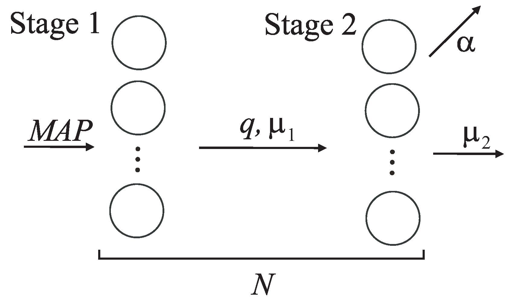
2. Mathematical Model

We consider the process of order delivery and picking up as a service in a tandem queueing system consisting of two stages. The structure of the system is shown in Figure 1.

Each client’s order has to be delivered to the pick-up point and then be issued there to the client. It is supposed that the order in the process of delivery, before reaching the pick-up point, receives service at Stage 1 of the tandem. Stage 2 of the tandem describes the operation of the point of issuing the orders that are already delivered to the pick-up point and are ready to be received by clients.

The process of order arrival to the tandem system is modeled by the $MAP$ flow characterized with matrices $D_0$ and $D_1$ of a finite size $W,W\ge 1.$ This process is governed by the indecomposable Markov chain with continuous-time ${\nu }_t,t\ge 0,$ with a state space $\{1,2,\dots ,W\}$, where W is a finite integer. The entries of the matrix $D_1$ are the intensities of transitions of the chain ${\nu }_t$ accompanied by an order arrival. The non-diagonal entries of the matrix $D_0$ determine the intensity of the corresponding transitions of the chain ${\nu }_t$ within its state space without an order arrival. The modules of the negative diagonal elements of the matrix $D_0$ determine the intensity of the departure of the process ${\nu }_t$ from the respective state. The matrix $D\left(1\right)=D_0+D_1$ is the irreducible generator of the Markov chain ${\nu }_t.$ The mean order arrival rate $\lambda$ is calculated as $\lambda =\theta D_1\mathbf{e}.$ Here, the row vector $\theta$ defines the stationary probabilities of the Markov chain ${\nu }_t$ and satisfies the system $\theta D\left(1\right)=\mathbf{0},\theta \mathbf{e}=1.$ Here and below, $\mathbf{0}$ is a row vector of a suitable size consisting of zeros, and $\mathbf{e}$ is a column vector of a suitable size consisting of ones.

As was already mentioned above, the significant advantage of the $MAP$ over other models of arrival flow, in particular the very popular model in the existing literature of the stationary Poisson process, is its suitability for fitting real-world flows with a wide range of the values of coefficients of variation and correlation of inter-arrival times. The problem of fitting the real-world arrival processes by the $MAP$ is addressed in many papers; see, e.g., [28,40,41,42,43,44].

Since the capacity of the warehouse at the pick-up point is limited, we assume that Stage 2 cannot provide service (storage until issuing to the client) to more than $N_2$ orders at the same time.

Generally speaking, the number of orders residing in the considered tandem system can be unlimited. However, if the number of orders accepted for service at Stage 1 is too large, then there is a high risk that the delivered order will not be accepted by the pick-up point due to the exhausted capacity of its warehouse and will be lost (or returned to a sender). To reduce the probability of this event, we apply order admission control. To this end, we fix an integer number $N,$ called threshold, such that $N>N_2,$ and assume that the tandem system temporarily terminates the acceptance of orders at Stage 1 when there are N orders residing at Stages 1 and 2 together. Thus, Stage 1 has a non-fixed maximum number of orders, which can be admitted. This number depends on the number of orders currently receiving service at Stage 2. It is worth noting that the real-world systems described by the considered model are highly computerized, and each arrival or withdrawal of an order at a pick-up point is registered immediately and automatically. Therefore, information about the current number of orders residing at Stages 1 and 2 together is permanently available for the order dispatcher.

When the number of orders residing in the system at a new order arrival moment is less than $N,$ the new order is admitted into the system and starts service, and the number of orders at Stage 1 increases by one. Otherwise, the arriving order is lost.

Because the transfer of orders from Stage 1 to Stage 2 in real-world prototypes of the considered tandem is usually performed in groups (by cars or trucks), we suggest the following mechanism of order transfer between the stages: Transfers can occur at random moments. The time distance between successive transfer moments is exponentially distributed with the parameter ${\mu }_1,{\mu }_1>0.$ At the transfer moment, each order staying at Stage 1 joins the group, which is transferred to Stage 2, with the probability $q,0<q\le 1,$ independently of other orders. Therefore, if the number of orders at Stage 1 is equal to $n,$ then the size of the group that transfers to Stage 2 is equal to l with the probability $C_n^l{q}^l{(1-q)}^{n-l},l=\overline{0,n}.$ Hereafter, a notation like $l=\overline{0,n}$ means that the parameter l admits the values from the set $\{0,1,\cdots ,n\}.$ If, at the time of the implementation of the transfer of l orders to Stage 2, there is enough space to place only $k,0\le k<l,$ orders there, then k orders are accepted at Stage 2 (to the warehouse of the pick-up point), and the remaining $l-k$ orders are lost.

We assume that each client of the tandem system (a person who places orders and has to obtain the corresponding goods at the warehouse of the pick-up point) can pick up several orders at once. Let the maximum number of orders available to a client be equal to $L.$ Then, each client obtains l orders from the pick-up point with the known probability $a_l,l=\overline{1,L},{\displaystyle \sum _{l=1}^L}{a}_l=1,$ if at the moment there are at least L orders in the warehouse. If there are only $m,m<L,$ orders in the warehouse of the pick-up point, then the client picks up l orders with the probability $a_l^{\left(m\right)},l=\overline{1,m},{\displaystyle \sum _{l=1}^m}{a}_l^{\left(m\right)}=1.$

The storage time of orders at the warehouse of Stage 2 is limited and has an exponential distribution with the parameter $\alpha ,\alpha \ge 0.$

There are two types of clients. The first type of clients is irresponsible. The clients of this type receive their orders only when the order’s storage time is completed. The second type of clients are responsible clients. They pick up their orders before the storage time of one of their orders is complete.

We assume that responsible clients pick up their orders after an exponentially distributed amount of time with the parameter ${\mu }_2,{\mu }_2>0.$ When the storage time expires, with the probability $1-p,0\le p\le 1,$ any client picks up all their orders (the order service is assumed to be finished), and with a complementary probability, the order, whose storage time is expired, is lost or is returned to a sender.

The main purpose of this research is to provide the opportunity for calculating the optimal capacity $N_2$ of the warehouse’s storage capacity and the threshold number N defining when the admission of new orders has to be postponed.

The problem of the optimal selection of N and $N_2$ is not trivial. A larger value of $N_2$ leads to the potential increase in the delivery system throughput; however, it requires greater expenses for more capacious warehouse maintenance or leasing. Moreover, the throughput may be sometimes more essentially influenced by the order arrival rate and storage time but not by the warehouse capacity. A too-small value of $N_2$ can lead to quick warehouse overloading, with frequent orders being delivered back and, as a consequence, the decision of a seller or a client to restrict the use of this pick-up point. A too-small value of the threshold N means the too strict limitation of order admission, which leads to the possible starvation of the pick-up point (and a decrease in the throughput). A too-large value of the threshold N leads to an increase in the probability that the admitted order cannot be accepted at the pick-up point and must be lost or sent back. Therefore, the parameters N and $N_2$ have to be chosen carefully and matched to each other to guarantee the best quality of the pick-up point operation.

3. The Process of System States and the Generator

Let the parameters N and $N_2$ be fixed:

$n_t^{\left(1\right)}$ is the number of orders residing at Stage 1, $n_t^{\left(1\right)}=\overline{0,N},$

$n_t^{\left(2\right)}$ is the number of orders residing at Stage 2, $n_t^{\left(2\right)}=\overline{0,\min \{N-n_t^{\left(1\right)},N_2\}},$

${\nu }_t$ is the state of the underlying process of the $MAP,$ ${\nu }_t=\overline{1,W},$

at time $t,t\ge 0.$

The behavior of the system under study is described by a regular irreducible continuous-time Markov chain:

$${\xi }_t=\{n_t^{\left(1\right)},n_t^{\left(2\right)},{\nu }_t\},t\ge 0.$$

Let us renumber the states of this chain in the direct lexicographical order of the components $\{n_t^{\left(1\right)},n_t^{\left(2\right)},{\nu }_t\}$ and call the set of states of the chain with the value n of the first component of the Markov chain level $n,n=\overline{0,N}.$ The set of states of the chain with the values $(n^{\left(1\right)},n^{\left(2\right)})$ of the first and second components of the Markov chain is called macrostate $(n^{\left(1\right)},n^{\left(2\right)}),n^{\left(1\right)}=\overline{0,N},n^{\left(2\right)}=\overline{0,\min \{N-n^{\left(1\right)},N_2\}}.$

Theorem 1.

The generator G of the Markov chain ${\xi }_t,t\ge 0,$ is a block lower Hessenberg matrix:

$$G=\left(\begin{array}{cccccccc}{G}_{0,0}& G_{0,1}& O& O& O& \dots & O& O\\ G_{1,0}& G_{1,1}& G_{1,2}& O& O& \dots & O& O\\ G_{2,0}& G_{2,1}& G_{2,2}& G_{2,3}& O& \dots & O& O\\ G_{3,0}& G_{3,1}& G_{3,2}& G_{3,3}& G_{3,4}& \dots & O& O\\ ⋮& ⋮& ⋮& ⋮& ⋮& \ddots & ⋮& ⋮\\ G_{N-1,0}& G_{N-1,1}& G_{N-1,2}& G_{N-1,3}& G_{N-1,4}& \dots & G_{N-1,N-1}& G_{N-1,N}\\ G_{N,0}& G_{N,1}& G_{N,2}& G_{N,3}& G_{N,4}& \dots & G_{N,N-1}& G_{N,N}\end{array}\right)$$

(1)

where the non-zero blocks $G_{n,n^{\prime }},n=\overline{0,N},n^{\prime }=\overline{0,min\{n+1,N\}},$ containing the intensities of transitions from level n to level $n^{\prime }$, are defined as follows:

$$\begin{gathered} G_{n,n}=I_{N_2+1}\otimes D_0-(1-{(1-q)}^n){\mu }_1{I}_{(N_2+1)W}-(\alpha +{\mu }_2)B_{N_2}\otimes I_W \\ +({\mu }_2+(1-p)\alpha )B_{N_2}{A}_{N_2}\otimes I_W+p\alpha B_{N_2}{F}_{N_2}\otimes I_W,n=\overline{0,N-N_2-1}, \end{gathered}$$

(2)

$$\begin{gathered} G_{n,n}=I_{N-n+1}\otimes D_0+{\widehat{I}}_{N-n}\otimes D_1-(1-{(1-q)}^n){\mu }_1{I}_{(N-n+1)W}-(\alpha +{\mu }_2)B_{N-n}\otimes I_W \\ +({\mu }_2+(1-p)\alpha )B_{N-n}{A}_{N-n}\otimes I_W+p\alpha B_{N-n}{F}_{N-n}\otimes I_W,n=\overline{N-N_2,N}, \end{gathered}$$

(3)

$$G_{n,n+1}=I_{N_2+1}\otimes D_1,n=\overline{0,N-N_2-1},$$

(4)

$$G_{n,n+1}=U_{N-n}\otimes D_1,n=\overline{N-N_2,N-1},$$

(5)

$$G_{n,n-n^{\prime }}=C_n^{n^{\prime }}{q}^{n^{\prime }}{(1-q)}^{n-n^{\prime }}{\mu }_1{E}^{\min \{n^{\prime },N_2\}}\otimes I_W,n=\overline{1,N-N_2},n^{\prime }=\overline{1,n},$$

(6)

$$G_{n,n-n^{\prime }}=C_n^{n^{\prime }}{q}^{n^{\prime }}{(1-q)}^{n-n^{\prime }}{\mu }_1{H}_{N-n,\min \{n^{\prime },N_2\}}\otimes I_W,n=\overline{N-N_2+1,N},n^{\prime }=\overline{1,n}.$$

(7)

Here, the following is true:

⊗ and ⊕ are the symbols of the Kronecker product and sum of matrices; see, for example, [45].

I is the identity matrix, and O is the zero matrix, the dimension of which is indicated by a subscript if necessary.

${\widehat{I}}_n$ is a square matrix of size $n+1$ with all zero elements except the element ${\left({\widehat{I}}_n\right)}_{n,n}=1,n=\overline{0,N_2}$.

$B_n$ is the diagonal matrix with the diagonal entries $\{0,1,2,\cdots ,n\},n=\overline{0,N_2}$.

$A_n$ is a square matrix of size $n+1$ with all zero elements except the elements ${\left(A_n\right)}_{m,m-l}=a_l^{\left(m\right)}$, $m=\overline{1,\min \{n,L-1\}},l=\overline{1,m},$ ${\left(A_n\right)}_{m,m-l}=a_l,m=\overline{L,n},l=\overline{1,L},$ and $n=\overline{0,N_2}.$

$F_n$ is a square matrix of size $n+1$ with all zero elements except the elements ${\left(F_n\right)}_{k,k-1}=1$, $k=\overline{1,n-1},$ and $n=\overline{0,N_2}.$

$U_n$ is a matrix of size $(n+1)\times n$ with all zero elements except the elements ${\left(U_n\right)}_{k,k}=1$, $k=\overline{0,n-1},n=\overline{1,N_2}.$

E is a square matrix of size $N_2+1$ with all zero elements except the elements ${\left(E\right)}_{n,n+1}=1$, $n=\overline{0,N_2-1},$ and ${\left(E\right)}_{N_2,N_2}=1.$

$H_{n,n^{\prime }}$ is a matrix of size $(n+1)\times \min \{n+n^{\prime }+1,N_2+1\}$ with all zero elements except the elements ${\left(H_{n,n^{\prime }}\right)}_{k,\min \{k+n^{\prime },N_2\}}=1,k=\overline{0,n},n=\overline{0,N_2-1},n^{\prime }=\overline{1,N_2}.$

Proof. 

The theorem is proved by studying the intensities of all conceivable transitions of the Markov chain ${\xi }_t$ during an infinitesimal time period.

The block lower Hessenberg structure of the matrix G is explained as follows: Since orders enter the system one at a time, the matrices $G_{n,n^{\prime }},n,n^{\prime }=\overline{0,N},$ are zero matrices for all $n,n^{\prime }$ such that $n^{\prime }>n+1.$ As a consequence of the possibility of a group transfer of orders from Stage 1 to Stage 2, the value n of the number of orders residing at Stage 1 can decrease during an infinitesimal time to any value of $n^{\prime }$ such that $n^{\prime }\le n.$ This explains the block lower Hessenberg structure (1) of the generator $G.$

Now, let us explain the form of all non-zero blocks $G_{n,n^{\prime }},0\le n^{\prime }\le \min \{N,n+1\}$, $n=\overline{0,N},$ of the generator.

Let us start with an explanation of forms (2) and (3) for the diagonal blocks $G_{n,n}$, $n=\overline{0,N}.$ Because the second component of the Markov chain ${\xi }_t$ cannot increase without the decrease in the first component, while it can decrease due to order withdrawal at Stage 2, the matrix $G_{n,n}$ has a block lower triangular structure.

All diagonal elements of the block $G_{n,n}$ are negative, and the absolute values of these elements determine the intensities of the Markov chain ${\xi }_t,t\ge 0,$ exiting the corresponding states. The Markov chain ${\xi }_t,t\ge 0$ can exit the current state in the following cases:

(1) The underlying process ${\nu }_t,t\ge 0$ of order arrivals leaves its current state. The corresponding transition intensities are determined up to sign by the diagonal elements of the matrix $I_{\min \{N-n,N_2\}+1}\otimes D_0.$ Note that if the system already has N orders and the underlying process makes a transition to the same state with the generation of a new order, then this generated order is lost and there is no exit from the current state. This is taken into account by adding diagonal elements of matrices ${\widehat{I}}_{N-n}\otimes D_1$ to the diagonal elements of the blocks $G_{n,n}$ for $n=\overline{N-N_2,N}.$

(2) A moment of order transfer to Stage 2 occurs, and at least one order moves to this stage. In this case, the transition intensities are determined by the elements of the matrix $(1-{(1-q)}^n){\mu }_1{I}_{(\min \{N-n,N_2\}+1)W}.$

(3) The order storage time expires. The matrix $\alpha B_{\min \{N-n,N_2\}}\otimes I_W$ defines the corresponding transition intensities.

(4) A client comes to the pick-up point and picks up their orders. The corresponding transition intensities are specified by the matrix ${\mu }_2{B}_{\min \{N-n,N_2\}}\otimes I_W.$

The non-diagonal elements of the matrix $G_{n,n}$ define the transition intensities of the Markov chain ${\xi }_t$ without changing the value n of the first component. These transitions are given by the following:

(1) Non-diagonal elements of matrices $I_{\min \{N-n,N_2\}+1}\otimes D_0$ when the underlying process ${\nu }_t$ makes a transition without generating an order.

(2) Non-diagonal elements of the matrix ${\widehat{I}}_{N-n}\otimes D_1,n=\overline{N-N_2,N},$ when the underlying process ${\nu }_t$ makes a transition, generating an order that is lost due to the presence of N orders in the tandem system.

(3) Elements of the matrix ${\mu }_2{B}_{\min \{N-n,N_2\}}{A}_{\min \{N-n,N_2\}}\otimes I_W$ when a responsible client picks up their orders.

(4) Elements of the matrix $(1-p)\alpha B_{\min \{N-n,N_2\}}{A}_{\min \{N-n,N_2\}}\otimes I_W$ when the order, whose storage time is expired, is lost (returned from the warehouse to the seller).

(5) Elements of the matrix $p\alpha B_{\min \{N-n,N_2\}}{F}_{\min \{N-n,N_2\}}\otimes I_W$ when the storage time is expired but an irresponsible client picks up all their orders.

Thus, we obtain forms (2) and (3) of blocks $G_{n,n},n=\overline{0,N}.$

Forms (4) and (5) of the blocks $G_{n,n+1},n=\overline{0,N-1},$ are explained as follows: These blocks contain the transition rates of the Markov chain ${\xi }_t,t\ge 0,$ when the number of orders at Stage 1 increases by one. This is only possible in the case of a new order arrival to the tandem system. The number of orders at Stage 2 does not change at this arrival moment. Therefore, the matrix $G_{n,n+1}$ is block diagonal. The elements of the matrix $D_1$ determine the transition intensities of the process ${\nu }_t,t\ge 0,$ at the time of the order’s arrival.

Thus, the blocks $G_{n,n+1}$ are defined by the matrices of form (4) for $n=\overline{0,N-N_2-1}$ and (5) for $n=\overline{N-N_2,N-1}.$

The blocks $G_{n,n-n^{\prime }}$ of the generator $G,n=\overline{1,N},n^{\prime }=\overline{1,n}$ contain the transition intensities of the Markov chain ${\xi }_t,t\ge 0$ from a state with value n of the first component of the chain to a state with the value $n-n^{\prime }$ of this component in the case when a group of orders of size $n^{\prime }$ is sent to Stage 2 (the warehouse of the pick-up point). The number of customers at Stage 2 increases. Therefore, the matrix $G_{n,n-n^{\prime }}$ is block upper triangular. These intensities are determined by the matrix $C_n^{n^{\prime }}{q}^{n^{\prime }}{(1-q)}^{n-n^{\prime }}{\mu }_1{E}^{\min \{n^{\prime },N_2\}}\otimes I_W$ for $n=\overline{1,N-N_2}$ and by the matrix $C_n^{n^{\prime }}{q}^{n^{\prime }}{(1-q)}^{n-n^{\prime }}{\mu }_1{H}_{N-n,\min \{n^{\prime },N_2\}}\otimes I_W$ if $n=\overline{N-N_2+1,N}.$ Thus, formulas (6) and (7) are valid. The theorem is proven. □

Because the Markov chain ${\xi }_t,t\ge 0$ is irreducible and has a finite state space, for any values of the system parameters, there are the stationary probabilities of the states of this Markov chain:

$$\pi (n,n^{\prime },\nu )=\underset{t\to \infty }{lim}P\{n_t^{\left(1\right)}=n,n_t^{\left(2\right)}=n^{\prime },{\nu }_t=\nu \},$$

$$n=\overline{0,N},n^{\prime }=\overline{0,\min \{N-n,N_2\}},\nu =\overline{1,W}.$$

Let us form the row vectors $\pi (n,n^{\prime }),n=\overline{0,N},n^{\prime }=\overline{0,\min \{N-n,N_2\}}$ of the stationary probabilities of the states belonging to the macrostate $(n,n^{\prime })$ and the vectors ${\mathit{\pi }}_n=(\mathit{\pi }(n,0),\mathit{\pi }(n,1),\cdots ,\mathit{\pi }(n,\min \{N-n,N_2\}))$ of the stationary probabilities of the states belonging to the level $n,n=\overline{0,N}.$

It is well known that the row vectors ${\mathit{\pi }}_n,n=\overline{0,N}$ satisfy the following system of equilibrium equations:

$$({\mathit{\pi }}_0,{\mathit{\pi }}_1,\cdots ,{\mathit{\pi }}_N)G=\mathbf{0},({\mathit{\pi }}_0,{\mathit{\pi }}_1,\cdots ,{\mathit{\pi }}_N)G\mathbf{e}=1.$$

(8)

Because the matrix G does not have a block tridiagonal structure, the Markov chain ${\xi }_t$ does not belong to the class of the finite state Quasi-Birth-and-Death processes, as discussed in [21], so its solution is not trivial, especially in the case of the large size of the generator $G.$ This size can indeed be very large in real-world applications when the capacity of the warehouse at the pick-up point is large. The system of equilibrium equations can be solved using the numerically stable algorithms recently offered in [46]. These algorithms effectively account for the block lower Hessenberg structure of the generator $G.$

Therefore, the flowchart of the computation of the row vectors ${\mathit{\pi }}_n,n=\overline{0,N}$ of the stationary distribution of the Markov chain ${\xi }_t$ is as follows:

• Compute the matrices $G_{n,n},n=\overline{0,N},G_{n,n+1},n=\overline{0,N-1},G_{n,n-n^{\prime }}n=\overline{1,N}$, $n^{\prime }=\overline{1,n},$ by formulas (2)–(7);
• Compute the generator G by formula (1);
• Compute vectors ${\mathit{\pi }}_n,n=\overline{0,N}$ as the unique solution of the system (8).

The knowledge of the stationary distribution of the Markov chain ${\xi }_t$ allows us to evaluate the values of various performance measures of the considered tandem system under any fixed values for the system parameters, including the threshold N and the capacity $N_2.$

4. Performance Measures

The mean number of orders receiving service at Stage 1 at an arbitrary moment is calculated as

$$L^{\left(1\right)}=\sum _{n=1}^{N}n{\mathit{\pi }}_n\mathbf{e}.$$

(9)

The average number of orders transferred to Stage 2 during an arbitrary transfer moment is calculated as

$$K^{\left(1\right)}=q{L}^{\left(1\right)}.$$

The mean number of orders receiving service at Stage 2 at an arbitrary moment is calculated as

$$L^{\left(2\right)}=\sum _{n=0}^{N-1}\sum _{n^{\prime }=1}^{\min \{N-n,N_2\}}{n}^{\prime }\mathit{\pi }(n,n^{\prime })\mathbf{e}.$$

(10)

The mean number of orders receiving service in the tandem at an arbitrary moment is calculated as

$$L^{\left(tandem\right)}=\sum _{n=0}^N\sum _{n^{\prime }=0}^{\min \{N-n,N_2\}}(n+n^{\prime })\mathit{\pi }(n,n^{\prime })\mathbf{e}=L_1+L_2.$$

The rate of the output flow of orders from Stage 1 is calculated as

$${\lambda }_{out}^{\left(1\right)}=\sum _{n=1}^N\sum _{m=1}^{n}m{C}_n^m{q}^m{(1-q)}^{n-m}{\mu }_1{\mathit{\pi }}_n\mathbf{e}={\mu }_1{K}^{\left(1\right)}.$$

The rate of the output flow of serviced orders from Stage 2 is calculated as

$${\lambda }_{out}^{\left(2\right)}=({\mu }_2+(1-p)\alpha )\sum _{n=0}^{N-1}(\sum _{n^{\prime }=1}^{\min \{N-n,L-1\}}{n}^{\prime }\sum _{l=1}^{n^{\prime }}l{a}_l^{\left(n^{\prime }\right)}\mathit{\pi }(n,n^{\prime })\mathbf{e}+$$

$$\sum _{n^{\prime }=L}^{\min \{N-n,N_2\}}{n}^{\prime }\sum _{l=1}^{L}l{a}_l\mathit{\pi }(n,n^{\prime })\mathbf{e}).$$

The average number of orders picked up by an arbitrary client at Stage 2 is calculated as

$$K^{\left(2\right)}=\sum _{n=0}^{N-1}\left(\sum _{n^{\prime }=1}^{\min \{N-n,L-1\}}\sum _{l=1}^{n^{\prime }}l{a}_l^{\left(n^{\prime }\right)}\mathit{\pi }(n,n^{\prime })\mathbf{e}+\sum _{n^{\prime }=L}^{\min \{N-n,N_2\}}\sum _{l=1}^{L}l{a}_l\mathit{\pi }(n,n^{\prime })\mathbf{e}\right).$$

The loss probability of an order at the entrance at Stage 1 is calculated as

$$P_{ent}^{\left(1\right)}={\displaystyle \frac{1}{\lambda }}\sum _{n=N-N_2}^N\mathit{\pi }(n,N-n)D_1\mathbf{e}.$$

The loss probability of an order at the entrance at Stage 2 is calculated as

$$P_{ent}^{\left(2\right)}={\displaystyle \frac{1}{\lambda }}\sum _{n=1}^N\sum _{n^{\prime }=\max \{0,N_2-n+1\}}^{\min \{N_2,N-n\}}\sum _{l=N_2-n^{\prime }+1}^n{C}_n^l{q}^l{(1-q)}^{n-l}(l-(N_2-n^{\prime })){\mu }_1\mathit{\pi }(n,n^{\prime })\mathbf{e}.$$

(11)

The loss probability of an order due to a recipient no-show before the expiration of the storage time at Stage 2 is calculated as

$$P_{imp}^{\left(2\right)}={\displaystyle \frac{1}{\lambda }}\sum _{n=0}^{N-1}\sum _{n^{\prime }=1}^{\min \{N-n,N_2\}}p{n}^{\prime }\alpha \mathit{\pi }(n,n^{\prime })\mathbf{e}={\displaystyle \frac{p\alpha L^{\left(2\right)}}{\lambda }}.$$

The loss probability of an arbitrary order can be calculated as

$$P_{loss}=P_{ent}^{\left(1\right)}+P_{ent}^{\left(2\right)}+P_{imp}^{\left(2\right)}=1-{\displaystyle \frac{{\lambda }_{out}^{\left(2\right)}}{\lambda }}.$$

The latter equality can be used for the verification of the correctness of the computation of the stationary distribution of the Markov chain ${\xi }_t.$

Let us comment briefly on the derivation of formulas (9)–(11). Formula (9) defines the expectation of the number of orders receiving service at Stage 1, which is a discrete random variable with a probability distribution ${\mathit{\pi }}_n\mathbf{e},n=\overline{0,N}.$ Formula (10) defines the expectation of the number of orders receiving service at Stage 2, which is a discrete random variable with a probability distribution ${\displaystyle \sum _{n=0}^{N-1}}\mathit{\pi }(n,n^{\prime })\mathbf{e},n^{\prime }=\overline{0,N}.$ Formula (11) for loss probability $P_{ent}^{\left(2\right)}$ is evident because this probability is the ratio of two rates. The first one is the rate of the lost orders, i.e., the orders that finished service at Stage 1 when the numbers of orders at Stage 1 and Stage 2 are n and $n^{\prime },$ correspondingly, $n=\overline{1,N}$, $n^{\prime }=\overline{\max \{0,N_2-n+1\},\min \{N_2,N-n\}},$ in a batch of size l such that $N_2-n^{\prime }+1\le l\le n$ and did not have the luck to be among $N_2-n^{\prime }$ customers that are accepted to Stage 2 and, therefore, are lost. The formula of the total probability is used for the calculation of this rate. The second one is the total rate $\lambda$ of order arrival to the tandem. Other formulas for performance measures are explained similarly.

5. Numerical Examples

The aim of this section is to present the numerical results that highlight the dependence of some performance measures of the system on the parameters N and $N_2$ and to demonstrate the possibility of using the obtained results for managerial goals.

It is assumed that orders enter the tandem system in the $MAP$ flow defined by the matrices

$$D_0=\left(\begin{array}{cc}-3& 0\\ 0& -0.9\end{array}\right),D_1=\left(\begin{array}{cc}2.91& 0.09\\ 0.03& 0.87\end{array}\right).$$

This $MAP$ has the average arrival rate $\lambda =1.425,$ the coefficient of correlation of successive inter-arrival times $c_{cor}=0.177894$, and the coefficient of variation in inter-arrival times $c_{var}=1.6125.$

We assume that the rate of order transfer to the pick-up point is ${\mu }_1=0.2$, the rate of orders received by responsible clients is ${\mu }_2=0.03$, and the rate of the storage time expiration is $\alpha =0.003$. The probabilities p and q are defined as $p=0.1$ and $q=0.12.$

Let the maximum number of orders available for receipt by an arbitrary client be equal to $L=5.$

We assume that each client receives $l,l=\overline{1,5}$ orders from the pick-up point with the probabilities $a_l,l=\overline{1,5},$ defined as $a_1=0.4,a_2=0.3,a_3=0.2,a_4=0.05,a_5=0.05,$ if there are at least five orders in the warehouse. Otherwise, the client picks up l orders with the probabilities defined as $a_l^{\left(m\right)}={\displaystyle \frac{a_l}{{\displaystyle \sum _{k=1}^m}{a}_k}},l=\overline{1,m},m=\overline{1,4}.$

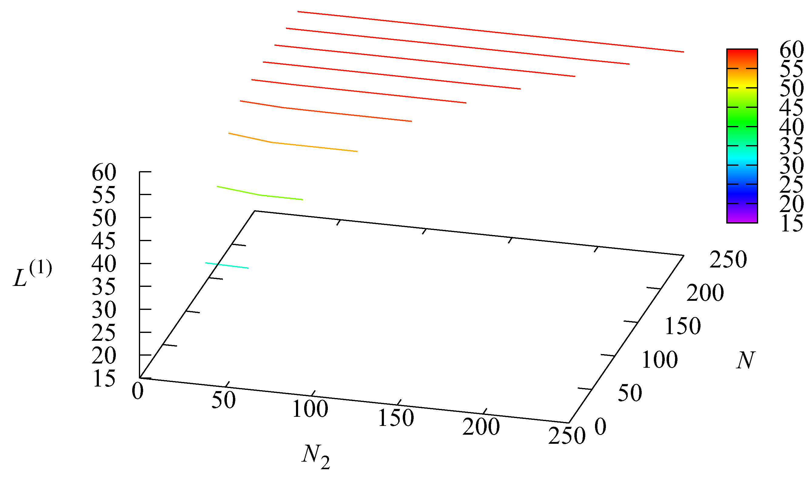
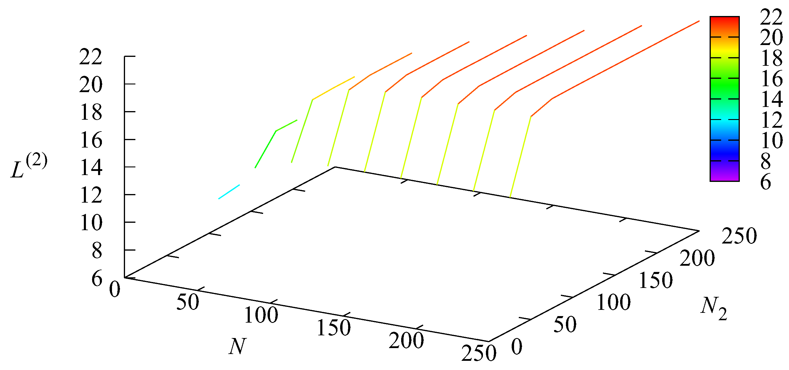
Let us vary the maximum number N of orders, which can stay in the tandem system simultaneously, in the range from 25 to 250 and the maximum number $N_2$ of orders at Stage 2 in the range from 25 to N with step 25.

Figure 2 and Figure 3 illustrate the dependencies of the mean number of orders $L^{\left(1\right)}$ and $L^{\left(2\right)}$ at Stage 1 and Stage 2, respectively, on the values of the parameters N and $N_2.$

The value of $L^{\left(1\right)}$ quickly increases when the limiting value N of orders that can reside in the system at the same time increases. The increase practically stops after N reaches the value 150. The value of $L^{\left(1\right)}$ weakly depends on the values of $N_2.$ It only slightly decreases with the growth of $N_2.$ The value of $L^{\left(2\right)}$ increases with the increase in N (more orders are admitted to the system and can be stored in the warehouse) and quickly increases with the growth of $N_2$ (more orders are stored in the warehouse when its capacity becomes larger). However, the increase becomes slow for $N_2$ greater than 75.

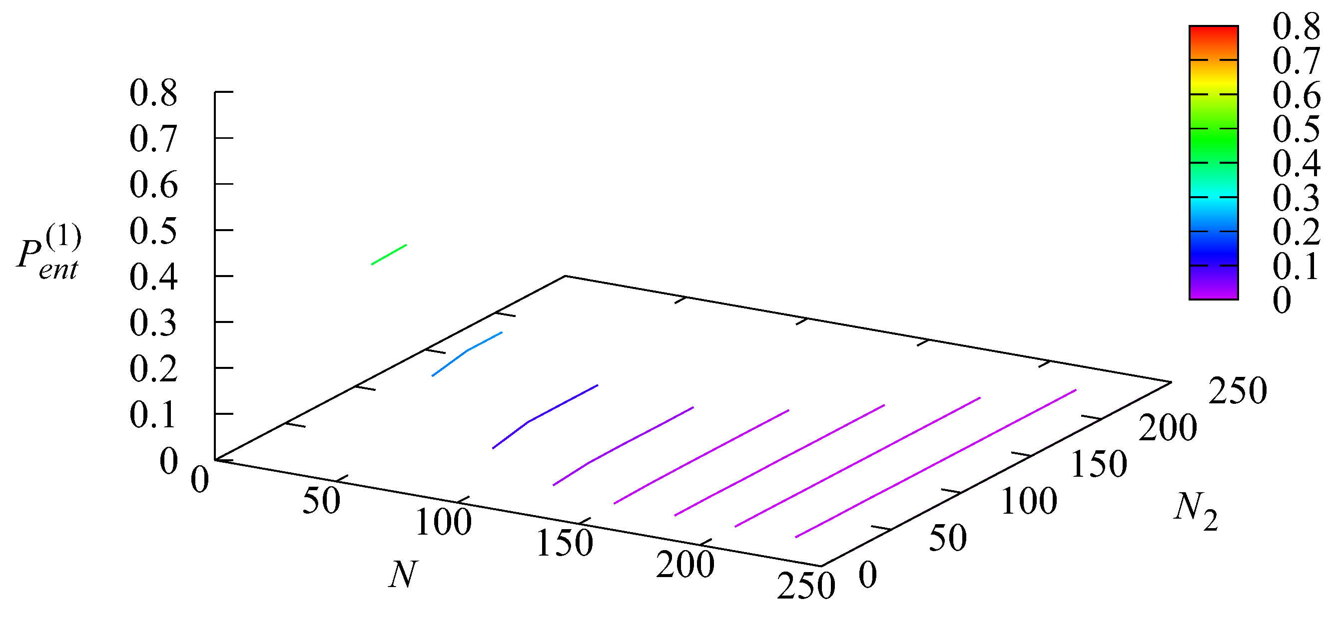
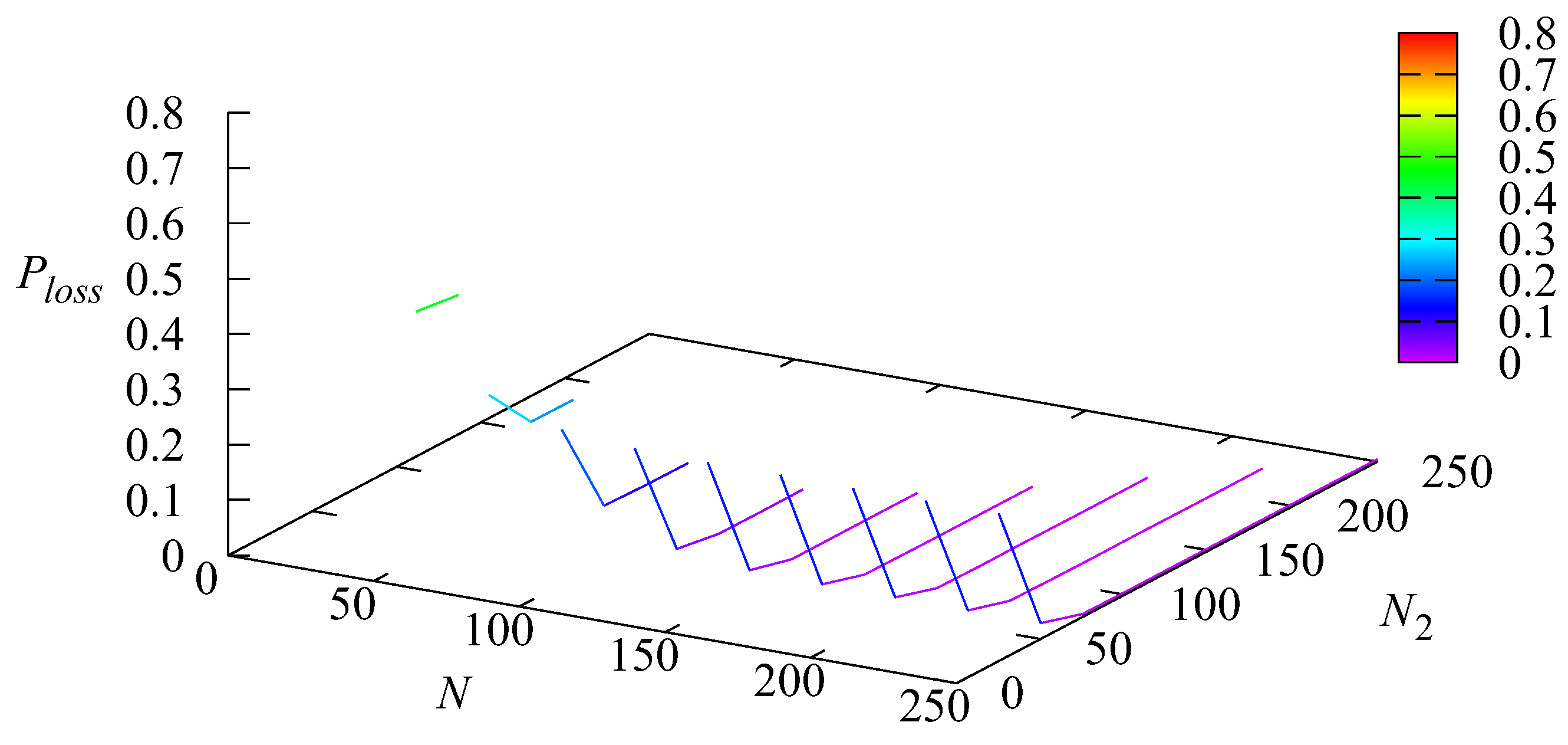
Figure 4 and Figure 5 show the dependencies of the loss probability $P_{ent}^{\left(1\right)}$ of an order at the entrance at Stage 1 and the loss probability $P_{ent}^{\left(2\right)}$ at the entrance at Stage 2 on the parameters N and $N_2.$

The loss probability $P_{ent}^{\left(1\right)}$ is very large for small values of N (around 0.7 for $N=25$) and quickly decreases (and becomes weakly dependent on $N_2$) when N increases. For $N=175+25k,k\ge 0,$ this probability is in the order of ${10}^{-3-k}.$ The loss probability $P_{ent}^{\left(2\right)}$ obviously is equal to zero when $N_2=N,$ i.e., any order is not admitted to Stage 1 if Stage 2 is full. This probability grows with the increase in N but decreases very quickly with the increase in $N_2.$

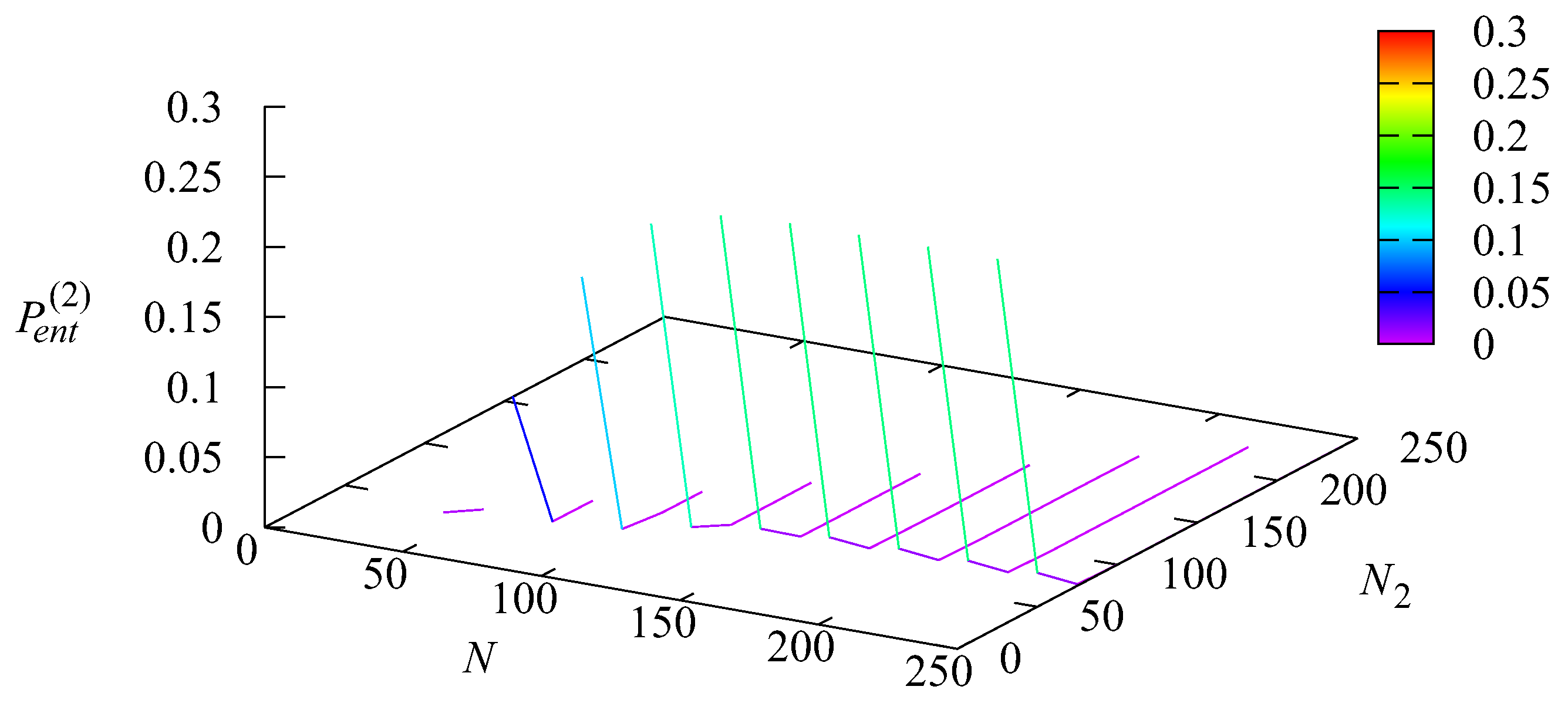
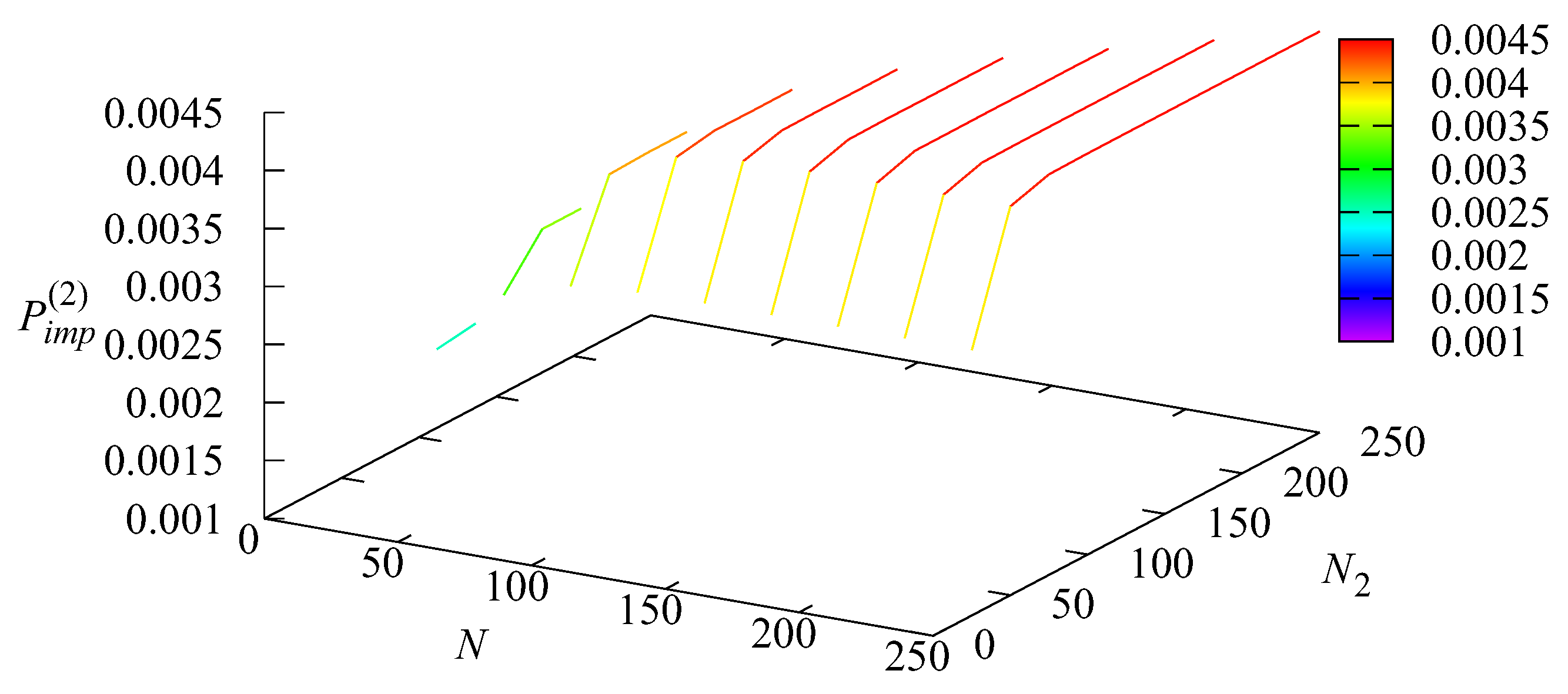
The dependencies of the loss probability $P_{imp}^{\left(2\right)}$ of an order due to client no-show at Stage 2 and the loss probability of an arbitrary order $P_{loss}$ are presented in Figure 6 and Figure 7.

The loss probability $P_{imp}^{\left(2\right)}$ is expectably small when the capacity $N_2$ of the warehouse is small and increases with the increase in $N_2.$ It becomes stable (around 0.004) after $N_2$ reaches the value 50 for $N\ge 100.$

Because the loss probability of an arbitrary order $P_{loss}$ is the sum of the loss probabilities $P_{ent}^{\left(1\right)},$$P_{ent}^{\left(2\right)},$ and $P_{imp}^{\left(2\right)},$ the shape of the surface presented in Figure 7 matches Figure 4, Figure 5 and Figure 6.

Table 2. The values of some performance measures of the system for certain values of the parameters N and $N_2$.

Performance     Measure	$\mathit{N}=25$${\mathit{N}}_2=25$	$\mathit{N}=50$${\mathit{N}}_2=25$	$\mathit{N}=50$${\mathit{N}}_2=50$	$\mathit{N}=75$${\mathit{N}}_2=25$	$\mathit{N}=75$${\mathit{N}}_2=50$	$\mathit{N}=75$${\mathit{N}}_2=75$
$L^{\left(1\right)}$	17.56	33.79	33.63	46.83	45.91	45.91
$L^{\left(2\right)}$	6.38	11.81	12.02	14.51	16.38	16.38
$P_{ent}^{\left(1\right)}$	0.704	0.431	0.434	0.211	0.227	0.227
$P_{ent}^{\left(2\right)}$	0	0.013	0	0.104	$6\times {10}^{-5}$	0
$P_{imp}^{\left(2\right)}$	0.001	0.002	0.003	0.003	0.003	0.003

supplements the results of calculations presented for this example in graphical form by presenting the concrete values of $L^{\left(1\right)}$, $L^{\left(2\right)}$, $P_{ent}^{\left(1\right)}$, $P_{ent}^{\left(2\right)}$, and $P_{imp}^{\left(2\right)}$ for some values of the parameters N and $N_2$.

With the algorithms and software, which allowed us to clarify the dependence of the key performance measures of the system on the controlled parameters, it is possible to formulate various criteria of system operation and solve the optimization problems. The most popular in the literature is the criterion that counts the revenue of the system earned via service provisioning, possible expenditures of the system related to the different reasons for the loss of some orders, and the cost of system equipment maintenance.

For example, let us choose the following cost criterion for the evaluation of the system’s operation quality:

$$J=J(N,N_2)=c_1{\lambda }_{out}^{\left(2\right)}-c_2\lambda P_{ent}^{\left(1\right)}-c_3\lambda P_{ent}^{\left(2\right)}-c_4\lambda P_{imp}^{\left(2\right)}-c_5{N}_2$$

where $c_1$ is the average system’s profit obtained via one order service; $c_2$ and $c_3$ are the penalties for an order loss at the entrance at Stage 1 and Stage 2, respectively; $c_4$ is the penalty for an order loss due to the failure to receive goods by clients; and $c_5$ is the cost of using a unit of space for order storage at the warehouse.

Let us set the values of cost coefficients for this numerical example as follows:

$$c_1=3,c_2=3,c_3=50,c_4=0.1,c_5=0.01.$$

The cost $c_3$ is supposed to be the largest because the rejection of an order at Stage 2 due to a full warehouse implies not only the lost potential profit but also the expenditures related to order utilization or sending it back to a sender.

The dependence of the criterion J on the capacities N and $N_2$ is presented in Figure 8.

The values of the cost criterion for various values of N are presented in

Table 3. Values of $J(N,N_2)$ for $N_2=25,N_2=N_2^{*}$, and $N_2=N$ for different values of N.

N	$\mathit{J}(\mathit{N},25)$	${\mathit{N}}_2^{*}$	$\mathit{J}(\mathit{N},{\mathit{N}}_2^{*})$	$\mathit{J}(\mathit{N},\mathit{N})$
25	−2.0025	25	−2.0025	−2.0025
50	−0.6516	50	0.0564	0.0564
75	−5.6568	50	1.8166	1.5710
100	−11.6094	75	2.6942	2.4442
125	−14.6455	75	3.2472	2.7508
150	−15.6008	75	3.4201	2.6967
175	−15.8122	75	3.4415	2.4949
200	−15.8487	75	3.4383	2.2538
225	−15.8541	75	3.4366	2.0051
250	−15.8548	75	3.4363	1.7552

. Each row of the table corresponds to a fixed value of N and contains the values of $J(N,N_2)$ for $N_2=25,N_2=N_2^{*}$, and $N_2=N$ where $N_2^{*}$ is the value of the parameter $N_2$ within the chosen grid that provides maximum to $J(N,N_2)$ for the given value of $N.$

One can see that the optimal (maximal) value of J is $3.44146$ and is reached for $N^{*}=175$ and $N_2=75.$ It is worth noting that the revenue is negative for any value of N when the warehouse capacity $N_2$ is small.

6. Conclusions

In this paper, we considered the mathematical model of order delivery to the client as processing in the dual tandem queue. Stage 1 of the tandem corresponds to the order’s generation, preparation for transportation, and delivery (probably within a whole batch of orders) to the pick-up point. Stage 2 corresponds to the order being received at the pick-up point, its storage in the warehouse, and its issue to the client (probably within a group of orders). The input flow is described by the quite general $MAP.$ The possibility of some clients not showing up is taken into account. The threshold strategy of an order’s admission to Stage 1 of the tandem to mitigate the possible negative effect of order rejection at Stage 2 due to warehouse overflow is proposed. Under the fixed value of the threshold, the stationary behavior of the system is analyzed via the consideration of the suitably constructed multidimensional Markov chain with the block lower Hessenberg structure of the generator. The presented numerical results confirm the feasibility of the proposed method for the computation of the key performance measures of the system and illustrate the potential usefulness of the results for managerial goals.

In this paper, we assumed that the clients receive their orders immediately after coming to the pick-up point. Indeed, due to the finite number of operators that issue the orders to the clients, the clients can spend a certain time in the queue. We assumes that this waiting time is negligible because this time is very small compared to, e.g., the transportation time and storage time at pick-up points. In the future, the considered model can be generalized to account for the possible waiting of clients in a queue due to the lack of self-service pick-up machines or the manual service desks for manual order processing. The single-stage queueing model of a pick-up point operation that accounts for this was considered in [20] algorithmically and in [47] via computer simulation. The results can also be extended to the cases of batch order generation at Stage 1 and phase-type distribution of order group transportation time to the pick-up point with irreducible representation dependent on the size of a group. The possibility of orders’ direct arrival to Stage 2 from other sources (so-called cross-traffic) could be taken into account as well.