Discrete-Time Retrial Queuing Systems with Last-Come-First-Served (LCFS) and First-Come-First-Served (FCFS) Disciplines: Negative Customer Impact and Stochastic Analysis

Abstract

This paper examines a discrete-time retrial queuing system that incorporates negative customers, system breakdowns, and repairs. In this model, an arriving customer has the option to go directly to the server, pushing the currently served customer, if any, to the front of the orbit queue, or to join the orbit based on a First-Come-First-Served (FCFS) discipline. The study also considers negative customers who not only remove the customer currently being served but also cause a server breakdown. An in-depth analysis of the model is conducted using a generating function approach, leading to the determination of the distribution and expected values of the number of customers in the orbit and the entire system. The paper explores the stochastic decomposition law and provides bounds for the difference between the steady-state distribution of this system and a comparable standard system. Recursive formulas for the steady-state distributions of the orbit and the system are developed. Additionally, it is shown that the studied discrete-time system can approximate the M/G/1 continuous-time version of the model. The research includes a detailed examination of the customer’s sojourn time distribution in the orbit and the system, utilizing the busy period of an auxiliary system. The paper concludes with numerical examples that highlight how different system parameters affect various performance characteristics, and a section summarizing the key research contributions.

1. Introduction

This queuing system with retrials and interruptions is motivated by the need to model real-life processes that involve dynamic and complex interactions between servers and customers. Its design captures behaviors such as customer retries, interruptions caused by negative arrivals, and server breakdown, making it a versatile tool for studying a wide range of systems.

The flexibility of this queuing system allows it to be applied across various fields. If we focus on manufacturing systems or call centers, in both contexts, tasks or customers may need to retry for processing after some delay. Negative arrivals, which cause breakdowns, can represent machine failures in production systems interrupting job processing, and technical issues in call centers or IT systems, temporarily halting operations.

The pioneering studies on retrial queues present the concept of classical retrial policy, wherein each of the blocked customers generates a stream of repeated attempts independent of the rest of the customers in the orbit. Such a type of retrial policy is investigated by [1,2]. If we consider a model with two orbits, we refer to [3], where a retrial queue system with these characteristics is analyzed. Finally, if the focus is on $BMAP/PH/N$ queuing systems with threshold-dependent inter-retrial time distributions, ref. [4] presents a methodology based on stochastic analysis for such scenarios.

Queues with a server subject to breakdown occur in flexible manufacturing systems and computer communication networks, and they heavily affect the performance of the systems. A retrial queuing system with server down and repair is considered in [5]. A general service time retrial queue with breakdown is analyzed in [6,7]. For systems with collisions, impatient customers, and unreliable servers, the asymptotic analysis presented in [8] provides a solid foundation for understanding these phenomena in $M/M/1$ systems. In the case of systems with controlled arrivals, essential interruptions, and emergency vacationing servers, the work in [9] offers a detailed approach for these types of queue–inventory systems.

In papers from the end of the 1980s and early 1990s, new models introduced the concept of “negative” or “positive” customers. The notion of negative customers was introduced by Gelenbe in the paper [10] with G-networks which can eliminate a positive or an ordinary customer if present. On the other hand, a geometric discrete-time queue with negative and positive customers appeared only a few decades after in the literature.

Harrison and Pitel [11] initially studied the $M/M/1$ queue incorporating both negative and positive customers. Their work was further expanded by the same authors [12] to include the $M/G/1$ queue, and Yang and Chae [13] extended it to the $GI/M/1$ queue. The concept of negative customers was explored in retrial queues by Artalejo and Gómez-Corral [14]. Chakka and Harrison [15] examined a Markov modulated multi-server queue with negative customers. Li and Zhao [16] analyzed a queuing model with negative customers under a Markovian arrival process (MAP). Additionally, Atencia and Moreno [17] provided an analysis of the time-average queue length distribution for a $Geo/Geo/1$ queue with negative and positive customers, under specific assumptions regarding the sequence of negative arrivals, positive arrivals, and service completions.

2. The Mathematical Model

Imagine a discrete-time single server retrial queue where the timeline is divided into equal intervals, known as slots. These intervals are denoted by $0,1,\dots ,m,\dots$. In this system, all queuing activities—such as arrivals, departures, retrials, and the start and end of repairs—are assumed to occur around the boundaries of these slots.

Specifically, at the time point m, departures and the end of repairs happen in the interval $(m^{-},m)$, while arrivals, the start of repairs, and retrials, in that sequence, take place in the interval $(m,m^{+})$.

If the server is busy and a customer enters the system, several scenarios may occur:

• With probability ${\theta }_0$, the customer leaves the service area and joins a group of unsatisfied customers called the orbit, following a First-Come-First-Served (FCFS) discipline.
• With probability ${\theta }_1$, the new customer replaces the customer currently being served, who is placed at the front of the orbit, and immediately begins their service.
• With probability ${\theta }_2$, the incoming customer becomes a negative customer. This negative customer not only removes the customer currently being served from the system but also causes a breakdown in the server, followed by a repair period that follows a general distribution ${\left\{r_i\right\}}_{i=1}^{\infty }$ with a generating function $R\left(x\right)={\sum }_{i=1}^{\infty }{r}_i{x}^i$. The negative customer causing the breakdown, after removing the customer being served, disappears from the system.

If the server is free when a customer arrives, the customer begins its service with probability $1-{\theta }_2$ or becomes a negative customer with probability ${\theta }_2$. In this case, negative customers have no effect on the system.

If the server is down, a customer arriving in the system joins the end of the orbit with probability $1-{\theta }_2$ or becomes a negative customer with probability ${\theta }_2$, having no effect on the system’s operation.

Let us note that only the customer at the front of the orbit can access the server. The time between retrials is defined by an arbitrary distribution ${\left\{a_i\right\}}_{i=0}^{\infty }$, with the generating function $A\left(x\right)={\sum }_{i=0}^{\infty }{a}_i{x}^i$. Service times are independent and identically distributed, following a general distribution ${\left\{s_i\right\}}_{i=1}^{\infty }$, represented by the generating function $S\left(x\right)={\sum }_{i=1}^{\infty }{s}_i{x}^i$. We define $S_k={\sum }_{i=k}^{\infty }{s}_i$ for $k\ge 1$, which represents the probability that the service duration is at least k slots.

3. The Markov Chain

Just after the end of time slot m (at time $m^{+}$), the system’s state is characterized by the process

$$X_m=(C_m,{\xi }_m,N_m).$$

In this model, the server’s status at time m is represented by $C_m$, where 0 indicates the server is free, 1 means it is busy, and 2 signifies it is under repair. The number of customers in the retrial queue is denoted by $N_m$. If $C_m=0$ and there are customers waiting ($N_m>0$), ${\xi }_m$ represents the remaining time until the next retrial attempt. When $C_m=1$, ${\xi }_m$ refers to the remaining service time for the current customer. Finally, if $C_m=2$, ${\xi }_m$ indicates the time left until the server repair is completed. Let as define $(0,0)$ as the state in which $C_m=N_m=0$.

Let us note note that $\{X_m,m\in \mathbf{N}\}$ is the Markov chain of our queuing system, whose state space is

$$\left\{\right(0,0);(0,i,k):i\ge 1,k\ge 1;(1,i,k):i\ge 1,k\ge 0;(2,i,k):i\ge 1,k\ge 0\}$$

Now, the objective is to obtain the stationary distribution

$$\begin{array}{ccc}\hfill {\pi }_{0,0}& =& \underset{m\to \infty }{lim}P[C_m=0,N_m=0],\hfill \\ \hfill {\pi }_{0,i,k}& =& \underset{m\to \infty }{lim}P[C_m=0,{\xi }_m=i,N_m=k];i\ge 1,k\ge 1,\hfill \\ \hfill {\pi }_{1,i,k}& =& \underset{m\to \infty }{lim}P[C_m=1,{\xi }_m=i,N_m=k];i\ge 1,k\ge 0,\hfill \\ \hfill {\pi }_{2,i,k}& =& \underset{m\to \infty }{lim}P[C_m=2,{\xi }_m=i,N_m=k];i\ge 1,k\ge 0.\hfill \end{array}$$

of the Markov chain $\{X_m,m\in \mathbf{N}\}$.

The system of equilibrium equations (SEE) that describes the stationary distribution can be expressed as

$$\begin{array}{ccc}\hfill {\pi }_{0,0}& =& (\overline{a}+a{\theta }_2)[{\pi }_{0,0}+{\pi }_{1,1,0}+{\pi }_{2,1,0}]\iff \hfill \\ \hfill a(1-{\theta }_2){\pi }_{0,0}& =& (\overline{a}+a{\theta }_2)({\pi }_{1,1,0}+{\pi }_{2,1,0})\hfill \end{array}$$

(1)

$$\begin{array}{ccc}\hfill {\pi }_{0,i,k}& =& (\overline{a}+a{\theta }_2)\left[{\pi }_{0,i+1,k}+a_i{\pi }_{1,1,k}+a_i{\pi }_{2,1,k}\right],i\ge 1,k\ge 1\hfill \end{array}$$

(2)

$$\begin{array}{ccc}\hfill {\pi }_{1,i,k}& =& {\delta }_{0,k}a(1-{\theta }_2)s_i{\pi }_{0,0}+(\overline{a}+a{\theta }_2)s_i{\pi }_{0,1,k+1}\hfill \\ & +& (1-{\delta }_{0,k})a(1-{\theta }_2)s_i\sum _{j=1}^{\infty }{\pi }_{0,j,k}+a(1-{\theta }_2)s_i{\pi }_{1,1,k}+(\overline{a}+a{\theta }_2)a_0{s}_i{\pi }_{1,1,k+1}\hfill \\ & +& (1-{\delta }_{0,k})a{\theta }_0{\pi }_{1,i+1,k-1}+\overline{a}{\pi }_{1,i+1,k}+(1-{\delta }_{0,k})a{\theta }_1{s}_i\sum _{j=2}^{\infty }{\pi }_{1,j,k-1}\hfill \\ & +& a(1-{\theta }_2)s_i{\pi }_{2,1,k}+(\overline{a}+a{\theta }_2)a_0{s}_i{\pi }_{2,1,k+1},i\ge 1,k\ge 0,\hfill \end{array}$$

(3)

$$\begin{array}{ccc}\hfill {\pi }_{2,i,k}& =& a{\theta }_2{r}_i\sum _{j=2}^{\infty }{\pi }_{1,j,k}+(\overline{a}+a{\theta }_2){\pi }_{2,i+1,k}+\hfill \\ & +& (1-{\delta }_{0,k})a(1-{\theta }_2){\pi }_{2,i+1,k-1},i\ge 1,k\ge 0,\hfill \end{array}$$

(4)

where $\overline{a}=1-a$ and ${\delta }_{a,b}$ is the Kronecker’s delta

The normalization condition is

$$\begin{array}{c}\hfill {\pi }_{0,0}+\sum _{i=1}^{\infty }\sum _{k=1}^{\infty }{\pi }_{0,i,k}+\sum _{i=1}^{\infty }\sum _{k=0}^{\infty }[{\pi }_{1,i,k}+{\pi }_{2,i,k}]=1\end{array}$$

To solve Equations (1)–(4), we define the following partial generating functions (PGFs):

$$\begin{array}{ccc}\hfill {\phi }_0(x,z)& =& \sum _{i=1}^{\infty }\sum _{k=1}^{\infty }{\pi }_{0,i,k}{x}^i{z}^k,\hfill \\ \hfill {\phi }_j(x,z)& =& \sum _{i=1}^{\infty }\sum _{k=0}^{\infty }{\pi }_{j,i,k}{x}^i{z}^k,j=1,2\hfill \end{array}$$

and the additional partial generating function (APGFs):

$$\begin{array}{ccc}\hfill {\phi }_{0,i}\left(z\right)& =& \sum _{k=1}^{\infty }{\pi }_{0,i,k}{z}^k,i\ge 1\hfill \\ \hfill {\phi }_{j,i}\left(z\right)& =& \sum _{k=0}^{\infty }{\pi }_{j,i,k}{z}^k,i\ge 1,j=1,2\hfill \end{array}$$

Multiplying Equations (2)–(4) by $z^k$, summing over k, and taking into account (1), these equations are settled by

$$\begin{array}{ccc}\hfill {\phi }_{0,i}\left(z\right)& =& (\overline{a}+a{\theta }_2){\phi }_{0,i+1}\left(z\right)+(\overline{a}+a{\theta }_2)a_i[{\phi }_{1,1}\left(z\right)+{\phi }_{2,1}\left(z\right)]-\hfill \\ & -& a{a}_i(1-{\theta }_2){\pi }_{0,0,}i\ge 1,\hfill \end{array}$$

(5)

$$\begin{array}{ccc}\hfill {\phi }_{1,i}\left(z\right)& =& (\overline{a}+a{\theta }_{0}z){\phi }_{1,i+1}\left(z\right)+{\displaystyle \frac{\overline{a}+a{\theta }_2}{z}}{s}_i{\phi }_{0,1}\left(z\right)+a(1-{\theta }_2)s_i{\phi }_0(1,z)+\hfill \\ & +& a{\theta }_{1}z{s}_i{\phi }_1(1,z)+{\displaystyle \frac{a{\theta }_{0}z+a{\theta }_{1}z(1-z)+(\overline{a}+a{\theta }_2)a_0}{z}}{s}_i{\phi }_{1,1}\left(z\right)+\hfill \\ & +& {\displaystyle \frac{(\overline{a}+a{\theta }_2)a_0+az(1-{\theta }_2)}{z}}{s}_i{\phi }_{2,1}\left(z\right)+\hfill \\ & +& {\displaystyle \frac{z-a_0}{z}}a(1-{\theta }_2)s_i{\pi }_{0,0},i\ge 1,\hfill \end{array}$$

(6)

$$\begin{array}{ccc}\hfill {\phi }_{2,i}\left(z\right)& =& H\left(z\right){\phi }_{2,i+1}\left(z\right)+a{\theta }_2{r}_i{\phi }_1(1,z)-a{\theta }_2{r}_i{\phi }_{1,1}\left(z\right),i\ge 1\hfill \end{array}$$

(7)

where $H\left(z\right)=\overline{a}+az+a{\theta }_2(1-z)$.

Multiplying (5)–(7) by $x^i$ and summing over i gives

$$\begin{array}{ccc}\hfill {\displaystyle \frac{x-(\overline{a}+a{\theta }_2)}{x}}{\phi }_0(x,z)& =& -(\overline{a}+a{\theta }_2){\phi }_{0,1}\left(z\right)+\hfill \\ & +& (\overline{a}+a{\theta }_2)[A\left(x\right)-a_0][{\phi }_{1,1}\left(z\right)+{\phi }_{2,1}\left(z\right)]-\hfill \\ & -& a(1-{\theta }_2)[A\left(x\right)-a_0]{\pi }_{0,0}\hfill \end{array}$$

(8)

$$\begin{array}{ccc}\hfill z{\displaystyle \frac{x-(\overline{a}+a{\theta }_{0}z)}{x}}{\phi }_1(x,z)& =& (\overline{a}+a{\theta }_2)S\left(x\right){\phi }_{0,1}\left(z\right)+\hfill \\ & +& [(a{\theta }_{0}z+a{\theta }_{1}z(1-z)+(\overline{a}+a{\theta }_2)a_0)S\left(x\right)-z(\overline{a}+a{\theta }_{0}z)]{\phi }_{1,1}\left(z\right)+\hfill \\ & +& [(\overline{a}+a{\theta }_2)a_0+az(1-{\theta }_2)]S\left(x\right){\phi }_{2,1}\left(z\right)+\hfill \\ & +& az(1-{\theta }_2)S\left(x\right){\phi }_0(1,z)+a{\theta }_1{z}^{2}S\left(x\right){\phi }_1(1,z)+\hfill \\ & +& (z-a_0)a(1-{\theta }_2)S\left(x\right){\pi }_{0,0}\hfill \end{array}$$

(9)

$$\begin{array}{ccc}\hfill {\displaystyle \frac{x-H\left(z\right)}{x}}{\phi }_2(x,z)& =& a{\theta }_{2}R\left(x\right){\phi }_1(1,z)-a{\theta }_{2}R\left(x\right){\phi }_{1,1}\left(z\right)-\hfill \\ & -& H\left(z\right){\phi }_{2,1}\left(z\right)\hfill \end{array}$$

(10)

Putting $x=1$ in (8), we have

$$\begin{array}{ccc}\hfill a(1-{\theta }_2){\phi }_0(1,z)& =& -(\overline{a}+a{\theta }_2){\phi }_{0,1}\left(z\right)+(\overline{a}+a{\theta }_2)(1-a_0)[{\phi }_{1,1}\left(z\right)+\hfill \\ & +& {\phi }_{2,1}\left(z\right)]-a(1-{\theta }_2)(1-a_0){\pi }_{0,0}\hfill \end{array}$$

(11)

and by inserting the above equation into (9), we obtain

$$\begin{array}{ccc}\hfill z{\displaystyle \frac{x-(\overline{a}+a{\theta }_{0}z)}{x}}{\phi }_1(1,z)& =& (\overline{a}+a{\theta }_2)(1-z)S\left(x\right){\phi }_{0,1}\left(z\right)+\hfill \\ & +& [(z(1-a{\theta }_{1}z)+(\overline{a}+a{\theta }_2)a_0(1-z))S\left(x\right)-z(\overline{a}+a{\theta }_{0}z)]{\phi }_{1,1}\left(z\right)+\hfill \\ & +& [z+(\overline{a}+a{\theta }_2)a_0(1-z)]S\left(x\right){\phi }_{2,1}\left(z\right)+a{\theta }_1{z}^{2}S\left(x\right){\phi }_1(1,z)-\hfill \\ & -& a{a}_0(1-{\theta }_2)(1-z)S\left(x\right){\pi }_{0,0}\hfill \end{array}$$

(12)

Setting $x=1$ in the above equation

$$\begin{array}{ccc}\hfill az(1-z+{\theta }_{2}z){\phi }_1(1,z)& =& (\overline{a}+a{\theta }_2)(1-z){\phi }_{0,1}\left(z\right)+\hfill \\ & +& \{[az+(\overline{a}+a{\theta }_2)a_0](1-z)+a{\theta }_2{z}^2\}{\phi }_{1,1}\left(z\right)+\hfill \\ & +& [z+(\overline{a}+a{\theta }_2)a_0(1-z)]{\phi }_{2,1}\left(z\right)-\hfill \\ & -& a{a}_0(1-{\theta }_2)(1-z){\pi }_{0,0}\hfill \end{array}$$

(13)

and substituting (13) into (12) and (10) gives

$$\begin{array}{ccc}\hfill z(1-z+{\theta }_{2}z){\displaystyle \frac{x-(\overline{a}+a{\theta }_{0}z)}{x}}{\phi }_1(x,z)& =& (\overline{a}+a{\theta }_2)(1-z)(1-{\theta }_{0}z)S\left(x\right){\phi }_{0,1}\left(z\right)+\hfill \\ & +& \{[(\overline{a}+a{\theta }_2)a_0(1-z)(1-{\theta }_{0}z)+z(1-z+{\theta }_{2}z)]S\left(x\right)-\hfill \\ & -& z(1-z+{\theta }_{2}z)(\overline{a}+a{\theta }_{0}z)\}{\phi }_{1,1}\left(z\right)+\hfill \\ & +& [z+(\overline{a}+a{\theta }_2)a_0(1-z)](1-{\theta }_{0}z)S\left(x\right){\phi }_{2,1}\left(z\right)-\hfill \\ & -& a{a}_0(1-{\theta }_2)(1-z)(1-{\theta }_{0}z)S\left(x\right){\pi }_{0,0}\hfill \end{array}$$

(14)

$$\begin{array}{ccc}\hfill z(1-z+{\theta }_{2}z){\displaystyle \frac{x-H\left(z\right)}{x}}{\phi }_2(x,z)& =& (\overline{a}+a{\theta }_2)(1-z){\theta }_{2}R\left(x\right){\phi }_{0,1}\left(z\right)+\hfill \\ & +& (\overline{a}+a{\theta }_2)a_0{\theta }_2(1-z)R\left(x\right){\phi }_{1,1}\left(z\right)+\hfill \\ & +& \{[z+(\overline{a}+a{\theta }_2)a_0(1-z)]{\theta }_{2}R\left(x\right)-\hfill \\ & -& z(1-z+{\theta }_{2}z)H\left(z\right)\}{\phi }_{2,1}\left(z\right)\hfill \\ & -& a{a}_0{\theta }_2(1-{\theta }_2)(1-z)R\left(x\right){\pi }_{0,0}\hfill \end{array}$$

(15)

Setting $x=\overline{a}+a{\theta }_2$ in (8), $x=\overline{a}+a{\theta }_{0}z$ in (14) and $x=H\left(z\right)$ in (15), we obtain:

$$\begin{array}{ccc}\hfill a(1-{\theta }_2)[A(\overline{a}+a{\theta }_2)-a_0]{\pi }_{0,0}& =& -(\overline{a}+a{\theta }_2){\phi }_{0,1}\left(z\right)+\hfill \\ & +& (\overline{a}+a{\theta }_2)[A(\overline{a}+a{\theta }_2)-a_0][{\phi }_{1,1}\left(z\right)+{\phi }_{2,1}\left(z\right)]\hfill \end{array}$$

(16)

$$\begin{array}{ccc}\hfill a{a}_0(1-{\theta }_2)(1-z)(1-{\theta }_{0}z)S(\overline{a}+a{\theta }_{0}z){\pi }_{0,0}& =& (\overline{a}+a{\theta }_2)(1-z)(1-{\theta }_{0}z)S(\overline{a}+a{\theta }_{0}z){\phi }_{0,1}\left(z\right)+\hfill \\ & +& \left\{\right[(\overline{a}+a{\theta }_2)a_0(1-z)(1-{\theta }_{0}z)+\hfill \\ & +& z(1-z+{\theta }_{2}z)]S(\overline{a}+a{\theta }_{0}z)-\hfill \\ & -& z(1-z+{\theta }_{2}z)\left](\overline{a}+a{\theta }_{0}z)\right\}{\phi }_{1,1}\left(z\right)+\hfill \\ & +& [z+(\overline{a}+a{\theta }_2)a_0(1-z)]·\hfill \\ & ·& (1-{\theta }_{0}z)S(\overline{a}+a{\theta }_{0}z){\phi }_{2,1}\left(z\right)\hfill \end{array}$$

(17)

$$\begin{array}{ccc}\hfill a{a}_0{\theta }_2(1-{\theta }_2)(1-z)R\left(H\left(z\right)\right){\pi }_{0,0}& =& (\overline{a}+a{\theta }_2)(1-z){\theta }_{2}R\left(H\left(z\right)\right){\phi }_{0,1}\left(z\right)+\hfill \\ & +& (\overline{a}+a{\theta }_2)a_0{\theta }_2(1-z)R\left(H\left(z\right)\right){\phi }_{1,1}\left(z\right)+\hfill \\ & +& \{[z+(\overline{a}+a{\theta }_2)a_0(1-z)]{\theta }_{2}R\left(H\left(z\right)\right)-\hfill \\ & -& z(1-z+{\theta }_{2}z)H\left(z\right)\}{\phi }_{2,1}\left(z\right)\hfill \end{array}$$

(18)

and from this set of equations, we determine the generating functions ${\phi }_{0,1}\left(z\right),{\phi }_{1,1}\left(z\right)$, and ${\phi }_{2,1}\left(z\right)$:

$$\begin{array}{ccc}\hfill {\phi }_{0,1}\left(z\right)& =& az(1-{\theta }_2)[A(\overline{a}+a{\theta }_2)-a_0][(\overline{a}+a{\theta }_{0}z)-S(\overline{a}+a{\theta }_{0}z)]·\hfill \\ & & {\displaystyle ·[(1-z+{\theta }_{2}z)H\left(z\right)-{\theta }_{2}R\left(H\left(z\right)\right)]\frac{{\pi }_{0,0}}{D\left(z\right)(\overline{a}+a{\theta }_2)}}\hfill \end{array}$$

(19)

$$\begin{array}{ccc}\hfill {\phi }_{1,1}\left(z\right)& =& {\displaystyle \frac{a(1-{\theta }_2)(1-z)(1-{\theta }_{0}z)A(\overline{a}+a{\theta }_2)S(\overline{a}+a{\theta }_{0}z)]H\left(z\right)}{D\left(z\right)}·{\pi }_{0,0}}\hfill \end{array}$$

(20)

$$\begin{array}{ccc}\hfill {\phi }_{2,1}\left(z\right)& =& {\displaystyle \frac{a{\theta }_2(1-{\theta }_2)(1-z)A(\overline{a}+a{\theta }_2)R\left(H\left(z\right)\right)[(\overline{a}+a{\theta }_{0}z)-S(\overline{a}+a{\theta }_{0}z)]}{D\left(z\right)}·{\pi }_{0,0}}\hfill \end{array}$$

(21)

where

$$\begin{array}{ccc}\hfill D\left(z\right)& =& (\overline{a}+a{\theta }_2)A(\overline{a}+a{\theta }_2)(1-z)(1-{\theta }_{0}z)H\left(z\right)S(\overline{a}+a{\theta }_{0}z)-\hfill \\ & -& [(\overline{a}+a{\theta }_{0}z)-S(\overline{a}+a{\theta }_{0}z)]\{z(1-z+{\theta }_{2}z)H\left(z\right)-\hfill \\ & -& [z+(\overline{a}+a{\theta }_2)(1-z)A(\overline{a}+a{\theta }_2)]{\theta }_{2}R\left(H\left(z\right)\right)\}\hfill \end{array}$$

Finally, substituting (19)–(21) into (8), (14) and (15), we obtain the GFs:

$$\begin{array}{ccc}\hfill {\phi }_0(x,z)& =& {\displaystyle \frac{A\left(x\right)-A(\overline{a}+a{\theta }_2)}{x-(\overline{a}+a{\theta }_2)}·}\hfill \\ & ·& {\displaystyle \frac{axz(1-{\theta }_2)[(1-z+{\theta }_{2}z)H\left(z\right)-{\theta }_{2}R\left(H\left(z\right)\right)][(\overline{a}+a{\theta }_{0}z)-S(\overline{a}+a{\theta }_{0}z)}{D\left(z\right)}{\pi }_{0,0}}\hfill \end{array}$$

(22)

$$\begin{array}{ccc}\hfill {\phi }_1(x,z)& =& {\displaystyle \frac{S\left(x\right)-S(\overline{a}+a{\theta }_{0}z)}{x-(\overline{a}+a{\theta }_{0}z)}·}\hfill \\ & ·& {\displaystyle \frac{ax(1-{\theta }_2)(1-z)(1-{\theta }_{0}z)(\overline{a}+a{\theta }_{0}z)H\left(z\right)A(\overline{a}+a{\theta }_2)}{D\left(z\right)}{\pi }_{0,0}}\hfill \end{array}$$

(23)

$$\begin{array}{ccc}\hfill {\phi }_2(x,z)& =& {\displaystyle \frac{R\left(x\right)-R\left(H\right(z\left)\right)}{x-H\left(z\right)}·}\hfill \\ & ·& {\displaystyle \frac{ax{\theta }_2(1-{\theta }_2)(1-z)A(\overline{a}+a{\theta }_2)H\left(z\right)[(\overline{a}+a{\theta }_{0}z)-S(\overline{a}+a{\theta }_{0}z)]}{D\left(z\right)}{\pi }_{0,0}}\hfill \end{array}$$

(24)

By applying the normalization condition, expressed as ${\pi }_{0,0}+{\phi }_0(1,1)+{\phi }_1(1,1)+{\phi }_2(1,1)=1$, we can obtain the unknown constant:

$${\displaystyle {\pi }_{0,0}=\frac{-D^{\prime }\left(1\right)}{[{\theta }_{1}S(\overline{a}+a{\theta }_0)+{\theta }_2(\overline{a}+a{\theta }_0)]A(\overline{a}+a{\theta }_2)}}$$

Since $0<{\pi }_{0,0}<1$, it results that the inequality

$$\begin{array}{ccc}\hfill -D^{\prime }\left(1\right)& =& (\overline{a}+a{\theta }_2)(1-{\theta }_0)A(\overline{a}+a{\theta }_2)S(\overline{a}+a{\theta }_0)-\hfill \\ & -& [(\overline{a}+a{\theta }_0)-S(\overline{a}+a{\theta }_0)][1-{\theta }_2+a{\theta }_2(1-{\theta }_2)(R^{\prime }\left(1\right)-1)-\hfill \\ & -& (\overline{a}+a{\theta }_2){\theta }_{2}A(\overline{a}+a{\theta }_2)]>0\hfill \end{array}$$

(25)

is a necessary condition for the stability of the system.

Let us note that the probability ${\varphi }_0$ that the system is empty regardless of the server’s state is

$$\begin{array}{ccc}\hfill {\varphi }_0& =& {\pi }_{0,0}+{\phi }_2(1,0)=\left[{\displaystyle 1+\frac{[\overline{a}-S\left(\overline{a}\right)][1-R(\overline{a}+a{\theta }_2)]}{(\overline{a}+a{\theta }_2)S\left(\overline{a}\right)+[\overline{a}-S\left(\overline{a}\right)]{\theta }_{2}R(\overline{a}+a{\theta }_2)}{\theta }_2}\right]{\pi }_{0,0}\hfill \end{array}$$

The aforementioned results are encapsulated in the following theorem:

Theorem 1.

If (25) is fulfilled, the stationary distribution of the Markov chain $\{X_m,m\in \mathbb{N}\}$ has the following GF:

$$\begin{array}{ccc}\hfill {\phi }_0(x,z)& =& {\displaystyle \frac{A\left(x\right)-A(\overline{a}+a{\theta }_2)}{x-(\overline{a}+a{\theta }_2)}·}\hfill \\ & ·& {\displaystyle \frac{axz(1-{\theta }_2)[(1-z+{\theta }_{2}z)H\left(z\right)-{\theta }_{2}R\left(H\left(z\right)\right)][(\overline{a}+a{\theta }_{0}z)-S(\overline{a}+a{\theta }_{0}z)}{D\left(z\right)}{\pi }_{0,0}}\hfill \\ \hfill {\phi }_1(x,z)& =& {\displaystyle \frac{S\left(x\right)-S(\overline{a}+a{\theta }_{0}z)}{x-(\overline{a}+a{\theta }_{0}z)}·}\hfill \\ & ·& {\displaystyle \frac{ax(1-{\theta }_2)(1-z)(1-{\theta }_{0}z)(\overline{a}+a{\theta }_{0}z)H\left(z\right)A(\overline{a}+a{\theta }_2)}{D\left(z\right)}{\pi }_{0,0}}\hfill \\ \hfill {\phi }_2(x,z)& =& {\displaystyle \frac{R\left(x\right)-R\left(H\right(z\left)\right)}{x-H\left(z\right)}·}\hfill \\ & ·& {\displaystyle \frac{ax{\theta }_2(1-{\theta }_2)(1-z)A(\overline{a}+a{\theta }_2)H\left(z\right)[(\overline{a}+a{\theta }_{0}z)-S(\overline{a}+a{\theta }_{0}z)]}{D\left(z\right)}{\pi }_{0,0}}\hfill \end{array}$$

where

$$\begin{array}{ccc}\hfill D\left(z\right)& =& (\overline{a}+a{\theta }_2)A(\overline{a}+a{\theta }_2)(1-z)(1-{\theta }_{0}z)H\left(z\right)S(\overline{a}+a{\theta }_{0}z)-\hfill \\ & -& [(\overline{a}+a{\theta }_{0}z)-S(\overline{a}+a{\theta }_{0}z)]\{z(1-z+{\theta }_{2}z)H\left(z\right)-\hfill \\ & -& [z+(\overline{a}+a{\theta }_2)(1-z)A(\overline{a}+a{\theta }_2)]{\theta }_{2}R\left(H\left(z\right)\right)\}\hfill \end{array}$$

and

$${\displaystyle {\pi }_{0,0}=\frac{-D^{\prime }\left(1\right)}{[{\theta }_{1}S(\overline{a}+a{\theta }_0)+{\theta }_2(\overline{a}+a{\theta }_0)]A(\overline{a}+a{\theta }_2)}}$$

with

$$\begin{array}{ccc}\hfill -D^{\prime }\left(1\right)& =& (\overline{a}+a{\theta }_2)(1-{\theta }_0)A(\overline{a}+a{\theta }_2)S(\overline{a}+a{\theta }_0)-\hfill \\ & -& [(\overline{a}+a{\theta }_0)-S(\overline{a}+a{\theta }_0)][1-{\theta }_2+a{\theta }_2(1-{\theta }_2)(R^{\prime }\left(1\right)-1)-\hfill \\ & -& (\overline{a}+a{\theta }_2){\theta }_{2}A(\overline{a}+a{\theta }_2)]>0\hfill \end{array}$$

Corollary 1. 

• The probability GF of the number of customers in the retrial group (i.e., of the variable N) is given by

  $$\begin{array}{ccc}\hfill \mathrm{\Psi }\left(z\right)& =& {\pi }_{0,0}+{\phi }_0(1,z)+{\phi }_1(1,z)+{\phi }_2(1,z)=\hfill \\ & =& {\displaystyle \frac{(1-z)A(\overline{a}+a{\theta }_2)H\left(z\right)[(1-z+{\theta }_{2}z)(\overline{a}+a{\theta }_{0}z)+{\theta }_{1}zS(\overline{a}+a{\theta }_{0}z)]}{D\left(z\right)}{\pi }_{0,0}}\hfill \end{array}$$

  (26)
• The probability GF of the number of customers in the system (i.e., of the variable L) is given by

  $$\begin{array}{ccc}\hfill \mathrm{\Phi }\left(z\right)& =& {\pi }_{0,0}+{\phi }_0(1,z)+z{\phi }_1(1,z)+{\phi }_2(1,z)=\hfill \\ & =& {\displaystyle \frac{(1-z)A(\overline{a}+a{\theta }_2)H\left(z\right)\{[H\left(z\right)(1-{\theta }_{0}z)-{\theta }_2]S(\overline{a}+a{\theta }_{0}z)+{\theta }_2(\overline{a}+a{\theta }_{0}z)\}}{D\left(z\right)}{\pi }_{0,0}}\hfill \end{array}$$

  (27)

Corollary 2. 

• The average number of customers in the retrial group is

  $$\begin{array}{ccc}\hfill E\left[N\right]& =& {\mathrm{\Psi }}^{\prime }\left(1\right)=\hfill \\ & =& {\displaystyle \frac{1}{2{\left[D^{\prime }\left(1\right)\right]}^2}}\{[{\theta }_{1}S(\overline{a}+a{\theta }_0)+{\theta }_2(\overline{a}+a{\theta }_0)][D^{″}\left(1\right)-2D^{\prime }\left(1\right)(1+a{\theta }_2)]-\hfill \\ & -& 2D^{\prime }\left(1\right)\{a{\theta }_0{\theta }_1{S}^{\prime }(\overline{a}+a{\theta }_0)-[\overline{a}+a{\theta }_0(1-{\theta }_2)]\}\}A(\overline{a}+a{\theta }_2){\pi }_{0,0}\hfill \end{array}$$

  (28)
• The expected number of customers in the system is

  $$\begin{array}{ccc}\hfill E\left[L\right]& =& {\mathrm{\Phi }}^{\prime }\left(1\right)=E\left[N\right]+{\phi }_1(1,1)\hfill \end{array}$$

  where

  $$\begin{array}{ccc}\hfill {\phi }_1(1,1)& =& {\displaystyle \frac{[1-S(\overline{a}+a{\theta }_0)](1-{\theta }_2)(\overline{a}+a{\theta }_0)A(\overline{a}+a{\theta }_2)}{{\theta }_{1}S(\overline{a}+a{\theta }_0)+{\theta }_2(\overline{a}+a{\theta }_0)}}\hfill \end{array}$$

  (29)

  and

  $$\begin{array}{ccc}\hfill D^{″}\left(1\right)& =& -2(\overline{a}+a{\theta }_2)A(\overline{a}+a{\theta }_2)\{a{\theta }_0{\theta }_2+[a(1-{\theta }_0)(1-{\theta }_2)-{\theta }_0]S(\overline{a}+a{\theta }_0)+\hfill \\ & +& a{\theta }_0{\theta }_1{S}^{\prime }(\overline{a}+a{\theta }_0)+[(\overline{a}+a{\theta }_0)-S(\overline{a}+a{\theta }_0)]a(1-{\theta }_2)R^{\prime }\left(1\right)\}+\hfill \\ & +& 2\{(\overline{a}+a{\theta }_0)-S(\overline{a}+a{\theta }_0)+a{\theta }_0[1-S^{\prime }(\overline{a}+a{\theta }_0)](1-{\theta }_2)[1+a{\theta }_2(R^{\prime }\left(1\right)-1)]+\hfill \\ & +& [(\overline{a}+a{\theta }_0)-S(\overline{a}+a{\theta }_0)]a^2{(1-{\theta }_2)}^2[2+{\theta }_2{R}^{″}\left(1\right)]\}\hfill \end{array}$$

4. Stochastic Decomposition

The stochastic decomposition principle has been widely examined for $M/G/1$ queuing systems with server vacations; see, for example, the pioneering work by Fuhrmann and Cooper (1985) [18].

The authors in [19,20] explore the stochastic decomposition in several discrete-time queuing systems. This concept has also been applied to discrete-time $Geo/G/1$ retrial queues as studied by [21,22,23].

The law of stochastic decomposition states that the system size distribution can be broken down into two random variables: one corresponds to the system size in the model without retrials, and the other corresponds to the system size given that the server is on vacation, i.e., when the system is empty.

It is worth noting that our system can be viewed as a vacation model, where the server starts a vacation when a service is completed and there are no arrivals without retries. The duration of a vacation depends on the arrival process and the time between retries. The server’s vacation ends when either an external arrival occurs or a retry takes place.

Our research focuses on a queuing model with recurring customers, described as a $Geo/G/1/\infty$ system that incorporates generalized breaks. In this setup, breaks begin after a service period ends and continue until either a new customer arrives or a returning customer attempts to receive service again. The system demonstrates the stochastic decomposition property, akin to a standard queue with server vacation, and this property is expressed accordingly in our model. Thus, the generating function of the number of customers in the system can be expressed as follows:

$${\displaystyle \mathrm{\Phi }\left(z\right)=\frac{\{[1-{\theta }_{0}z-{\theta }_2-a(1-{\theta }_2)(1-{\theta }_{0}z)(1-z)]S(\overline{a}+\overline{a}{\theta }_{0}z)+{\theta }_2(\overline{a}+\overline{a}{\theta }_{0}z)\}(1-z)}{(\overline{a}+\overline{a}{\theta }_2)(1-z)(1-{\theta }_{0}z)S(\overline{a}+\overline{a}{\theta }_{0}z)+[(\overline{a}+\overline{a}{\theta }_{0}z)-S(\overline{a}+\overline{a}{\theta }_{0}z)]\{{\theta }_{2}R[\overline{a}+\overline{a}{\theta }_2+az(1-{\theta }_2)]-z(1-z+{\theta }_{2}z)\}}{\pi }_0}$$

$$\begin{array}{ccc}& ·& {\displaystyle \frac{{\pi }_{0,0}+{\phi }_0(1,z)}{{\pi }_{0,0}+{\phi }_0(1,1)}}\hfill \end{array}$$

with

$$\begin{array}{ccc}\hfill {\pi }_0& =& {\displaystyle \frac{(\overline{a}+a{\theta }_2)(1-{\theta }_0)S(\overline{a}+a{\theta }_0)-[(\overline{a}+a{\theta }_0)-S(\overline{a}+a{\theta }_0)][a{\theta }_2(1-{\theta }_2)R^{\prime }\left(1\right)+1-2{\theta }_2]}{{\theta }_{1}S(\overline{a}+a{\theta }_0)+{\theta }_2(\overline{a}+a{\theta }_0)}}\hfill \end{array}$$

In this scenario, the initial fraction corresponds to the generating function of the probability for the count of customers in a $Geo/G/1/\infty$ queuing system, which accounts for negative customers and server maintenance. The latter fraction pertains to the generating function of the probability for the number of customers in the queue’s orbit when the server is not active. This effectively demonstrates the stochastic decomposition characteristic of the model in question, indicating that the total customer count in our queuing system can be described as the sum of two independent random variables: one representing the customer total in an equivalent standard system with negative customers and repairs, and the other representing the count of customers in the orbit when the server is not active.

The above finding is encapsulated in the following theorem.

Theorem 2.

The total number of customers in the system under consideration (L) can be described as the sum of two independent random variables. One variable represents the total number of customers in a $Geo/G/1/\infty$ system with negative customers and repairs ($L_0$), while the other accounts for the number of returning customers when the server is idle (M). Thus, $L=L_0+M$.

In the following theorem, we apply the concept of stochastic decomposition to provide the closeness between the steady-state distribution of a standard $Geo/G/1/\infty$ system with negative customers and repairs and the distribution in our queuing system.

Theorem 3.

The following inequalities hold:

$${\displaystyle 2\frac{[(\overline{a}+a{\theta }_0)-S(\overline{a}+a{\theta }_0)]\{1+a{\theta }_2[R^{\prime }\left(1\right)-1]\}(1-{\theta }_2)[1-A(\overline{a}+a{\theta }_2)]}{[{\theta }_{1}S(\overline{a}+a{\theta }_0)+{\theta }_2]A(\overline{a}+a{\theta }_2)}\le }$$

$${\displaystyle \le \sum _{j=0}^{\infty }\mid P[L=j]-P[L_0=j]\mid \le }$$

$${\displaystyle \le 2\frac{[(\overline{a}+a{\theta }_0)-S(\overline{a}+a{\theta }_0)]\{1+a{\theta }_2[R^{\prime }\left(1\right)-1]\}(1-{\theta }_2)[1-A(\overline{a}+a{\theta }_2)]}{M_3}}$$

where

$$\begin{array}{c}\hfill \begin{array}{ccc}{M}_3& =& \{(\overline{a}+a{\theta }_2)(1-{\theta }_0)S(\overline{a}+a{\theta }_2)-[(\overline{a}+a{\theta }_0)-S(\overline{a}+a{\theta }_0)]\hfill \\ & ·& [a{\theta }_2(1-{\theta }_2)R^{\prime }\left(1\right)+1-2{\theta }_2]\}A(\overline{a}+a{\theta }_2)\hfill \end{array}\end{array}$$

(30)

The proof of the previous theorem follows the methodology outlined in the paper [24] and is therefore not included here.

In conclusion, it is worth noting that the distance ${\displaystyle \sum _{j=0}^{\infty }\mid P[L=j]-P[L_0=j]\mid }$ between the random variables L and $L_0$ diminishes as $A(\overline{a}+a{\theta }_2)$ nears 1.

5. Calculation of Steady-State Probabilities

In this section, we derive recursive formulas to calculate the steady-state distributions for the orbit size and the overall system size.

Theorem 4.

The steady-state distribution of the orbit size can be determined using the following recursive formulae:

$$\begin{array}{ccc}\hfill {\mathrm{\Psi }}_0& =& {\displaystyle P[N=0]=\frac{1}{(\overline{a}+a{\theta }_2)S\left(\overline{a}\right)+[\overline{a}-S\left(\overline{a}\right)]{\theta }_{2}R(\overline{a}+a{\theta }_2)}\overline{a}{\pi }_{0,0}}\hfill \end{array}$$

(31)

$$\begin{array}{ccc}\hfill {\mathrm{\Psi }}_k& =& P[N=k]=\hfill \\ & =& {\displaystyle \frac{{\displaystyle \sum _{n=0}^{k-1}[l_{k-n}-(\overline{a}+a{\theta }_2)A(\overline{a}+a{\theta }_2)c_n]{\mathrm{\Psi }}_n-{\theta }_1{b}_{k}A(\overline{a}+a{\theta }_2){\pi }_{0,0}}}{(\overline{a}+a{\theta }_2)S\left(\overline{a}\right)+[\overline{a}-S\left(\overline{a}\right)]{\theta }_{2}R(\overline{a}+a{\theta }_2)}\overline{a}}\hfill \\ \hfill & & k\ge 1\hfill \end{array}$$

(32)

where ${\displaystyle l_n=\sum _{i=1}^{n+1}{b}_i{e}_{n+1-i}}$ with

$$\begin{array}{ccc}\hfill e_0& =& -{\theta }_{2}A(\overline{a}+a{\theta }_2)R(\overline{a}+a{\theta }_2)\hfill \\ \hfill e_1& =& 1-{\theta }_2\left[{\displaystyle \frac{R(\overline{a}+a{\theta }_2)}{(\overline{a}+a{\theta }_2)}}+(\overline{a}+a{\theta }_2)A(\overline{a}+a{\theta }_2)c_1^{*}\right]\hfill \\ \hfill e_n& =& {\theta }_2\left[{\displaystyle 1-(\overline{a}+a{\theta }_2)A(\overline{a}+a{\theta }_2)c_n^{*}+\sum _{i=0}^{n-1}{c}_i^{*}}\right],n\ge 2\hfill \end{array}$$

and

$$\begin{array}{ccc}\hfill c_n& =& {\displaystyle \sum _{i=n}^{\infty }\left(\genfrac{}{}{0pt}{}{i}{n}\right)s_{i+1}{\left(\overline{a}\right)}^{i-n}{\left(a{\theta }_0\right)}^n,n\ge 1}\hfill \\ \hfill b_n& =& \sum _{i=n}^{\infty }\left({\displaystyle \genfrac{}{}{0pt}{}{i-1}{n-1}}\right)S_{i+1}{\overline{a}}^{i-n}{\left(a{\theta }_0\right)}^{n-1}a,n\ge 1\hfill \\ \hfill c_n^{*}& =& {\displaystyle \sum _{i=n}^{\infty }\left(\genfrac{}{}{0pt}{}{i}{n}\right)r_{i+1}(\overline{a}+a{\theta }_2){\left[a(1-{\theta }_2)\right]}^{n}n\ge 1}\hfill \\ \hfill c_0^{*}& =& {\displaystyle \frac{R(\overline{a}+a{\theta }_2)}{\overline{a}+a{\theta }_2}}\hfill \end{array}$$

Proof. 

It is important to note that the generating function $\mathrm{\Psi }\left(z\right)$, which represents the number of customers in the orbit, satisfies the following relation:

$$\begin{array}{ccc}\hfill \mathrm{\Psi }\left(z\right)G\left(z\right)& =& \left\{1-{\displaystyle \frac{{\theta }_{1}z}{1-{\theta }_{0}z}}\left[1-{\displaystyle \frac{S(\overline{a}+a{\theta }_{0}z)}{\overline{a}+a{\theta }_{0}z}}\right]\right\}A(\overline{a}+a{\theta }_2){\pi }_{0,0}\hfill \end{array}$$

(33)

where

$$\begin{array}{ccc}\hfill G\left(z\right)& =& (\overline{a}+a{\theta }_2)A(\overline{a}+a{\theta }_2){\displaystyle \frac{S(\overline{a}+a{\theta }_{0}z)}{\overline{a}+a{\theta }_{0}z}}-\hfill \\ & -& {\displaystyle \frac{1}{1-{\theta }_{0}z}}\left[1-{\displaystyle \frac{S(\overline{a}+a{\theta }_{0}z)}{\overline{a}+a{\theta }_{0}z}}\right]·{\displaystyle \frac{1}{1-z}}\{z(1-z+{\theta }_{2}z)-\hfill \\ & -& {\displaystyle [z+(\overline{a}+a{\theta }_2)A(\overline{a}+a{\theta }_2)(1-z)]{\theta }_2\frac{R\left(H\right(z\left)\right)}{H\left(z\right)}\}=\sum _{n=0}^{\infty }{g}_n{z}^n}\hfill \end{array}$$

By applying the properties of generating functions and Newton’s binomial theorem, as detailed in [25], Theorem 3, we obtain

$${\displaystyle G\left(z\right)=\{(\overline{a}+a{\theta }_2)S\left(\overline{a}\right)+[\overline{a}-S\left(\overline{a}\right)](\overline{a}+a{\theta }_2){\theta }_2\}\frac{A(\overline{a}+a{\theta }_2)}{\overline{a}}-\sum _{n=1}^{\infty }[l_n-(\overline{a}+a{\theta }_2)A(\overline{a}+a{\theta }_2)c_n]z^n}$$

The development in power series of the right-hand side of (33) is given by

$${\displaystyle [1-{\theta }_1\sum _{n=1}^{\infty }{b}_n{z}^n]A(\overline{a}+a{\theta }_2){\pi }_{0,0}}$$

and comparing the coefficients of $z^k$ on both sides of (33) leads to

$$\begin{array}{ccc}\hfill {\mathrm{\Psi }}_0{g}_0& =& A(\overline{a}+a{\theta }_2){\pi }_{0,0},\hfill \\ \hfill {\displaystyle \sum _{n=0}^k{\mathrm{\Psi }}_n{g}_{k-n}}& =& -{\theta }_1{b}_{k}A(\overline{a}+a{\theta }_2){\pi }_{0,0},k\ge 1\hfill \end{array}$$

and as a consequence, the formulae (31) and (32) are readily obtained. □

Theorem 5.

The steady-state distribution of the system size is given by the following recursive formulae:

$$\begin{array}{ccc}\hfill {\varphi }_0& =& {\displaystyle P[L=0]=\frac{{\theta }_2+(1-{\theta }_2)S\left(\overline{a}\right)}{(\overline{a}+a{\theta }_2)S\left(\overline{a}\right)+[\overline{a}-S\left(\overline{a}\right)]{\theta }_{2}R(\overline{a}+a{\theta }_2)}\overline{a}{\pi }_{0,0}}\hfill \\ \hfill {\varphi }_k& =& P[L=k]=\hfill \end{array}$$

(34)

$$\begin{array}{ccc}& =& {\displaystyle \frac{{\displaystyle \sum _{n=0}^{k-1}[l_{k-n}-(\overline{a}+a{\theta }_2)A(\overline{a}+a{\theta }_2{c}_n]{\mathrm{\Phi }}_n+[(\overline{a}+a{\theta }_2)c_k+a(1-{\theta }_2)c_{k-1}+{\theta }_2{b}_{k+1}]\overline{a}{\pi }_{0,0}}}{(\overline{a}+a{\theta }_2)S\left(\overline{a}\right)+[\overline{a}-S\left(\overline{a}\right)]{\theta }_{2}R(\overline{a}+a{\theta }_2)}}\hfill \end{array}$$

(35)

Proof. 

The generating function $\varphi \left(z\right)$ of the number of customers in the system satisfies the following relation:

$$\begin{array}{ccc}\hfill \varphi \left(z\right)G\left(z\right)& =& \left\{H\left(z\right){\displaystyle \frac{S(\overline{a}+a{\theta }_{0}z)}{(\overline{a}+a{\theta }_{0}z)}}+{\displaystyle \frac{{\theta }_2}{1-{\theta }_{0}z}}\left[1-{\displaystyle \frac{S(\overline{a}+a{\theta }_{0}z)}{(\overline{a}+a{\theta }_{0}z)}}\right]\right\}A(\overline{a}+a{\theta }_2){\pi }_{0,0}\hfill \end{array}$$

(36)

where $G\left(z\right)$ and its expression in power series are given in the proof of the previous theorem.

The development in power series of the right-hand side of (36) is given by

$${\displaystyle (1-{\theta }_2)S\left(\overline{a}\right)+{\theta }_2+\sum _{n=1}^{\infty }[(\overline{a}+a{\theta }_2)c_n+a(1-{\theta }_2)c_{n-1}+{\theta }_2{b}_{n+1}]z^n}$$

by equating the coefficients of $z^k$ on both sides of (36), we obtain

$$\begin{array}{ccc}\hfill {\varphi }_0{g}_0& =& (1-{\theta }_2)S\left(\overline{a}\right)+{\theta }_2\hfill \\ \hfill {\displaystyle \sum _{n=0}^k{\varphi }_n{g}_{k-n}}& =& (\overline{a}+a{\theta }_2)c_k+a(1-{\theta }_2)c_{k-1}+{\theta }_2{b}_{k+1},k\ge 1\hfill \end{array}$$

then, taking into account the expression of the sequence $\left\{g_n\right\}$, we obtain Equations (34) and (35). □

6. Relation with the Continuous-Time System

This part of the paper focuses on examining the connection between our discrete-time system and its continuous-time equivalent.

We analyze a continuous-time $M/G/1$ retrial queuing system, where customer arrivals follow a Poisson process with rate $\lambda$. If a customer arrives and the server is occupied, there are multiple possible actions: with probability ${\theta }_0$, the customer exits the service area and joins a retrial queue, adhering to a First-Come-First-Served (FCFS) policy, which allows only the first customer in the queue to access the server. With probability ${\theta }_1$, the new customer displaces the current customer being served, who then moves to the first position in the orbit, allowing the new customer to start its service immediately. With probability ${\theta }_2$, the customer becomes a negative customer, removing the current customer from the system and causing a server breakdown. If the server is free, the arriving positive customer begins its service immediately. The arrival of a negative customer has no effect if the server is free. The times between retrials for any customer follow an arbitrary distribution $\mathrm{\Gamma }\left(x\right)$, represented by the Laplace–Stieltjes transform $\gamma \left(s\right)$. Customer service times are independent and identically distributed according to a common distribution $B\left(x\right)$, with the Laplace–Stieltjes transform $\beta \left(s\right)$. When the server experiences a breakdown, repairs begin immediately, with repair times following a general distribution $L\left(x\right)$, represented by the Laplace–Stieltjes transform $\nu \left(s\right)$.

Assuming time is divided into intervals of equal length $\mathrm{\Delta }$, the continuous-time system can be approximated by a discrete-time system, where

$$a=\lambda \mathrm{\Delta }{a}_i={\int }_{i\mathrm{\Delta }}^{(i+1)\mathrm{\Delta }}d\mathrm{\Gamma }\left(x\right),i\ge 0$$

$$s_i={\int }_{(i-1)\mathrm{\Delta }}^{i\mathrm{\Delta }}dB\left(x\right),i\ge 1\mathrm{and}{r}_i={\int }_{(i-1)\mathrm{\Delta }}^{i\mathrm{\Delta }}dL\left(x\right),i\ge 1$$

The parameter $\mathrm{\Delta }$ must be selected small enough so that a represents a probability.

Our goal is to demonstrate that $\underset{\mathrm{\Delta }\to 0}{lim}\mathrm{\Phi }\left(z\right)$ becomes the probability generating function for the number of customers in the $M/G/1$ retrial system.

The following equalities can be easily derived using the principles of Lebesgue integration:

$$\begin{array}{ccc}\hfill \underset{\mathrm{\Delta }\to 0}{lim}A(\overline{a}+a{\theta }_2)& =& \gamma \left[\lambda (1-{\theta }_2)\right]\hfill \\ \hfill \underset{\mathrm{\Delta }\to 0}{lim}S(\overline{a}+a{\theta }_{0}z)& =& \beta \left[\lambda (1-{\theta }_{0}z)\right]\hfill \\ \hfill \underset{\mathrm{\Delta }\to 0}{lim}R\left[H\left(z\right)\right]& =& \nu \left[\lambda (1-z)(1-{\theta }_2)\right]\hfill \end{array}$$

The demonstration of these relationships is not provided here, as the technique is detailed in Theorem 5 of [25].

Based on the aforementioned results, we obtain

$${\displaystyle \underset{\mathrm{\Delta }\to 0}{lim}\mathrm{\Phi }\left(z\right)=\underset{\mathrm{\Delta }\to 0}{lim}\frac{(1-z)A(\overline{a}+a{\theta }_2)H\left(z\right)\{[H\left(z\right)(1-{\theta }_{0}z)-{\theta }_2]S(\overline{a}+a{\theta }_{0}z)+{\theta }_2(\overline{a}+a{\theta }_{0}z)\}}{D_1}{\pi }_{0,0}=}$$

$${\displaystyle \underset{\mathrm{\Delta }\to 0}{lim}\frac{(1-z)A(\overline{a}+a{\theta }_2)[1-\lambda \mathrm{\Delta }(1-z)(1-{\theta }_2)]\{\{[1-\lambda \mathrm{\Delta }(1-z)(1-{\theta }_2)](1-{\theta }_{0}z)-{\theta }_2\}S(\overline{a}+a{\theta }_{0}z)+{\theta }_2[1-\lambda \mathrm{\Delta }(1-{\theta }_{0}z)]\}}{D_2}=}$$

where

$$\begin{array}{ccc}\hfill D_1& =& (\overline{a}+a{\theta }_2)A(\overline{a}+a{\theta }_2)(1-z)(1-{\theta }_{0}z)H\left(z\right)S(\overline{a}+a{\theta }_{0}z)\hfill \\ & -& [(\overline{a}-a{\theta }_{0}z)-S(\overline{a}-a{\theta }_{0}z)]\{z(1-z+{\theta }_{2}z)H\left(z\right)\hfill \\ & -& [z+(\overline{a}+a{\theta }_2)A(\overline{a}+a{\theta }_2)(1-z)]{\theta }_{2}R\left(H\left(z\right)\right)\}\hfill \end{array}$$

$$\begin{array}{ccc}\hfill D_2& =& [1-\lambda \mathrm{\Delta }(1-{\theta }_2)]A(\overline{a}+a{\theta }_2)(1-z)(1-{\theta }_{0}z)[1-\lambda \mathrm{\Delta }(1-z)(1-{\theta }_2)]S(\overline{a}+a{\theta }_{0}z)-\hfill \\ & & -[1-\lambda \mathrm{\Delta }(1-{\theta }_{0}z)-S(\overline{a}+a{\theta }_{0}z)]\{z(1-z+{\theta }_{2}z)[1-\lambda \mathrm{\Delta }(1-z)(1-{\theta }_2)]-\hfill \\ & & -\{z+[1-\lambda \mathrm{\Delta }(1-{\theta }_2)]A(\overline{a}+a{\theta }_2)(1-z)\}{\theta }_{2}R\left(H\left(z\right)\right)\}\hfill \end{array}$$

$${\displaystyle =\frac{(1-z)\gamma \left(\lambda (1-{\theta }_2)\right)\left((1-{\theta }_{0}z-{\theta }_2)\beta \left(\lambda (1-{\theta }_{0}z)\right)+{\theta }_2\right)}{\gamma \left[\lambda (1-{\theta }_2)\right](1-z)(1-{\theta }_{0}z)\beta \left[\lambda (1-{\theta }_{0}z)\right]-\{1-\beta \left[\lambda (1-{\theta }_{0}z)\right]\}\{z(1-z+{\theta }_{2}z)-\{z+\gamma \left[\lambda (1-{\theta }_2)\right](1-z)\}{\theta }_2\nu \left[\lambda (1-z)(1-{\theta }_2)\right]\}}{\pi }_{0,0}^{*}}$$

where

$${\displaystyle {\pi }_{0,0}^{*}=\underset{\mathrm{\Delta }\to 0}{lim}{\pi }_{0,0}=\frac{(1-{\theta }_0)\gamma \left[\lambda (1-{\theta }_2)\right]\beta \left[\lambda (1-{\theta }_0)\right]-\{1-\beta \left[\lambda (1-{\theta }_0)\right]\}\{1-{\theta }_2\{1-\gamma \left[\lambda (1-{\theta }_2)\right]\}\}}{\{{\theta }_1\beta \left[\lambda (1-{\theta }_0)\right]+{\theta }_2\}\gamma \left[\lambda (1-{\theta }_2)\right]}}$$

7. Busy Period

In this part, we will explore the busy period (BP) of an auxiliary system, which is distinct from the original system because the arrival probability is $a\theta$, where $\theta$ represents ${\theta }_1$ plus ${\theta }_2$. In this alternative system, an incoming customer immediately goes to the server, potentially disrupting the service of any customer already being served. Similar to the original system, with probability ${\theta }_1$, the interrupted customer is moved to the head of the orbit, and with probability ${\theta }_2$, the arriving customer becomes a negative customer, expelling the current customer and causing a server breakdown, during which no new customers can enter the system.

In our study, a busy period is defined as the time span beginning with the arrival of a positive customer who finds the system empty and ending at the first point when the system is again empty with an operational server and no new external customers arrive. This busy period will be useful for analyzing customer delays in the original system. We denote by $h_k$, for $k\ge 0$, the probability that the busy period lasts k slots. Then, we have

$$\begin{array}{ccc}\hfill h_0& =& 0\hfill \\ \hfill h_k& =& {\displaystyle {(1-a\theta )}^{k-1}(1-a{\theta }_1)s_k+\sum _{i=1}^k{(1-a\theta )}^{i-1}{s}_{i}a{\theta }_1{h}_{k-i}+}\hfill \\ & & {\displaystyle +\sum _{i=1}^k{(1-a\theta )}^{i-1}{S}_{i+1}a{\theta }_1\sum _{\ell =1}^{k-i}{h}_{\ell }\sum _{m=0}^{k-i-\ell }{w}_m{h}_{k-i-\ell -m}+}\hfill \\ & & {\displaystyle +\sum _{i=1}^k{(1-a\theta )}^{i-1}{S}_{i+1}a{\theta }_2\sum _{\ell =1}^{k-i}{r}_{\ell }a{\theta }_1{h}_{k-i-\ell }}\hfill \\ & & {\displaystyle +\sum _{i=1}^k{(1-a\theta )}^{i-1}{S}_{i+1}a{\theta }_2{r}_{k-i}(1-a{\theta }_1),k\ge 1,(r_0=0)}\hfill \end{array}$$

where $w_m$ is the probability that the period of time spent by the customer placed at the head of the orbit since the ending of a busy period until the beginning of its service lasts m slots.

The generation function of the busy period ${\displaystyle h\left(x\right)=\sum _{i=0}^{\infty }{h}_k{x}^k}$ has the following form:

$$\begin{array}{ccc}\hfill h\left(x\right)& =& {\displaystyle \frac{1-a{\theta }_1}{1-a\theta }S\left[(1-a\theta )x\right]+\frac{a{\theta }_1}{1-a\theta }S\left[(1-a\theta )x\right]h\left(x\right)+}\hfill \\ & & {\displaystyle +\frac{a{\theta }_1}{1-a\theta }\frac{(1-a\theta )x-S\left[\right(1-a\theta \left)x\right]}{1-(1-a\theta )x}w\left(x\right)h^2\left(x\right)+}\hfill \\ & & {\displaystyle +\frac{a^2{\theta }_1{\theta }_2}{1-a\theta }\frac{(1-a\theta )x-S\left[\right(1-a\theta \left)x\right]}{1-(1-a\theta )x}R\left(x\right)h\left(x\right)+}\hfill \\ & & {\displaystyle +\frac{a{\theta }_2(1-a{\theta }_1)}{1-a\theta }\frac{(1-a\theta )x-S\left[\right(1-a\theta \left)x\right]}{1-(1-a\theta )x}R\left(x\right)}\hfill \end{array}$$

where $w\left(x\right)$ is the generating function of the probability distribution $\{w_k:k\ge 0\}$.

The above expression can be written in the following way:

$$\begin{array}{ccc}& & a{\theta }_1\{(1-a\theta )x-S\left[(1-a\theta )x\right]\}w\left(x\right)h^2\left(x\right)+\hfill \\ & & +\{a{\theta }_1[1-(1-a\theta )x]S\left[(1-a\theta )x\right]+a^2{\theta }_1{\theta }_2\{(1-a\theta )x-S\left[(1-a\theta )x\right]\}R\left(x\right)-\hfill \\ & & -(1-a\theta )[1-(1-a\theta )x]\}h\left(x\right)+(1-a{\theta }_1)[1-(1-a\theta )x]S\left[(1-a\theta )x\right]+\hfill \\ & & +a{\theta }_2(1-a{\theta }_1)\{(1-a\theta )x-S\left[(1-a\theta )x\right]\}R\left(x\right)=0\hfill \end{array}$$

(37)

Now, we will derive the expression for the generating function ${\displaystyle w\left(x\right)=\sum _{k=0}^{\infty }{w}_k{x}^k}$. Here, $w_k$ represents the probability that the time a customer spends at the head of the orbit, from the end of a busy period until the start of their service, lasts exactly k slots, where $k\ge 0$. Therefore, we have

$$\begin{array}{ccc}\hfill w_0& =& a_0\hfill \\ \hfill w_k& =& {\displaystyle {(1-a\theta )}^k{a}_k+(1-{\delta }_{1,k})a{\theta }_1\sum _{\ell =1}^{k-1}{(1-a\theta )}^{\ell -1}{A}_{\ell }\sum _{i=1}^{k-\ell }{h}_i{w}_{k-\ell -i},k\ge 1}\hfill \end{array}$$

(38)

where ${\displaystyle A_{\ell }=\sum _{i=\ell }^{\infty }{a}_i}$ is the probability that until the slot ℓ, no retrial has taken place.

The generating function $w\left(x\right)$ is given by

$$\begin{array}{ccc}\hfill w\left(x\right)& =& {\displaystyle \frac{[1-(1-a{\theta }_1)x]A\left[(1-a{\theta }_1)x\right]}{1-x\{1-a{\theta }_1+a{\theta }_{1}h\left(x\right)\{1-A\left[(1-a\theta )x\right]\}\}}}\hfill \end{array}$$

(39)

and its expected value is given by

$$\begin{array}{ccc}\hfill \overline{w}& =& {\displaystyle w^{\prime }\left(1\right)=\frac{(1+a{\theta }_1\overline{h})[1-A(1-a{\theta }_1)]}{a{\theta }_{1}A(1-a\theta )}}\hfill \end{array}$$

(40)

Let us clarify Formula (38). Consider the time slot in which a busy period concludes, referred to as slot 0. In this scenario, the customer at the front of the orbit will immediately start their service with probability $a_0$ (note that no new customer arrives in slot 0 since the busy period just ended). Now, for $k\ge 1$, the equation considers the case where the customer at the head of the orbit waits for k slots, from the end of the busy period until the start of their service, if the following hold:

• During the first k slots, no positive customers arrive, and a retrial occurs in slot k (with probability ${(1-a{\theta }_1)}^k{a}_k$).
• Before slot ℓ, a new positive customer arrives, initiating a busy period of length $i:(i=1,\dots k-\ell )$. After this busy period ends, the customer at the head of the orbit will wait for $k-\ell -i$ slots until their service begins (with a combined probability of $a{\theta }_1{h}_i{w}_{k-\ell -i}$).

Inserting the expression of $w\left(x\right)$ in (37) yields

$$\alpha \left(x\right)h^2\left(x\right)+\beta \left(x\right)h\left(x\right)+\gamma \left(x\right)=0$$

(41)

where

$$\begin{array}{ccc}\hfill \alpha \left(x\right)& =& a{\theta }_1\{(1-a\theta )x-S\left[(1-a\theta )x\right]\}[1-(1-a{\theta }_1)x]A\left[(1-a{\theta }_1)x\right]-\hfill \\ & & -a{\theta }_{1}x\{1-A\left[(1-a{\theta }_1)x\right]\}\{a{\theta }_1[1-(1-a{\theta }_1)x]S\left[(1-a\theta )x\right]+\hfill \\ & & +a^2{\theta }_1{\theta }_2\{(1-a\theta )x-S\left[(1-a\theta )x\right]\}R\left(x\right)-(1-a\theta )[1-(1-a\theta )x]\}\hfill \\ \hfill \beta \left(x\right)& =& \{a{\theta }_1[1-(1-a\theta )x]S\left[(1-a\theta )x\right]+a^2{\theta }_1{\theta }_2\{(1-a\theta )x-S\left[(1-a\theta )x\right]R\left(x\right)\}-\hfill \\ & & -(1-a\theta )[1-(1-a\theta )x]\}[1-(1-a{\theta }_1)x]-\hfill \\ & & -\{(1-a{\theta }_1)[1-(1-a\theta )x]S\left[(1-a\theta )x\right]+\hfill \\ & & +a{\theta }_2(1-a{\theta }_1)\{(1-a\theta )x-S\left[(1-a\theta )x\right]\}R\left(x\right)\}·\hfill \\ & & ·a{\theta }_{1}x\{1-A\left[(1-a{\theta }_1)x\right]\}\hfill \\ \hfill \gamma \left(x\right)& =& [1-(1-a{\theta }_1)x](1-a{\theta }_1)\{[1-(1-a\theta )x]S\left[(1-a\theta )x\right]+\hfill \\ & & +a{\theta }_2\{(1-a\theta )x-S\left[(1-a\theta )x\right]\}R\left(x\right)\}\hfill \end{array}$$

The expression (41) shows that the generating function $h=h\left(x\right)$ satisfies the quadratic equation

$$f\left(h\right)=0$$

(42)

where $f\left(h\right)=\alpha \left(x\right)h^2+\beta \left(x\right)h+\gamma \left(x\right)$.

Let us note that for any fix $x_0\in (0,1)$ is $\alpha \left(x_0\right)>0,f\left(0\right)=\gamma \left(x_0\right)>0$ and

$$f\left(1\right)<(1-a\theta )(x_0-1)\{1-S\left[(1-a\theta )x_0\right]\}<0$$

The relations above demonstrate that for any $x\in (0,1)$, Equation (42) has two solutions, $h\left(x\right)$ and $h\left(x\right)$, which satisfy the inequalities $0<h\left(x\right)<1<h\left(x\right)$. These solutions are expressed as follows:

$$\begin{array}{ccc}\hfill h\left(x\right)& =& {\displaystyle \frac{-\beta \left(x\right)-\sqrt{{\beta }^2\left(x\right)-4\alpha \left(x\right)\gamma \left(x\right)}}{2\alpha \left(x\right)}}\hfill \\ \hfill h^{*}\left(x\right)& =& {\displaystyle \frac{-\beta \left(x\right)+\sqrt{{\beta }^2\left(x\right)-4\alpha \left(x\right)\gamma \left(x\right)}}{2\alpha \left(x\right)}}\hfill \end{array}$$

At $x=1$, we find that $f\left(1\right)=0$, indicating that at least one of the solutions, $h\left(x\right)$ or $h^{*}\left(x\right)$, equals 1 when $x=1$.

The condition $h^{*}\left(1\right)>0$ is satisfied if and only if

$$\begin{array}{ccc}\hfill \sqrt{{\beta }^2\left(1\right)-4\alpha \left(1\right)\gamma \left(1\right)}& >& 2\alpha \left(1\right)+\beta \left(1\right)=\hfill \\ & & =a^2{\theta }_1\{[(1-a\theta )-S(1-a\theta )][{\theta }_1-{\theta }_2(1-a{\theta }_1)A(1-a{\theta }_1)]-\hfill \\ & & -\theta (1-a{\theta }_1)A(1-a{\theta }_1)S(1-a\theta )\}\hfill \end{array}$$

If the stability condition (25) is met, the right-hand side of the above inequality becomes negative, resulting in $h^{*}\left(1\right)>1$ and $h\left(1\right)=1$. Consequently, the generating function for the busy period is given by $h\left(x\right)$.

The average duration of the busy period is

$${\displaystyle \overline{h}=h^{\prime }\left(1\right)=\frac{(1-a\theta )A(1-a{\theta }_1)[1-S(1-a\theta )]+[(1-a\theta )-S(1-a\theta )][1-(1-a{\theta }_2)A(1-a{\theta }_1]}{a\{\theta (1-a{\theta }_1)A(1-a{\theta }_1)S(1-a\theta )-\{(1-a\theta )-S(1-a\theta )[{\theta }_1-{\theta }_2(1-a{\theta }_1)A(1-a{\theta }_1)]\}\}}}$$

Let us now consider the generating function $h_1(x;m)$ of the busy period that starts with a customer for which there remain m slots to finish its service, obtaining

$$\begin{array}{ccc}\hfill h_1(x;m)& =& {\displaystyle \frac{{\left[(1-a\theta )x\right]}^m}{1-a\theta }[1-a{\theta }_1+a{\theta }_{1}h\left(x\right)]+}\hfill \\ & & {\displaystyle +x\frac{1-{\left[(1-a\theta )x\right]}^{m-1}}{1-(1-a\theta )x}\{a{\theta }_{1}w\left(x\right)h^2\left(x\right)+a{\theta }_{2}R\left(x\right)[1-a{\theta }_1+a{\theta }_{1}h\left(x\right)]\}}\hfill \end{array}$$

(43)

Let us clarify the above formula. If, after the first $m-1$ slots, no customers have arrived (with probability ${(1-a\theta )}^{m-1}$), and in slot m a positive customer does not arrive, then the busy period ends with probability $(1-a{\theta }_1)$. Alternatively, if a positive customer arrives, then with probability $a{\theta }_1$, a new busy period begins, characterized by the generating function $h\left(x\right)$.

If, after $k-1$ slots (where $k=1,\dots ,m-1$), no customers arrive (with probability ${(1-a\theta )}^{k-1}$), and a positive customer arrives in slot k (with probability $a{\theta }_1$), this customer displaces the initial customer to the orbit, initiating a new busy period with generating function $h\left(x\right)$. Once this busy period ends, the displaced customer waits in the orbit until their service begins, which is characterized by the generating function $w\left(x\right)$. When this customer’s service starts, a new busy period begins with generating function $h\left(x\right)$.

Alternatively, if a negative customer arrives (with probability $a{\theta }_2$), a repair period begins, characterized by the generating function $R\left(x\right)$. After the repair period ends, the busy period either concludes with probability $1-a{\theta }_1$, or, with probability $a{\theta }_1$, a positive customer arrives, initiating another busy period with generating function $h\left(x\right)$.

The generating function $h_2(x;m)$ that starts with the server down, and a remaining repair time of m slots is given by

$$\begin{array}{c}\hfill h_2(x;m)=x^m[1-a{\theta }_1+a{\theta }_{1}h\left(x\right)]\end{array}$$

(44)

Let us observe that (43) can be written in the following form:

$$\begin{array}{ccc}\hfill h_1(x;m)& =& {\left[(1-a\theta )x\right]}^m{F}_1\left(x\right)+F_2\left(x\right)\hfill \end{array}$$

(45)

where

$$\begin{array}{ccc}\hfill F_1\left(x\right)& =& {\displaystyle \frac{[1-(1-a\theta x)][1-a{\theta }_1+a{\theta }_{1}h\left(x\right)]-\left[a{\theta }_{1}w\left(x\right)h^2\left(x\right)+a{\theta }_{2}R\left(x\right)[1-a{\theta }_1+a{\theta }_{1}h\left(x\right)]\right]}{(1-a\theta )[1-(1-a\theta \left)x\right]}}\hfill \\ \hfill F_2\left(x\right)& =& {\displaystyle \frac{x[a{\theta }_{1}w\left(x\right)h^2\left(x\right)+a{\theta }_{2}R\left(x\right)][1-a{\theta }_1+a{\theta }_{1}h\left(x\right)]}{1-(1-a\theta )x}}\hfill \end{array}$$

8. Sojourn Times

8.1. Sojourn Time of a Customer in the Server

In this section, our goal is to determine the distribution of the time a customer spends in the server. As the service can be interrupted by the arrival of new customers, the total sojourn time consists of distinct intervals.

Let $b_k$ denote the probability that a customer’s sojourn time in the server, subject to possible interruptions, lasts exactly k slots. The distribution $\{b_k:k\ge 0\}$ follows these recursive formulas:

$$\begin{array}{ccc}\hfill b_0& =& 0\hfill \\ \hfill b_k& =& {(\overline{a}+a{\theta }_0)}^{k-1}{s}_k+{(\overline{a}+a{\theta }_0)}^{k-1}a{\theta }_2{S}_{k+1}+\hfill \\ & & {\displaystyle +\sum _{i=1}^k{(\overline{a}+a{\theta }_0)}^{i-1}a{\theta }_1{S}_{i+1}{b}_{k-i},k\ge 1}\hfill \end{array}$$

While the values of $b_k$ for $k\ge 0$ can be determined numerically using the above expressions, it is more efficient to calculate the moments of the distribution by utilizing the corresponding generating function ${\displaystyle b\left(x\right)=\sum _{k=0}^{\infty }{b}_k{x}^k}$, which is defined as follows:

$$\begin{array}{ccc}\hfill b\left(x\right)& =& {\displaystyle \frac{1}{\overline{a}+a{\theta }_0}}S\left[(\overline{a}+a{\theta }_0)x\right]+{\displaystyle \frac{a{\theta }_2}{\overline{a}+a{\theta }_0}}·{\displaystyle \frac{(\overline{a}+a{\theta }_0)x-S\left[(\overline{a}+a{\theta }_0)x\right]}{1-(\overline{a}+a{\theta }_0)x}}+\hfill \\ & & +{\displaystyle \frac{a{\theta }_1}{\overline{a}+a{\theta }_0}}·{\displaystyle \frac{(\overline{a}+a{\theta }_0)x-S\left[(\overline{a}+a{\theta }_0)x\right]}{1-(\overline{a}+a{\theta }_0)x}}b\left(x\right)\hfill \end{array}$$

that is

$$\begin{array}{ccc}\hfill b\left(x\right)& =& {\displaystyle \frac{[1-(\overline{a}+a{\theta }_0)x]S\left[(\overline{a}+a{\theta }_0)x\right]+a{\theta }_2\{(\overline{a}+a{\theta }_0)x-S\left[(\overline{a}+a{\theta }_0)x\right]\}}{(\overline{a}+a{\theta }_0)[1-(\overline{a}+a{\theta }_0)x]-a{\theta }_1\{(\overline{a}+a{\theta }_0)x-S\left[(\overline{a}+a{\theta }_0)x\right]\}}}\hfill \end{array}$$

the expected time that a customer spends in the server is

$$\begin{array}{c}\hfill \overline{b}=b^{\prime }\left(1\right)={\displaystyle \frac{(\overline{a}+a{\theta }_0)[1-S(\overline{a}+a{\theta }_0)]}{[{\theta }_{1}S(\overline{a}+a{\theta }_0)+{\theta }_2(\overline{a}+a{\theta }_0)]a}}\end{array}$$

8.2. Elapsed Time of a Customer in the System from the Beginning of Its Service Until Its Departure

In this subsection, we determine the distribution of the time a customer spends in the system from the start of their service until they depart.

Let $g_k$, for $k\ge 0$, represent the probability that this period lasts exactly k slots. We have the following:

$$\begin{array}{ccc}\hfill g_0& =& 0\hfill \\ \hfill g_k& =& {(\overline{a}+a{\theta }_0)}^{k-1}{s}_k+{(\overline{a}+a{\theta }_0)}^{k-1}a{\theta }_2{S}_{k+1}+\hfill \\ & & {\displaystyle +\sum _{i=1}^k{(\overline{a}+a{\theta }_0)}^{i-1}a{\theta }_1{S}_{i+1}\sum _{j=0}^{k-i}{h}_j\sum _{\ell =0}^{k-i-j}{w}_{\ell }{g}_{k-i-j-\ell },k\ge 1}\hfill \end{array}$$

(46)

The generating function $g\left(x\right)$ associated to the distribution $\{g_k,k\ge 0\}$ has the following expression:

$$\begin{array}{ccc}\hfill g\left(x\right)& =& {\displaystyle \frac{1}{\overline{a}+a{\theta }_0}}S\left[(\overline{a}+a{\theta }_0)x\right]+{\displaystyle \frac{a{\theta }_2}{\overline{a}+a{\theta }_0}}{\displaystyle \frac{(\overline{a}+a{\theta }_0)x-S\left[(\overline{a}+a{\theta }_0)x\right]}{1-(\overline{a}+a{\theta }_0)x}}+\hfill \\ & & +{\displaystyle \frac{a{\theta }_1}{\overline{a}+a{\theta }_0}}{\displaystyle \frac{(\overline{a}+a{\theta }_0)x-S\left[(\overline{a}+a{\theta }_0)x\right]}{1-(\overline{a}+a{\theta }_0)x}}h\left(x\right)w\left(x\right)g\left(x\right)\hfill \end{array}$$

Therefore,

$$\begin{array}{ccc}\hfill g\left(x\right)& =& {\displaystyle \frac{[1-(\overline{a}+a{\theta }_0)x]S\left[(\overline{a}+a{\theta }_0)x\right]+a{\theta }_2\{(\overline{a}+a{\theta }_0)x-S\left[(\overline{a}+a{\theta }_0)x\right]\}}{(\overline{a}+a{\theta }_0)[1-(\overline{a}+a{\theta }_0)x]-a{\theta }_1\{(\overline{a}+a{\theta }_0)x-S\left[(\overline{a}+a{\theta }_0)x\right]\}h\left(x\right)w\left(x\right)}}\hfill \end{array}$$

and the corresponding mean time is given by

$$\begin{array}{ccc}\hfill \overline{g}& =& {\displaystyle g^{\prime }\left(1\right)=\frac{(\overline{a}+a{\theta }_1)[1-S(\overline{a}+a{\theta }_0)]+a{\theta }_1[\overline{a}+a{\theta }_0-S(\overline{a}+a{\theta }_0)](\overline{h}+\overline{w})}{a[{\theta }_{1}S(\overline{a}+a{\theta }_0)+{\theta }_2(\overline{a}+a{\theta }_0)]}}\hfill \end{array}$$

Let us observe that if ${\theta }_1=0$, then $\overline{g}=\overline{b}$ as expected.

8.3. Sojourn Time of a Customer in the Orbit

The generating function for the stationary distribution of the time a customer spends in the orbit before beginning service is given by

$$\begin{array}{ccc}\hfill W\left(x\right)& =& {\displaystyle {\pi }_{0,0}+\sum _{i=1}^{\infty }\sum _{k=1}^{\infty }{\pi }_{0,i,k}+\sum _{k=0}^{\infty }{\pi }_{1,1,k}+\sum _{k=0}^{\infty }{\pi }_{2,1k}+}\hfill \\ & & {\displaystyle +(1-{\theta }_0)\sum _{i=1}^{\infty }\sum _{k=0}^{\infty }{\pi }_{1,i+1,k}+{\theta }_2\sum _{i=1}^{\infty }\sum _{k=0}^{\infty }{\pi }_{2,i+1,k}+}\hfill \\ & & {\displaystyle +{\theta }_{0}w\left(x\right)\sum _{i=1}^{\infty }\sum _{k=0}^{\infty }{\pi }_{1,i+1,k}{h}_1(x;i){\left(h\left(x\right)w\left(x\right)\right)}^k+}\hfill \\ & & {\displaystyle +(1-{\theta }_2)w\left(x\right)\sum _{i=1}^{\infty }\sum _{k=0}^{\infty }{\pi }_{2,i+1,k}{h}_2(x;i){\left(h\left(x\right)w\left(x\right)\right)}^k}\hfill \end{array}$$

(47)

Let us analyze the term ${\displaystyle {\theta }_{0}w\left(x\right)\sum _{i=1}^{\infty }\sum _{k=0}^{\infty }{\pi }_{1,i+1,k}{h}_1(x;i){\left(h\left(x\right)w\left(x\right)\right)}^k}$:

If at the moment a customer arrives at the system, the server is found to be busy, with i slots remaining to finish its service, and there are k, $k\ge 0$, customers in the queue, then this happens with probability ${\pi }_{1,i+1,k}$.

With probability ${\theta }_0$, the arriving customer occupies the last position in the orbit, with $k\ge 0$ customers ahead of it, and the customer currently in the server initiates a busy period with generating function $h_1(x;i)$.

Once this busy period ends, the customer at the head of the orbit will remain there for a period of time with generating function $\omega \left(x\right)$. After this time elapses, the customer at the head of the orbit enters the server, opening a new busy period with generating function $h\left(x\right)$.

When this busy period ends, the customer now at the head of the orbit will take a time, with generating function $\omega \left(x\right)$, before starting its service. After this time, the customer begins its service, initiating another busy period with generating function $h\left(x\right)$.

By repeating this process for each of the customers in the orbit ahead of the arriving customer and summing over i and j, we obtain the expression of the analyzed term.

Using the generating functions introduced in Section 3 and the Formulae (44) and (45), the above formula becomes

$$\begin{array}{ccc}\hfill W\left(x\right)& =& {\pi }_{0,0}+{\phi }_0(1,1)+{\theta }_0{\phi }_{1,1}\left(1\right)+(1-{\theta }_2){\phi }_{2,1}\left(1\right)+(1-{\theta }_0){\phi }_1(1,1)+{\theta }_2{\phi }_2(1,1)+\hfill \\ & & {\displaystyle +{\theta }_{0}w\left(x\right)[F_1\left(x\right)\frac{{\phi }_1((1-a\theta )x,h\left(x\right)w\left(x\right))}{(1-a\theta )x}+F_2\left(x\right){\phi }_1(1,h\left(x\right)w\left(x\right))-}\hfill \\ & & -(F_1\left(x\right)+F_2\left(x\right)){\phi }_{1,1}\left(h\left(x\right)w\left(x\right)\right)]+\hfill \\ & & +(1-{\theta }_2)w\left(x\right)(1-a{\theta }_1+a{\theta }_{1}h\left(x\right))[{\displaystyle \frac{1}{x}}{\phi }_2(x,h\left(x\right)w\left(x\right))-{\phi }_{2,1}\left(h\left(x\right)w\left(x\right)\right)]\hfill \end{array}$$

(48)

The mean sojourn time that a customer spends in the orbit until the beginning of their service is given by

$$\begin{array}{ccc}\hfill \overline{W}& =& W^{\prime }\left(1\right)=\overline{w}[{\theta }_0({\phi }_1(1,1)-{\phi }_{1,1}\left(1\right))+(1-{\theta }_2)({\phi }_2(1,1)-{\phi }_{2,1}(1,1))]+\hfill \\ & & +{\theta }_0{[F_1^{\prime }\left(1\right){\displaystyle \frac{{\phi }_1(1-a\theta ,1)}{1-a\theta }}+F_2^{\prime }\left(1\right){\phi }_1(1,1)+{\phi }_1^{\prime }(1,h\left(x\right)w\left(x\right))|}_{x=1}-\hfill \\ & & -(F_1^{\prime }\left(1\right)+F_2^{\prime }\left(1\right)){\phi }_{1,1}\left(1\right)+{\phi }_{1,1}^{\prime }\left(h\left(x\right)w\left(x\right)\right){|}_{x=1}]+\hfill \\ & & +(1-{\theta }_2)\left[a{\theta }_1\overline{h}({\phi }_2(1,1)-{\phi }_{2,1}\left(1\right))+{\left[{\left.{\displaystyle \frac{{\phi }_2(x,h\left(x\right)w\left(x\right))}{x}}\right]}^{\prime }\right|}_{x=1}-\right.\hfill \\ & & \left.-{\phi }_{2,1}^{\prime }{\left(h\left(x\right)w\left(x\right)\right)|}_{x=1}\right]\hfill \end{array}$$

where

$$\begin{array}{ccc}\hfill F_1^{\prime }\left(1\right)& =& {\displaystyle \frac{a(a{\theta }_2^2-2{\theta }_1-a{\theta }_1{\theta }_2)\overline{h}-(1-a\theta +a{\theta }_1\overline{w}+a{\theta }_2{R}^{\prime }\left(1\right))}{a\theta (1-a\theta )}}\hfill \\ \hfill F_2^{\prime }\left(1\right)& =& {\displaystyle \frac{a{\theta }_1(2+a{\theta }_2)\overline{h}+a({\theta }_1\overline{w}+{\theta }_2{R}^{\prime }\left(1\right))+1-a\theta }{a\theta }}\hfill \end{array}$$

$$\begin{array}{ccc}\hfill {\displaystyle \frac{{\phi }_1(1-a\theta ,1)}{1-a\theta }}& =& {\displaystyle S^{\prime }(1-a\theta )·\frac{a(1-a\theta )(1-{\theta }_2)(1-{\theta }_0)}{{\theta }_{1}S(1-a\theta )+{\theta }_2(1-a\theta )}}\hfill \end{array}$$

$$\begin{array}{ccc}\hfill {\phi }_1^{\prime }{(1,h\left(x\right)w\left(x\right))|}_{x=1}& =& {\displaystyle \frac{(1-{\theta }_2)(\overline{h}+\overline{w})}{(1-{\theta }_0)({\theta }_{1}S(\overline{a}+a{\theta }_0)+{\theta }_2(\overline{a}+a{\theta }_0))}·}\hfill \\ & & ·\{[a(1-{\theta }_0)S^{\prime }(1-a\theta )+1-S(1-a\theta )]{\theta }_0(\overline{a}+a{\theta }_0)+\hfill \\ & & +(1-S(\overline{a}+a{\theta }_0))[{\theta }_0[a(1-{\theta }_0)-(\overline{a}+a{\theta }_0)]+\hfill \\ & & +(1-{\theta }_0)(\overline{a}+a{\theta }_0)a(1-{\theta }_2)-D^{\prime \prime }\left(1\right){\left[2D^{\prime }\left(1\right)\right]}^{-1}(1-{\theta }_0)(\overline{a}+a{\theta }_0)\left]\right\}\hfill \end{array}$$

$$\begin{array}{ccc}\hfill {\left[{\left.{\displaystyle \frac{{\phi }_2(x,h\left(x\right)w\left(x\right))}{x}}\right]}^{\prime }\right|}_{x=1}& =& {\displaystyle \frac{a{\theta }_2(1-{\theta }_2)}{{\theta }_{1}S(\overline{a}+a{\theta }_0)+{\theta }_2(\overline{a}+a{\theta }_0)}·}\hfill \\ & & ·\{[\overline{a}+a{\theta }_0-S(\overline{a}+a\theta )]·\hfill \\ & & ·[R^{\prime \prime }\left(1\right)2^{-1}+a(1-{\theta }_2)(\overline{h}+\overline{w})R^{\prime }\left(1\right)-R^{\prime }\left(1\right)D^{\prime \prime }\left(1\right){\left[2D^{\prime }\left(1\right)\right]}^{-1}(\overline{h}+\overline{w})]+\hfill \\ & & +R^{\prime }\left(1\right)a{\theta }_0(\overline{h}+\overline{w})[1-S^{\prime }(\overline{a}+a{\theta }_0)]\}\hfill \end{array}$$

$$\begin{array}{ccc}\hfill {\phi }_1^{\prime }{\left(h\left(x\right)w\left(x\right)\right)|}_{x=1}& =& {\displaystyle \frac{a(1-{\theta }_2)(\overline{h}+\overline{w})}{{\theta }_{1}S(\overline{a}+a{\theta }_0)+{\theta }_2(\overline{a}+a{\theta }_0)}·}\hfill \\ & & ·\{a(1-{\theta }_0)[{\theta }_0{S}^{\prime }(\overline{a}+a\theta )+(1-{\theta }_2)S(\overline{a}+a\theta )]-\hfill \\ & & -{\theta }_{0}S(\overline{a}+a{\theta }_0)-{\displaystyle \frac{D^{\prime \prime }\left(1\right)}{2D^{\prime }\left(1\right)}}(1-{\theta }_0)S(\overline{a}+a{\theta }_0)\}\hfill \end{array}$$

$$\begin{array}{ccc}\hfill {\phi }_2^{\prime }{\left(h\left(x\right)w\left(x\right)\right)|}_{x=1}& =& {\displaystyle \frac{a{\theta }_2(1-{\theta }_2)(\overline{h}+\overline{w})}{{\theta }_{1}S(\overline{a}+a{\theta }_0)+{\theta }_2(\overline{a}+a{\theta }_0)}·}\hfill \\ & & ·\left\{(\overline{a}+a\theta )\left[a(1-{\theta }_2)R^{\prime }\left(1\right)-{\displaystyle \frac{D^{″}\left(1\right)}{2D^{\prime }\left(1\right)}}\right]+a{\theta }_0\right\}\hfill \end{array}$$

The total mean time that a customer spends in the orbit is given by

$${\overline{w}}_t=\overline{w}+\overline{g}-\overline{b}$$

8.4. Sojourn Time of a Customer in the System

The generating function $v\left(x\right)$ of the stationary distribution of the sojourn time of a customer in the system is given by

$$v\left(x\right)=w\left(x\right)·g\left(x\right)$$

and the mean sojourn time that a customer spends in the system is given by

$$\overline{v}=v^{\prime }\left(1\right)=\overline{w}+\overline{g}$$

9. Computed Outcomes

This section aims to expose the impact of various parameters on different performance metrics. For the analysis, we assume that both service and repair times last exactly two slots, and the retrial times follow a geometric distribution with the generating function $A\left(x\right)={\displaystyle \frac{1-r}{1-rx}}$ with $r=0.4$.

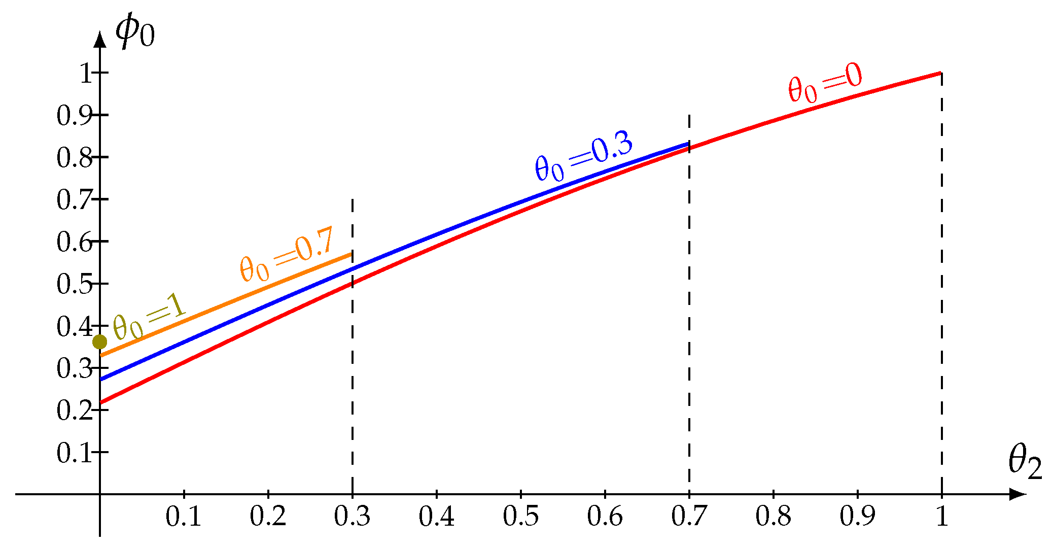
In Figure 1, we plot the probability that the system is empty (assuming the server is not under repair) against the parameter ${\theta }_2$. We display three curves corresponding to ${\theta }_0=0,0.3,1$. As expected, the probability ${\pi }_{0,0}$ increases with higher values of ${\theta }_2$ and ${\theta }_0$.

Figure 2 explains the behavior of the probability that the system is empty regardless of the server’s state against the parameter ${\theta }_2$ for various values of ${\theta }_0$. As expected, graphics 1 and 2 are very similar.

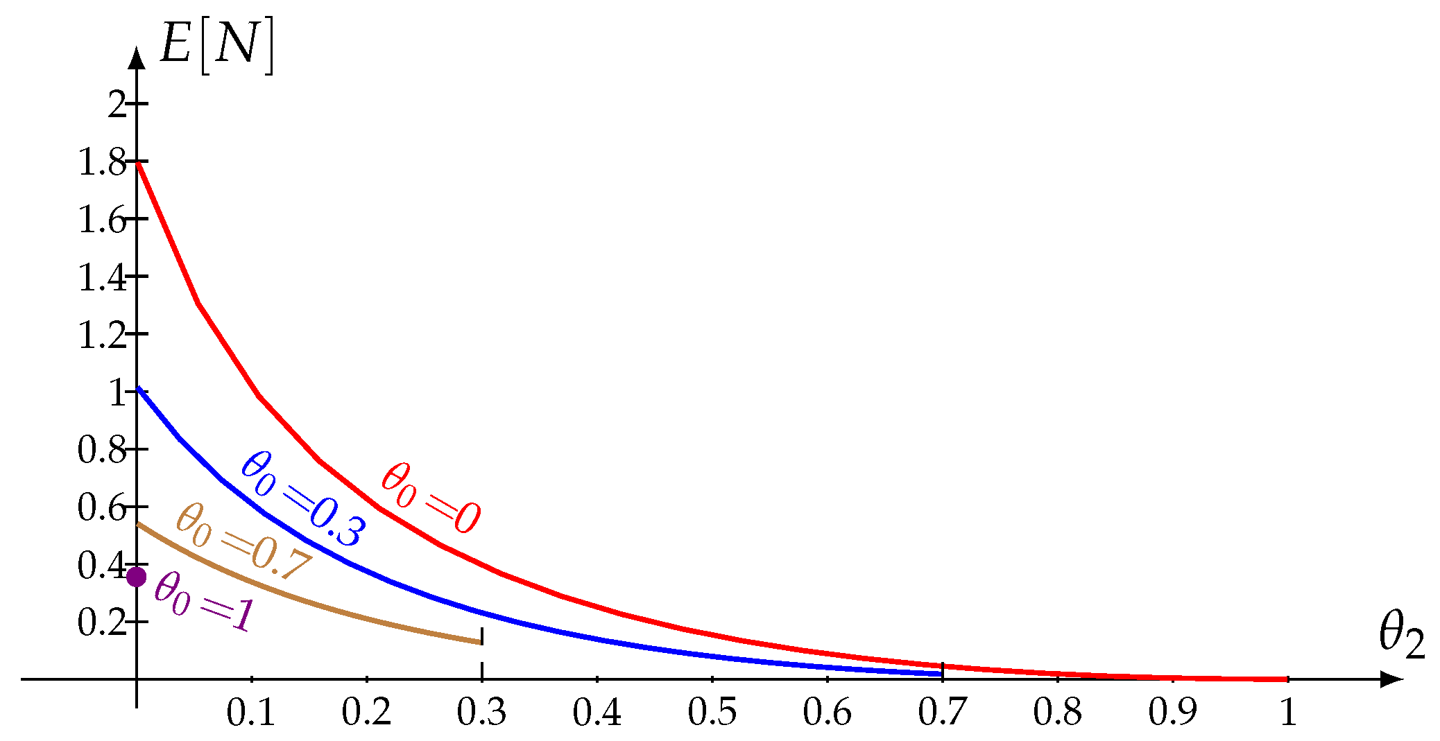
Figure 3 shows the mean number of retrial customers plotted against the parameter ${\theta }_2$ for various values of ${\theta }_0$. As intuition suggests, $E\left[N\right]$ decreases as the values of ${\theta }_2$ and ${\theta }_0$ increase.

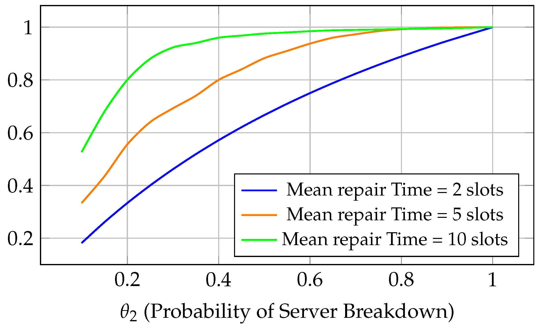
The graph in Figure 4 shows the probability of the server being under repair as a function of ${\theta }_2$ (the probability of a server breakdown). The analysis considers three different mean repair times: 2, 5, and 10 slots.

Observe that the three graphics are increasing functions of ${\theta }_2$ and of the mean repair time. As expected, a higher ${\theta }_2$ means more frequent breakdowns, leading to the server spending more time in the repair state. If we take into account the practical examples introduced in the first section, ${\theta }_2$ represents the probability of a system failure due to user overload or hardware issues, and reducing repair times (e.g., faster recovery procedures) significantly improves system availability. In production lines, where breakdowns disrupt operations, the graph suggests prioritizing shorter repair times (e.g., through better maintenance protocols) to minimize downtime.

The graphic in Figure 5 depicts the probability of the server being under repair as a function of the mean repair time ($E\left[R\right]$), for three values of ${\theta }_2$ (${\theta }_2=0.3,0.6,0.9$).

For all ${\theta }_2$ values, the probability that the server is in repair increases as $E\left[R\right]$ (mean repair time) increases. This makes intuitive sense: longer repair times increase the likelihood that the server will be under repair at any given moment.

Both call centers and manufacturing systems exhibit similar dynamics:

• The probability of being “under repair” increases with both higher breakdown probabilities (${\theta }_2$) and longer repair times ($E\left[R\right]$).
• Systems with frequent breakdowns (high ${\theta }_2$) benefit most from reducing $E\left[R\right]$, while systems with infrequent breakdowns may not see as significant of an improvement.
• These insights can guide resource allocation decisions, such as whether to focus on improving reliability (reducing ${\theta }_2$) or reducing repair times ($E\left[R\right]$).

10. Conclusions and Research Results

This study delves into a discrete-time retrial queuing system, where an arriving customer faces a choice: to follow a Last-Come-First-Served (LCFS) rule, pushing the current customer to the head of the orbit, or to join the orbit based on a First-Come-First-Served (FCFS) principle. The retrial intervals are broadly defined, allowing only the foremost customer in the orbit to access the server. Should a negative customer appear, they not only remove the active customer but also induce a server breakdown.

The development of generating functions for the number of customers, both in the orbit as well as in the whole system together with their average values, has been facilitated by a thorough investigation. In addition, the research looks into the steady-state stochastic decomposition property, providing bounds on the difference in variances between the limiting distributions of the queuing system considered and a similar benchmark system. The implications of the recursive algorithm transformed in Theorems 4 and 5 in determining the steady-state probabilities of customers in orbit and those within the system have emerged as one of the major features of this research. Further, the relationship of the continuous-time models with discrete-time models has also been explored.

We utilize the busy period of a system that could be considered an auxiliary one to evaluate the customer waiting time. This work has led to a major advance in retrial queue theory: finding the generating function for the steady-state distribution of customer orbit and system sojourn times. In the end, we can see figures showing how different parameters affect various performance metrics.

It is to be emphasized that the generating function technique is versatile and can be modified to solve retrial queues with a bursty access pattern and any type of distribution function. However, the complexity increases with the generality of the system, and alternative methods or approximations may be requisite in real implementations. This additional component appears to be interesting for future studies, especially those addressing the relationship between random access components and general or retrial service time distributions. Another interesting research area would be to study the continuous counterpart.