Generalizable Storm Surge Risk Modeling

Abstract

Storm surges present a severe risk to coastal communities and infrastructure, underscoring the critical importance of accurately estimating extreme events such as the 100-year return surge. These estimates are essential not only for effective hazard assessment but also for informing resilient coastal design. Inspired by principles of robust statistical modeling, this paper introduces a Bayesian hierarchical model integrated with Gaussian processes to account for spatial random effects. This approach enhances the precision of long return period storm surge estimates and enables the seamless generalization of predictions to nearby unmonitored coastal regions, much like the way advanced Bayesian frameworks are applied to high-dimensional neuroimaging or spatiotemporal data, bridging gaps between observations and uncharted territories.

1. Introduction

Coastal regions worldwide are highly vulnerable to flooding caused by abnormal sea level rises, often driven by intense storms such as tropical and extratropical cyclones. While non-tidal residuals may capture various anomalies beyond meteorological events, they generally serve as a reliable approximation for storm surges [1]. During extreme storm surge events, coastal defenses can be breached, resulting in extensive flooding that threatens infrastructure, assets, and coastal communities [2].

Bayesian hierarchical models (BHMs) offer a robust statistical alternative for coastal hazard assessment [3]. Unlike physics-based models, which rely on complex simulations, BHMs leverage observational data, such as tide gauge records, to estimate extreme return levels and interpolate them at ungauged locations. Historically, BHMs have been applied across diverse disciplines to analyze differences between related groups. For instance, ref. [4] (p. 387) employed a BHM to analyze temporal shifts in voting trends during U.S. Presidential elections, while [5] applied it to image label learning. More recent studies [6,7] have highlighted the utility of BHMs in coastal applications, demonstrating their effectiveness in interpolating unmonitored coastlines and significantly reducing uncertainty in extreme storm surge estimates.

In this study, we propose a BHM with a Generalized Extreme Value (GEV) likelihood [8], where the GEV parameters were modeled using linear models with spatially correlated random effects. Using a GEV generally allows for the modeling of maxima, e.g., extreme snowfalls [9], and optimal margin requirements for financial data [10]; in our case, this was the annual maximum storm surge at a given point along the coast of Florida. A Gaussian process (GP) [11] prior was applied to the random effects, allowing for the smooth interpolation of GEV parameters to nearby unmonitored locations.

GPs are widely used for modeling general functions, particularly in scenarios that require the incorporation of spatial and temporal correlations into geostatistical data. For instance, ref. [12] utilized GPs to model spatiotemporal correlations in COVID-19 deaths in Florida, while [13] applied GPs to analyze spatiotemporal patterns in deer mouse populations across the United States. Furthermore, ref. [14] extended the application of GPs to create spatially variable regressions for much denser datasets, addressing the computational challenges commonly encountered with standard GP methods. By applying GPs to model spatial correlations among the Generalized Extreme Value (GEV) parameters, our approach enables a robust estimation of long-term flood risks, even for unmonitored coastal regions.

This type of model has been used in existing work to model extrema, e.g., [3,7,15], typically by fixing one of the GEV parameters to be spatially invariant. In this work, we explored a different type of assumption by fixing the GEV distribution in the Fréchet regime [16] and setting the minimum to be 0.

Section 2 provides details of the proposed model. Section 3 presents a more detailed overview of the dataset and our findings, with validation and comparisons to other models in Section 4. Finally, Section 5 concludes with a discussion of the results and potential future research directions.

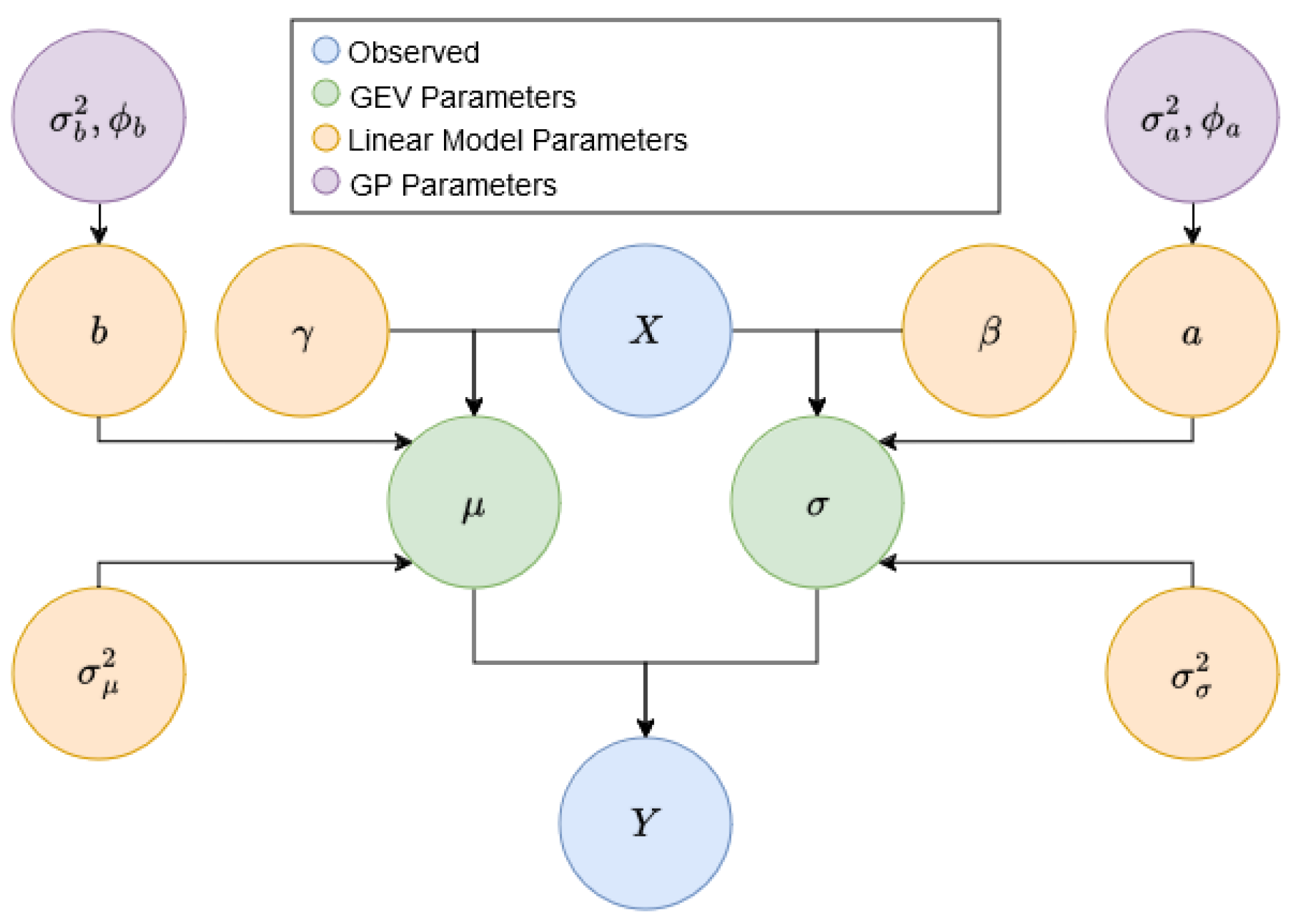
2. Methodology

Since the goal of our model was to create a system capable of estimating the GEV parameters at nearby unmonitored locations based on storm surge measurements at existing tide gauges, we created a hierarchical model of the GEV parameters using a regression on useful information such as the typical annual maximum rainfall at the location of interest, along with a spatial random effect GP, to model the GEV parameters. Figure 1 provides an overview of the model described in this section.

Figure 1. BHM overview. Y is the observed annual surge maxima; X is the covariates of interest.

To model the risk of storm surges in coastal areas over extended return periods, we made use of a GEV-based probability approach, following the methodology of [3]. The GEV was parameterized to model maxima as follows [8]:

$$\begin{array}{cc}\hfill p\left(y_{is}\right)& ={\displaystyle \frac{1}{{\sigma }_s}}{\left(1+{\xi }_s\left({\displaystyle \frac{y_{is}-{\mu }_s}{{\sigma }_s}}\right)\right)}^{-(1+{\displaystyle \frac{1}{{\xi }_s}})}exp\left(-{\left(1+{\xi }_s\left({\displaystyle \frac{y_{is}-{\mu }_s}{{\sigma }_s}}\right)\right)}^{-{\displaystyle \frac{1}{{\xi }_s}}}\right),\hfill \end{array}$$

where $s\in S$ represents a unique index for every location in the model, and $y_{is}$ represents the maximum surge observation in the ith year at location s, and ${\sigma }_s>0,{\xi }_s>0,y_{is}\in \left[{\mu }_s-{\displaystyle \frac{{\sigma }_s}{{\xi }_s}},\infty \right]$. The parameter ${\mu }_s$ is the location parameter of the GEV, representing the central tendency or horizontal position of the main mass of the distribution, while ${\sigma }_s$ is the scale parameter, indicating the spread or variability of the distribution. Throughout the paper, ${\mu }_s$ and ${\sigma }_s$ are referred to as $s\times 1$ vectors, representing the location and scale parameters for each location in the model. The general y is then a matrix, $n\times s$, where n is the maximum number of observations at any location, and s is the number of locations. This density is evaluated to be 1 when a given location does not have an observed maximum surge in a given year when evaluating the likelihood.

Since the application of interest was the annual maxima of storm surges, and these observations have a natural minimum at 0, we simplified the above by enforcing the condition that the shape parameter ${\xi }_s$ is constrained as follows:

$$\begin{array}{cc}\hfill {\xi }_s& ={\displaystyle \frac{{\sigma }_s}{{\mu }_s}}\hfill \end{array}$$

which enforces the minimum value of the support of the distribution to be 0. This assumption constitutes a significant difference from previous work in the area and allows for a full generalization to any possible value of future observations. We did not allow the model to fit any minimum above 0, as any positive value is a possible future annual surge maximum.

Next, we modeled ${\sigma }_s$ and ${\mu }_s$ at each location. As covariates like the typical annual minimum pressure, annual maximum wind speed, and annual maximum precipitation may be related to the annual storm surge maxima, we created a linear regression of these covariates and allowed for spatial random effects to capture any other differences not accounted for by the covariates. Thus, we modeled ${\sigma }_s$ and ${\mu }_s$ as noisy linear models with spatial random effects using a GP (e.g., [4,12]):

$$\begin{array}{ccc}\hfill ln\left({\sigma }_s\right)& ={\beta }^{\top }{X}_s+a_s+{ϵ}_{\sigma ,s},\hfill & \hfill {ϵ}_{\sigma ,s}\sim \mathrm{N}(0,{\sigma }_{\sigma }^2)\\ \hfill {\mu }_s& ={\gamma }^{\top }{X}_s+b_s+{ϵ}_{{\mu }_s,s},\hfill & \hfill {ϵ}_{{\mu }_s,s}\sim \mathrm{N}(0,{\sigma }_{{\mu }_s}^2),\end{array}$$

where $X_s$ denotes the sth row of a linear regression design matrix (including the constant for the intercept) for the covariates at the location indexed by s. In this analysis, we used the mean annual maxima for the precipitation and wind speed and the mean annual minimum for the sea level pressure at each location. $a_s$ and $b_s$ denote a spatially varying intercept with a Gaussian process prior over the vector of all $a_s$ or $b_s$, denoted as a or b:

$$\begin{array}{ccc}\hfill a& \sim \mathrm{N}(0,{\sigma }_a^2{K}_{{\varphi }_a}(S,S)),\hfill & \hfill {\sigma }_a^2\sim \mathrm{Gamma}(\alpha ,\theta )\\ \hfill b& \sim \mathrm{N}(0,{\sigma }_b^2{K}_{{\varphi }_b}(S,S)),\hfill & \hfill {\sigma }_b^2\sim \mathrm{Gamma}(\alpha ,\theta ),\end{array}$$

where $K_{\varphi }(S,S)$ represents the evaluation of a kernel function over the point-to-point distance matrix for all locations in S, and ${\sigma }_a^2$ and ${\sigma }_b^2$ are parameters that scale the GP appropriately to this dataset, deciding how much variance from location to location is due to the GP (higher values of these parameters) and how much is due to the error variance term. For this analysis, the squared exponential kernel was used:

$$\begin{array}{cc}\hfill K_{\varphi }(s,s^{\prime })& =e^{-\left(\mathrm{dist}{(s,s^{\prime })}^2\right)\varphi }\hfill \end{array}$$

$\varphi$ represents a scaling factor, related to how quickly the correlation between nearby locations decays to 0. High values of $\varphi$ indicate that only nearby areas contribute significantly to the prediction at a given location, while low values suggest broader spatial influence. Finally, the priors for the rest of the parameters are standard (conjugate if possible) priors:

$$\begin{array}{cc}\hfill \beta ,\gamma & \sim \mathrm{N}(0,{\sigma }_c^2{I}_p)\hfill \\ \hfill {\varphi }_a,{\varphi }_b& \sim \mathrm{Gamma}(\alpha ,\theta )\hfill \\ \hfill {\sigma }_{\sigma }^2,{\sigma }_{{\mu }_s}^2& \sim \mathrm{InvGamma}({\alpha }_{\sigma },{\beta }_{\sigma })\hfill \end{array}$$

where p denotes the number of covariates plus 1. All values left unspecified are hyperparameters. Summarizing the hierarchical model with the Bayes theorem, we have (denoting all parameters as $\psi$ for brevity)

$$\begin{array}{cc}\hfill p(\psi \mid y)& \propto \underset{\mathrm{GEV\; likelihood}}{\underbrace{p\left(y\right|{\mu }_s,{\sigma }_s)}}·\underset{\mathrm{Model\; for} {\sigma }_s}{\underbrace{p\left({\sigma }_s\right|\beta ,a,{\sigma }_{\sigma }^2)·p(\beta ,{\sigma }_{\sigma }^2)·p\left(a\right|{\varphi }_a,{\sigma }_a^2)·p({\varphi }_a,{\sigma }_a^2)}}·\underset{\mathrm{Model\; for} {\mu }_s}{\underbrace{p\left({\mu }_s\right|\gamma ,b,{\sigma }_{{\mu }_s}^2)·}}\hfill \end{array}$$

The priors for ${\mu }_s$ follow the same structure as the model for ${\sigma }_s$ described above, but are not shown as they do not fit on the line. The details of the posterior sampling procedure are provided in Algorithm 1.

Gibbs Sampling Algorithm

Let N represent the length of the simulation, let k be the number of locations with observations, and p be the number of covariates plus 1. For clarity, if a vector, z, with n elements is being initialized or updated, it is written as $z_{1:n}$; if it is instead a square matrix with $n\times n$ elements, it is written as $Z_{1:n}$.

Algorithm 1 Gibbs sampling algorithm

Initialize: ${\mu }_{1:k},{\sigma }_{1:k},{\beta }_{1:p},{\gamma }_{1:p},a_{1:k},b_{1:k},{\sigma }_{\sigma }^2,{\sigma }_{{\mu }_s}^2,{\sigma }_a^2,{\sigma }_b^2,{\varphi }_a,{\varphi }_b$ Set hyperparameters: ${\sigma }_c^2=10,{\alpha }_{\sigma }=0.001,{\beta }_{\sigma }=0.001,\alpha =1,\theta =100$ ${\mathsf{\Sigma }}_{1:p}\leftarrow {\sigma }_c^2{I}_p$ while  $i\le N$  do     $V_{1:p}\leftarrow {({\mathsf{\Sigma }}^{-1}+X^{\top }X{\displaystyle \frac{1}{{\sigma }_{\sigma }^2}})}^{-1}$                ▹ Gibbs update for $\beta$     $m_{1:p}\leftarrow V\left({\displaystyle \frac{1}{{\sigma }_{\sigma }^2}}{X}^{\top }(ln\left(\sigma \right)-a)\right)$     ${\beta }_{1:p}\leftarrow \mathrm{rMVNorm}(m,V)$     $V_{1:p}\leftarrow {({\mathsf{\Sigma }}^{-1}+X^{\top }X{\displaystyle \frac{1}{{\sigma }_{{\mu }_s}^2}})}^{-1}$                ▹ Gibbs update for $\gamma$     $m_{1:p}\leftarrow V\left({\displaystyle \frac{1}{{\sigma }_{{\mu }_s}^2}}{X}^{\top }({\mu }_s-b)\right)$     ${\gamma }_{1:p}\leftarrow \mathrm{rMVNorm}(m,V)$     ${ϵ}_{1:k}\leftarrow (ln\left(\sigma \right)-X\beta -a)$                 ▹ Gibbs update for ${\sigma }_{\sigma }^2$     ${\sigma }_{\sigma }^2\leftarrow \mathrm{rInvGamma}({\alpha }_{\sigma }+{\displaystyle \frac{k}{2}},{\beta }_{\sigma }+0.5·{ϵ}^{\top }ϵ)$     ${ϵ}_{1:k}\leftarrow ({\mu }_s-X\gamma -b)$                   ▹ Gibbs update for ${\sigma }_{{\mu }_s}^2$     ${\sigma }_{{\mu }_s}^2\leftarrow \mathrm{rInvGamma}({\alpha }_{\sigma }+{\displaystyle \frac{k}{2}},{\beta }_{\sigma }+0.5·{ϵ}^{\top }ϵ)$     $V_{1:k}\leftarrow {({\sigma }_a^2{K}_{{\varphi }_a}{(S,S)}^{-1}+{\displaystyle \frac{1}{{\sigma }_{\sigma }^2}}{I}_k)}^{-1}$              ▹ Gibbs update for a     $m_{1:k}\leftarrow V(ln\left(\sigma \right)-X\beta ){\displaystyle \frac{1}{{\sigma }_{\sigma }^2}}$     $a_{1:k}\leftarrow \mathrm{rMVNorm}(m,V)$     $V_{1:k}\leftarrow {({\sigma }_b^2{K}_{{\varphi }_b}{(S,S)}^{-1}+{\displaystyle \frac{1}{{\sigma }_{{\mu }_s}^2}}{I}_k)}^{-1}$              ▹ Gibbs update for b     $m_{1:k}\leftarrow V({\mu }_s-X\gamma ){\displaystyle \frac{1}{{\sigma }_{{\mu }_s}^2}}$     $b_{1:k}\leftarrow \mathrm{rMVNorm}(m,V)$     $z_{1:k}\leftarrow \mathrm{rNorm}(0,\mathrm{pmax}(0.02,0.25{\mu }_s))$             ▹ Metropolis–Hastings for ${\mu }_s$     $l{u}_{1:k}\leftarrow ln\left(\mathrm{rUnif}(0,1)\right)$     for $s\in [1,\dots ,k]$ do         ${\mu }_s^{\prime }\leftarrow {\mu }_s+z_s$         ${\xi }_s={\displaystyle \frac{{\sigma }_s}{{\mu }_s}}$         ${\xi }_s^{\prime }={\displaystyle \frac{{\sigma }_s}{{\mu }_s^{\prime }}}$         $l\leftarrow \mathrm{sum}\left(\mathrm{dGev}\right(y_s,{\mu }_s,{\sigma }_s,{\xi }_s,\log =\mathrm{T}\left)\right)+\mathrm{dNorm}({\mu }_s,{\gamma }^{\top }{X}_s+b,{\sigma }_{\sigma },\log =\mathrm{T})$         $l^{\prime }\leftarrow \mathrm{sum}\left(\mathrm{dGev}\right(y_s,{\mu }_s^{\prime },{\sigma }_s,{\xi }_s^{\prime },\log =\mathrm{T}\left)\right)+\mathrm{dNorm}({\mu }_s^{\prime },{\gamma }^{\top }{X}_s+b,{\sigma }_{\sigma },\log =\mathrm{T})$         if $l^{\prime }-l>l{u}_s$ then ${\mu }_s={\mu }_s^{\prime }$         end if     end for     $z_{1:k}\leftarrow \mathrm{rNorm}(0,\mathrm{pmax}(0.001,0.25\sigma ))$             ▹ Metropolis–Hastings for $\sigma$     $l{u}_{1:k}\leftarrow ln\left(\mathrm{rUnif}(0,1)\right)$     for $s\in [1,\dots ,k]$ do         ${\sigma }_s^{\prime }\leftarrow {\sigma }_s+z_s$         ${\xi }_s={\displaystyle \frac{{\sigma }_s}{{\mu }_s}}$         ${\xi }_s^{\prime }={\displaystyle \frac{{\sigma }_s^{\prime }}{{\mu }_s}}$         $l\leftarrow \mathrm{sum}\left(\mathrm{dGev}\right(y_s,{\mu }_s,{\sigma }_s,{\xi }_s,\log =\mathrm{T}\left)\right)+\mathrm{dNorm}(ln\left({\sigma }_s\right),{\beta }^{\top }{X}_s+a,{\sigma }_{\sigma },\log =\mathrm{T})$         $l^{\prime }\leftarrow \mathrm{sum}\left(\mathrm{dGev}\right(y_s,{\mu }_s,{\sigma }_s^{\prime },{\xi }_s^{\prime },\log =\mathrm{T}\left)\right)+\mathrm{dNorm}(ln\left({\sigma }_s^{\prime }\right),{\beta }^{\top }{X}_s+a,{\sigma }_{\sigma },\log =\mathrm{T})$         if $l^{\prime }-l>l{u}_s$ then ${\sigma }_s={\sigma }_s^{\prime }$         end if     end for     $z\leftarrow \mathrm{rNorm}(0,\mathrm{pmax}(2,0.25{\varphi }_a))$                ▹ Metropolis–Hastings for ${\varphi }_a$     $lu\leftarrow ln\left(\mathrm{rUnif}\right(0,1\left)\right)$     ${\varphi }_a^{\prime }\leftarrow {\varphi }_a+z$     $l\leftarrow \mathrm{dMVNorm}(a,{\sigma }_a^2{K}_{{\varphi }_a}(S,S),\log =\mathrm{T})+\mathrm{dGamma}({\varphi }_a,\alpha ,\theta ,\log =\mathrm{T})$     $l^{\prime }\leftarrow \mathrm{dMVNorm}(a,{\sigma }_a^2{K}_{{\varphi }_a^{\prime }}(S,S),\log =\mathrm{T})+\mathrm{dGamma}({\varphi }_a^{\prime },\alpha ,\theta ,\log =\mathrm{T})$     if $l^{\prime }-l>lu$ then ${\varphi }_a={\varphi }_a^{\prime }$     end if     MH for ${\varphi }_b$, same as above but with b instead of a        ▹ Metropolis–Hastings for ${\varphi }_b$     $z\leftarrow \mathrm{rNorm}(0,\mathrm{pmax}(0.001,0.25{\sigma }_a^2))$               ▹ Metropolis–Hastings for ${\sigma }_a^2$     $lu\leftarrow ln\left(\mathrm{rUnif}\right(0,1\left)\right)$     ${\sigma }_a^{2^{\prime }}\leftarrow {\sigma }_a^2+z$     $l\leftarrow \mathrm{dMVNorm}(a,{\sigma }_a^2{K}_{{\varphi }_a}(S,S),\log =\mathrm{T})+\mathrm{dGamma}({\sigma }_a^2,\alpha ,\theta ,\log =\mathrm{T})$     $l^{\prime }\leftarrow \mathrm{dMVNorm}(a,{\sigma }_a^{2^{\prime }}{K}_{{\varphi }_a}(S,S),\log =\mathrm{T})+\mathrm{dGamma}({\sigma }_a^{2^{\prime }},\alpha ,\theta ,\log =\mathrm{T})$     if $l^{\prime }-l>lu$ then ${\sigma }_a^2={\sigma }_a^{2^{\prime }}$     end if     MH for ${\sigma }_b^2$, same as above but with b instead of a        ▹ Metropolis–Hastings for ${\sigma }_b^2$ end while

The sequential Gibbs algorithm to sample all parameters (and not predict at new locations) was run at a speed of 100 iterations in 20 s on a i7-13700k processor. A total of 200,000 iterations were run to ensure convergence, requiring approximately 12 h of computation time. This algorithm was implemented in Python using the Numpy [17] and Scipy [18]. Gaussian process-based predictions at each point can be generated subsequently on a GPU for increased efficiency.

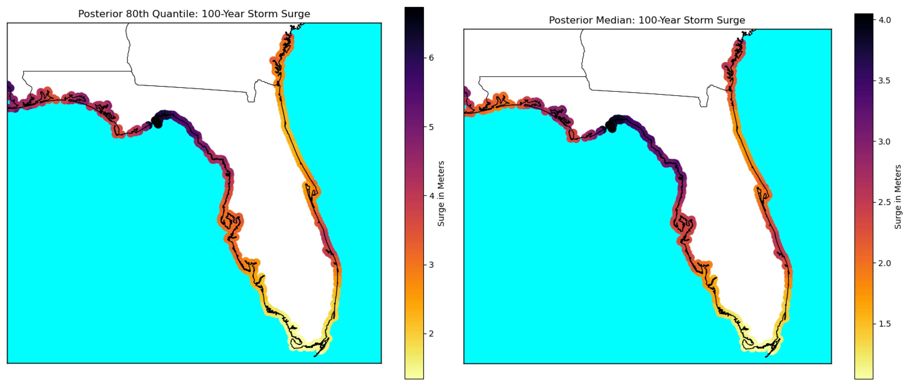
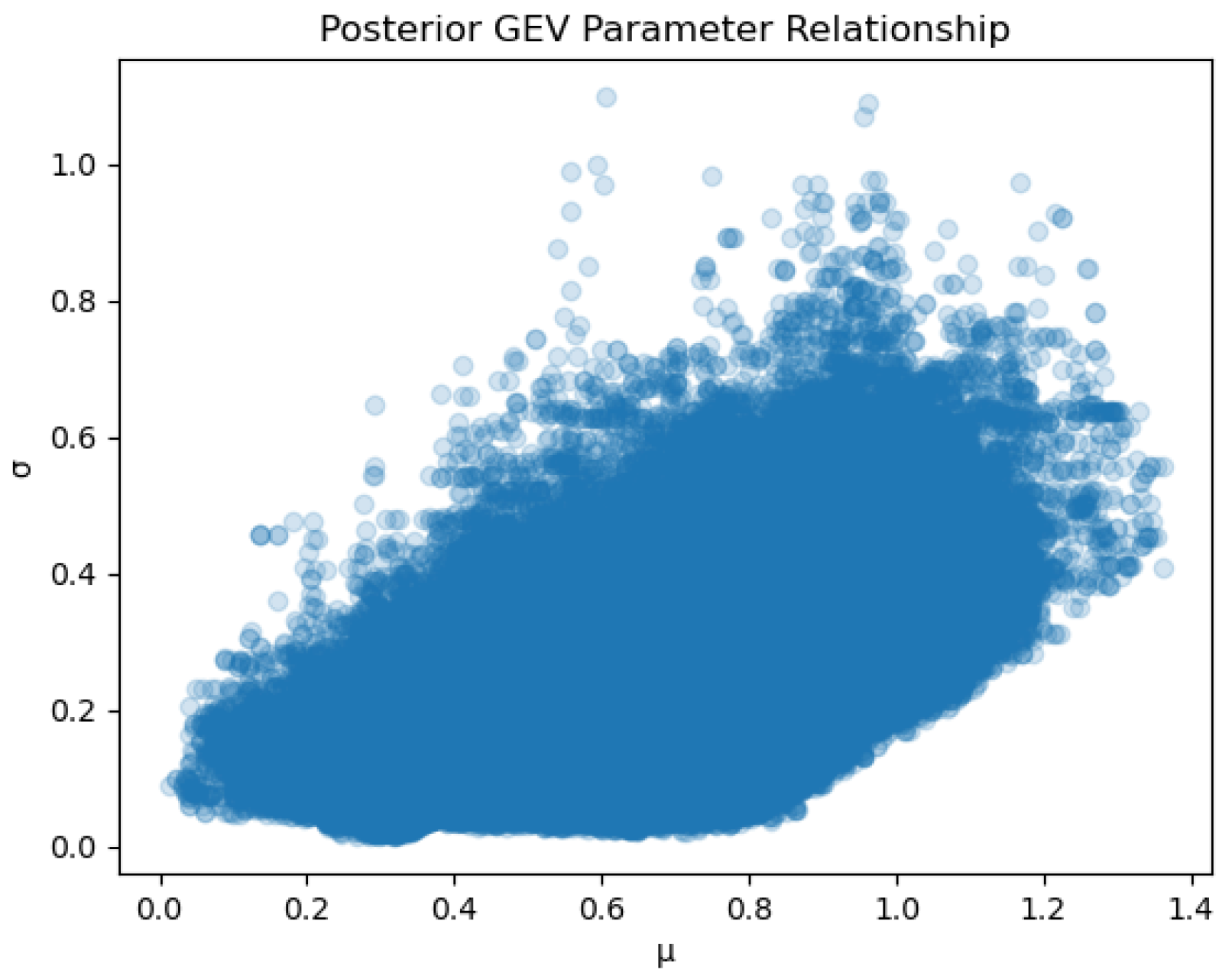
3. Application Details and Results

We applied the model described in Section 2 to tidal gauge data from the National Oceanic and Atmospheric Administration (NOAA) Tides and Currents [19] for the state of Florida, covering the period from 1979 to 2019. The annual maximum storm surge each year was used to train GEV parameters at each tide gauge location. Additionally, we utilized the ERA5 dataset from the European Centre for Medium-Range Weather Forecasts (ECMWF) [20], which provides hourly atmospheric covariate values for each location. Specifically, we used the mean annual maximum wind speed, minimum sea level pressure, and maximum precipitation in our model of the location (${\mu }_s$) and scale ($\sigma$) parameters for the GEV distribution at each location within the dataset. These predictors were first standardized before fitting to account for the large differences in scale.

Based on the resulting linear models for ${\mu }_s$ and $\sigma$, we then predicted the GEV parameters at each location along the Florida coastline with each model seen in the Gibbs samples and constructed credible intervals for the 100-year return period storm surge, among other values of interest. The upper bound of a 60% (quantile-based) credible interval for the 100-year storm surge is shown in Figure 2. We used 60% credible intervals for this image since some locations only had 1–3 years with enough data to obtain an annual maximum storm surge, and thus the posterior distributions of their parameters were highly variable, resulting in some unrealistic results in the upper and lower 10–15% of the results. Based on the results of this model, the area most at risk for large storm surges in Florida is the area around Apalachee Bay, where we estimated an upper bound for 100-year storm surges at around 6 m.

Figure 2. (Left): The 80th percentile upper bound for 100-year storm surges based on data from 1979 to 2019. (Right): Posterior median for the same.

Examining the coefficients for ${\mu }_s$ in Table 1, we observed that the sea level pressure was the only significant predictor. When rescaled to the original data units, this indicates that a $146.7$ pascal decrease in the mean annual minimum sea level pressure at a location is associated with an expected increase of $0.038$ to $0.199$ m in the location parameter of the GEV distribution for the annual maximum surge at that location. However, this does not necessarily mean that the storm surge at that location will increase by the same amount, as the correlated GEV scale parameter may partially offset this effect, as shown in Figure 3.

Table 1. The 95% credible intervals for the model coefficients ($\gamma$) for ${\mu }_s$.

Regression Coefficient	95% C.I.
Intercept	$[0.178,0.773]$
Sea Level Pressure	$[-0.199,-0.038]$
Wind	$[-0.060,0.016]$
Precipitation	$[-0.066,0.030]$

Figure 3. Relationship between GEV ${\mu }_s$ and $\sigma$ parameters in posterior samples.

The lack of significance for wind data might be due to their inability to account for the direction of the strongest winds or the broader wind field as a whole, potentially reducing their correlation with typical storm surge estimates. Similarly, the precipitation covariate could benefit from being expanded to consider conditions in nearby areas, rather than relying solely on the typical annual maximum hourly precipitation at a given location.

Finally, based on the 95% credible interval for the GP parameters for the spatially varying intercept for ${\mu }_s$ in Table 2, nearly all sampled models estimated the correlation between intercepts at locations less than 50 miles apart to be 0.2 or greater, with estimates for where the correlation decays to 0.2 varying from between about 50 to about 300 miles in distance. The error variance for ${\mu }_s$ was estimated to lie between 0.001 and 0.009 with 95% credibility. Additionally, we estimated that the spatial Gaussian process accounted for 1.027 to 141 times more variance in ${\mu }_s$ between locations than the error term, also with 95% credibility.

Table 2. The 95% credible intervals for the GP parameters for ${\mu }_s$.

Parameter	95% C.I.
$\varphi$	$[3.03,133.7]$
${\sigma }_b^2$	$[0.0061,0.34]$

4. Validation

To validate our results, we conducted a simulation using data generated according to the assumptions of our model, verifying that the credible intervals produced by the model can recover the true parameters. Specifically, we generated 50 yearly maxima at 20 locations, incorporating three covariates and an intercept, as in the main analysis, and applied the model to the resulting dataset. As shown in Table 3, the model and the Gibbs sampling method demonstrated the ability to broadly recover the true parameters.

Table 3. (Top): Recovery of simulated parameters. Bolded rows are parameters that were recovered. (Bottom): Comparison of 95% CI for 100-year flood estimates based on MLE and our model. Simulated Location 3 violates asymptotic normality assumption for MLE.

Parameter	True Value	95% CI/Coverage Proportion
${\mathit{\mu }}_{\mathit{s}}$	Vector	90%
${\mathit{\sigma }}_{\mathit{s}}$	Vector	95%
$\mathit{\beta }$	Vector	100%
$\mathit{\gamma }$	Vector	100%
$\mathit{a}$	Vector	95%
b	Vector	80%
${\sigma }_{{\mu }_s}^2$	0.2	[0.53, 2.5]
${\mathit{\sigma }}_{\mathit{\sigma }}^{\mathbf{2}}$	0.2	[0.12, 1.05]
${\mathit{\sigma }}_{\mathit{a}}^{\mathbf{2}}$	0.5	[0.04, 1.56]
${\mathit{\sigma }}_{\mathit{b}}^{\mathbf{2}}$	0.6	[0.012, 1.86]
${\mathit{\varphi }}_{\mathit{a}}$	60	[10.7, 230.8]
${\mathit{\varphi }}_{\mathit{b}}$	90	[5.23, 200.6]
Location	MLE	Our BHM	True
1, Sim	[7.01, 9.05]	[7.36, 9.76]	8.5
3, Sim	[−300,000, 618,000]	[12,000, 2,030,000]	166,000
10, Sim	[24.4, 144]	[50.6, 214]	88
Naples	[1.2, 2.88]	[1.41, 2.67]
Clearwater	[1.15, 2.72]	[1.60, 3.33]
Eastpoint	[1.24, 4.01]	[1.15, 2.73]

In other simulation runs, we observed that the variance parameters were only recovered properly when the kernel variance (${\sigma }_a^2$, ${\sigma }_b^2$) was at around the same scale as the noise variance (${\sigma }_{{\mu }_s}^2$, ${\sigma }_{\sigma }^2$) and that the noise variance parameters were sometimes overestimated, as we also saw in this simulation run for ${\sigma }_{{\mu }_s}^2$.

To further validate our results, we compared the results of using the maximum likelihood estimators (MLEs) for ${\mu }_s$ and $\sigma$ at each individual location to our results for a few locations in the simulated dataset and the actual storm surge data. We used the delta method to estimate the variance in the MLE estimate for the 100-year floods. On the simulated dataset, predictions from our model and predictions from the MLE estimates were fairly comparable, except for the location where the simulated dataset had $\sigma >{\mu }_s$, under which conditions the lower bounds for the MLE estimates for 100-year return period floods using the delta method were negative due to the violation of the asymptotic normality assumption.

On the actual dataset, our model also performed similarly to the MLE estimates, though often with less variance in the predicted 100-year flood when there were not many yearly maxima to go off of at a given location, as is the case with Eastpoint in Table 3.

5. Discussion

BHMs provide a robust alternative to standard extreme value techniques, particularly for spatially distributed data. Consistent with the results of [3], our analysis demonstrates that BHMs with GPs effectively reduced the variability of 100-year storm surge estimates at sparsely monitored locations, while maintaining performance comparable to that of standard MLE methods when this additional capability was not required. Furthermore, the use of GPs enabled the seamless generalization of estimates to unmonitored locations, enhancing their practical utility for coastal hazard assessment.

Among our covariates, only the coefficient for the mean annual minimum sea level pressure was significant, indicating that low pressures are more consistently linked to storm surges than wind speeds or precipitation amounts. In the future, methods to use the full wind field over a location of interest from ERA5 [20] to predict storm surges at a location, rather than just the wind speed at the nearest location, should be considered.

In our simulation study, we observed that the Gaussian processes (GPs) in our model could effectively distinguish between noise variance and kernel variance only when these parameters were of similar scales (within roughly one order of magnitude). Further exploration of the underlying causes of this limitation, along with the development of advanced modeling techniques to overcome it, represents a critical avenue for future research.

References

- Wahl, T.; Jain, S.; Bender, J.; Meyers, S.D.; Luther, M.E. Increasing risk of compound flooding from storm surge and rainfall for major US cities. Nat. Clim. Chang. 2015, 5, 1093–1097. [Google Scholar] [CrossRef]
- Wahl, T.; Haigh, I.D.; Nicholls, R.J.; Arns, A.; Dangendorf, S.; Hinkel, J.; Slangen, A.B.A. Understanding extreme sea levels for broad-scale coastal impact and adaptation analysis. Nat. Commun. 2017, 8, 16075. [Google Scholar] [CrossRef] [PubMed]
- Boumis, G.; Moftakhari, H.R.; Moradkhani, H. Storm surge hazard estimation along the US Gulf Coast: A Bayesian hierarchical approach. Coast. Eng. 2023, 185, 104371. [Google Scholar] [CrossRef]
- Gelman, A.; Carlin, J.B.; Stern, H.S.; Dunson, D.B.; Vehtari, A.; Rubin, D.B. Bayesian Data Analysis, 3rd ed.; Texts in statistical science series; CRC Press, Taylor and Francis Group: Boca Raton, FL, USA; London, UK; New York, NY, USA, 2014. [Google Scholar]
- Fei-Fei, L.; Perona, P. A Bayesian hierarchical model for learning natural scene categories. In Proceedings of the 2005 IEEE Computer Society Conference on Computer Vision and Pattern Recognition (CVPR’05), San Diego, CA, USA, 20–26 June 2005; Volume 2, pp. 524–531, ISSN: 1063-6919. [Google Scholar] [CrossRef]
- Beck, N.; Genest, C.; Jalbert, J.; Mailhot, M. Predicting extreme surges from sparse data using a copula-based hierarchical Bayesian spatial model. Environmetrics 2020, 31, e2616. [Google Scholar] [CrossRef]
- Calafat, F.M.; Marcos, M. Probabilistic reanalysis of storm surge extremes in Europe. Proc. Natl. Acad. Sci. USA 2020, 117, 1877–1883. [Google Scholar] [CrossRef] [PubMed]
- Kotz, S.; Nadarajah, S. Extreme Value Distributions: Theory and Applications; World Scientific: Singapore, 2000. [Google Scholar]
- Blanchet, J.; Marty, C.; Lehning, M. Extreme value statistics of snowfall in the Swiss Alpine region. Water Resour. Res. 2009, 45. [Google Scholar] [CrossRef]
- Cotter, J. Margin exceedences for European stock index futures using extreme value theory. J. Bank. Financ. 2001, 25, 1475–1502. [Google Scholar] [CrossRef]
- Rasmussen, C.E.; Williams, C.K.I. Gaussian Processes for Machine Learning, 3rd ed.; Adaptive Computation and Machine Learning; MIT Press: Cambridge, MA, USA, 2008. [Google Scholar]
- He, Q.; Huang, H.H. A framework of zero-inflated Bayesian negative binomial regression models for spatiotemporal data. J. Stat. Plan. Inference 2024, 229, 106098. [Google Scholar] [CrossRef]
- Huang, H.H.; He, Q. Statistical modeling of Peromyscus maniculatus (deer mouse) amounts per trap with spatiotemporal data. Jpn. J. Stat. Data Sci. 2023, 6, 847–860. [Google Scholar] [CrossRef]
- Banerjee, S.; Gelfand, A.E.; Finley, A.O.; Sang, H. Gaussian Predictive Process Models for Large Spatial Data Sets. J. R. Stat. Soc. Ser. B Stat. Methodol. 2008, 70, 825–848. [Google Scholar] [CrossRef] [PubMed]
- Ghosh, S.; Mallick, B.K. A hierarchical Bayesian spatio-temporal model for extreme precipitation events. Environmetrics 2011, 22, 192–204. [Google Scholar] [CrossRef]
- Huang, H.H.; Yu, F.; Li, K.; Zhang, T. Frechet Sufficient Dimension Reduction for Metric Space-Valued Data via Distance Covariance. arXiv 2024, arXiv:2412.13122. [Google Scholar]
- Harris, C.R.; Millman, K.J.; van der Walt, S.J.; Gommers, R.; Virtanen, P.; Cournapeau, D.; Wieser, E.; Taylor, J.; Berg, S.; Smith, N.J.; et al. Array programming with NumPy. Nature 2020, 585, 357–362. [Google Scholar] [CrossRef] [PubMed]
- Virtanen, P.; Gommers, R.; Oliphant, T.E.; Haberland, M.; Reddy, T.; Cournapeau, D.; Burovski, E.; Peterson, P.; Weckesser, W.; Bright, J.; et al. SciPy 1.0: Fundamental algorithms for scientific computing in Python. Nat. Methods 2020, 17, 261–272. [Google Scholar] [CrossRef] [PubMed]
- Center for Operational Oceanographic Products and Services. Tides/Water Levels. 2024. Available online: https://tidesandcurrents.noaa.gov/products.html (accessed on 7 December 2024).
- Hersbach, H.; Bell, B.; Berrisford, P.; Hirahara, S.; Horányi, A.; Muñoz-Sabater, J.; Nicolas, J.; Peubey, C.; Radu, R.; Schepers, D.; et al. The ERA5 global reanalysis. Q. J. R. Meteorol. Soc. 2020, 146, 1999–2049. [Google Scholar] [CrossRef]