Population-Based Search Algorithms for Biopharmaceutical Manufacturing Scheduling Problem with Heterogeneous Parallel Mixed Flowshops

Abstract

In this paper, we address biopharmaceutical manufacturing scheduling problems with heterogeneous parallel mixed flowshops. The mixed flowshop consists of three stages, one batch process and two continuous processes. The objective function is to minimize the total tardiness. We formulated a mixed-integer linear programming model for the problem to obtain optimal solutions to small-size problems. We present a genetic algorithm and particle swarm optimization, which are used to find efficient solutions for large-size problems. We show that the particle swarm optimization outperforms the genetic algorithm in large-size problems. We conduct a sensitivity analysis to obtain managerial insights using the particle swarm optimization algorithm.

1. Introduction

Biopharmaceuticals are drugs developed using cells, tissues, hormones, etc., derived from humans or other organisms. Global demand for biopharmaceuticals is increasing due to factors such as the aging population, the increasing incidence of chronic diseases, and the increasing importance of personalized medicine. Accordingly, the biopharmaceutical market is growing steadily [1]. Figure 1 shows the biopharmaceutical process. Biopharmaceuticals are made through three processes: (1) the upstream process (USP) and (2) the downstream process (DSP) of the drug substance (DS) and (3) the drug product (DP). The DS process treats active ingredients. The DS process is divided into an upstream process (USP) and a downstream process (DSP). The USP corresponds to the cell culture stage and the DSP corresponds to the purification and polishing stage [2]. The DP produces the finished drugs based on DS [3].

The biopharmaceutical manufacturing process has unique characteristics unlike other manufacturing processes. First, consistent cleaning and sterilization are required to avoid cross-contamination in biopharmaceuticals. So, a setup time is generated depending on the product-type sequence. Second, a flowshop or jobshop environment rather than a single process is common. This is because biopharmaceuticals are generally made using several processes. Also, multiple flowshops or jobshops often exist within one factory to improve productivity. Additionally, the specifications, such as processing speed and capacity, of each flowshop or jobshop are generally different. Finally, mixed flowshop environments that mix batch and continuous manufacturing are common. Figure 2 shows schematics of batch and continuous manufacturing, respectively. As shown in Figure 2a, in batch manufacturing, all raw materials are input before the chemical reaction/refining operations, and the product is discharged after all of these processes are completed. Meanwhile, as shown in Figure 2b, the processes of raw material input, chemical reaction/refining, and product discharge occur continuously in continuous manufacturing. The biopharmaceutical process is shifting towards continuous manufacturing to meet the increasing demand for biopharmaceutical products [4]. However, it is challenging to produce biopharmaceuticals by only using continuous manufacturing because cleaning and sterilization are difficult in continuous manufacturing. Therefore, mixed flowshop environments are common in biopharmaceutical manufacturing. The improvement in productivity when changing the batch process to a mixed process is shown in Figure 3. Figure 3a,b show an example of a Gantt chart for batch manufacturing and mixed flowshop environments, respectively, supposing that three products are to be processed and there are three processes for batch and mixed flowshop manufacturing. As shown in Figure 3a, in batch manufacturing, all materials are charged before the process begins and discharged at the end of the process [5]. Since intermediates are not transferred directly to the next manufacturing process, a bottleneck occurs and the efficiency of biopharmaceutical production decreases [6]. Unlike batch manufacturing, as shown in Figure 3b, in two adjacent continuous processes of mixed flowshop manufacturing, materials are continuously charged and discharged during the process [5]. Thus, unlike batch manufacturing, bottlenecks do not occur in mixed flowshop. Eliminating bottlenecks can potentially increase product quantity and responsiveness, and improve overall drug quality [7].

The contributions of this study are fourfold. First, to the best of our knowledge, we address the biopharmaceutical manufacturing scheduling problem with heterogeneous parallel mixed flowshops (BPMSP-HPMFSs) for the first time. Second, we develop a mixed-integer linear programming (MILP) model for the problem to find an optimal solution for small-sized problems. As mentioned in the explanation of Figure 3, continuous manufacturing has structural differences from traditional batch manufacturing. The contribution of the mathematical model is that these differences are reflected in the MILP model. Third, we present a genetic algorithm (GA) and particle swarm optimization (PSO) to find an efficient solution for large-sized problems. Finally, we perform a sensitivity analysis to obtain managerial insights.

The remainder of the paper is organized as follows. In Section 2, we review and categorize relevant studies. In Section 3, we describe the presented problem and formulate the MILP model. In Section 4, we present the GA and PSO with the same solution structure. In Section 5, we verify and evaluate the performance of the proposed GA and PSO. In Section 6, we perform the sensitivity analysis to obtain managerial insights.

2. Related Work

In this section, we review and categorize the studies on pharmaceutical manufacturing scheduling. Kopanos et al. [8] addressed an iterative two-stage MIP-based solution to solve real-world scheduling problems in a multi-stage multi-product batch plant. The objective is to minimize the makespan and total weighted lateness. Kim et al. [9] addressed a new mathematical model that combines MILP and heuristic techniques that minimize the makespan in actual pharmaceutical intermediates manufacturing (PIM) factories. Raaymakers and Hoogeveen [10] addressed scheduling problems in multi-purpose batch processing industries. The scheduling problems are characterized as multiprocessor no-wait jobshop with overlapping operations. A simulated algorithm (SA) was developed to minimize the makespan. Kabra et al. [11] developed a continuous-time model for multi-period, multi-stage, and multi-product scheduling in the biopharmaceutical industry. A state–task network (STN)-based MILP was developed by extending the model developed by Shaik and Floudas [12]. Castro et al. [13] addressed a mathematical formulation for scheduling multi-purpose plants involving batch or continuous processes based on resource–-task network (RTN) representations. Vieira et al. [14] developed an MILP formulation extending the unified continuous-time RTN representation presented by Castro et al. [13]. The model reflected two of the characteristics of bioprocesses scheduling, the traceability of different productions and the shelf-life storage limitations. Costa [15] addressed the real-life batch scheduling problem of parallel machines in constrained environments. A hybrid genetic algorithm (HGA) with two-step encoding was proposed to increase the production speed and obtain a quick solution that could satisfy the company’s requirements. Jankauskas et al. [16] developed a GA to quickly solve the discrete-time problem of capacity planning and scheduling in the pharmaceutical industry. Awad et al. [17] introduced a constraint programming (CP) model to solve a large-scale scheduling problem in a batch pharmaceutical manufacturing plant. Aguirre et al. [18] developed a method combining RH and II algorithms and full-space MILP models to solve medium-scale planning and scheduling problems in multi-product, multi-stage continuous plants. Vieira et al. [19] present an optimal planning method for the biopharmaceutical continuous manufacturing process with an MILP model based on the RTN continuous single-time grid formulation. Vieira et al. [20] present a hybrid flowshop scheduling problem that mixes batch and continuous manufacturing in pharmaceutical manufacturing for the first time. They developed a new MILP model based on an RTN continuous-time single-grid formulation. In addition to pharmaceutical scheduling, there are studies on scheduling in a multi-flowshop machine environment. The term “parallel flowshops” first appeared in work by Sevastyanov et al. [21], which was previously referred to as “parallel two-stage systems”, a similar concept but with a different name [22]. It is also called “distributed flowshops”. Dolgui et al. [23] studied a distributed two-machine flowshop scheduling problem.

Table 1. Related studies on BPMSP-HPMFSs.

Article	Manufacturing Environment		Production Method			Machine Velocity		Setup			Problem Size
	(a)	(b)	(c)	(d)	(e)	(f)	(g)	(h)	(i)	(j)	(k)	(l)
Kopanos et al. [8]	✓		✓			✓		✓	✓			✓
Kim et al. [9]		✓	✓			✓		✓		✓		✓
Raaymakers and Hoogeveen [10]		✓	✓			✓						✓
Kabra et al. [11]	✓		✓				✓	✓	✓		✓
Castro et al. [13]			✓	✓		✓						✓
Vieira, et al. [14]	✓		✓				✓				✓
Costa [15]	✓		✓			✓		✓	✓			✓
Jankauskas et al. [16]	✓		✓			✓			✓			✓
Awad et al. [17]	✓		✓					✓			✓
Aguirre et al. [18]	✓			✓		✓		✓
Vieira et al. [19]	✓			✓		✓		✓
Vieira et al. [20]	✓				✓	✓		✓			✓
Our study	✓				✓		✓	✓				✓

(a): flowshop; (b): jobshop; (c): batch; (d): continuous; (e): mixed; (f): homogeneous; (g): heterogeneous; (h): sequence-dependent; (i): sequence-independent; (j): unit-dependent; (k): small; (l): large.

shows studies related to BPMSP-HPMFS, classified according to the manufacturing environment, production method, machine velocity, setup, problem size, and solution method. As shown in Table 1, we present the BPMSP-HPMFSs for the first time. Although Vieira et al. [20] addressed the flowshop scheduling problem with hybrid production that mixes batch and continuous manufacturing, it has the limitation of not providing a solution to the large size of the problem. Additionally, they assumed a homogeneous machine environment where the machines have the same processing velocity. In contrast, we assume a heterogeneous machine environment where the machine’s processing speed is different.

3. Problem Description

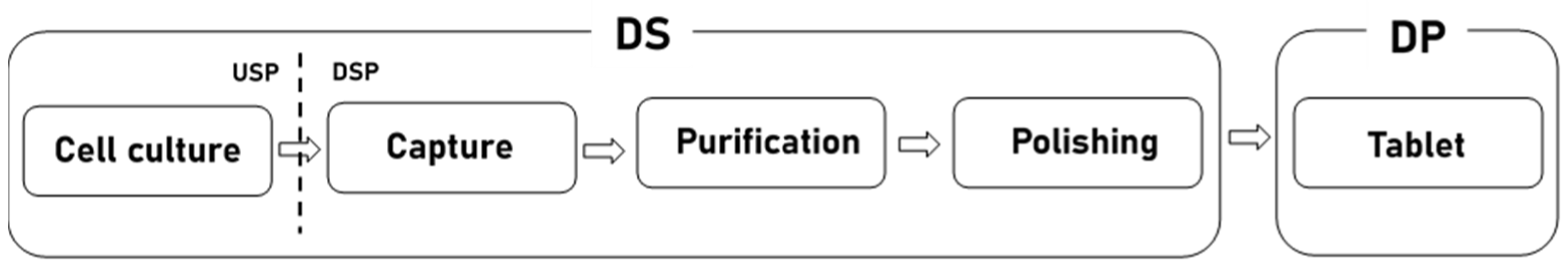
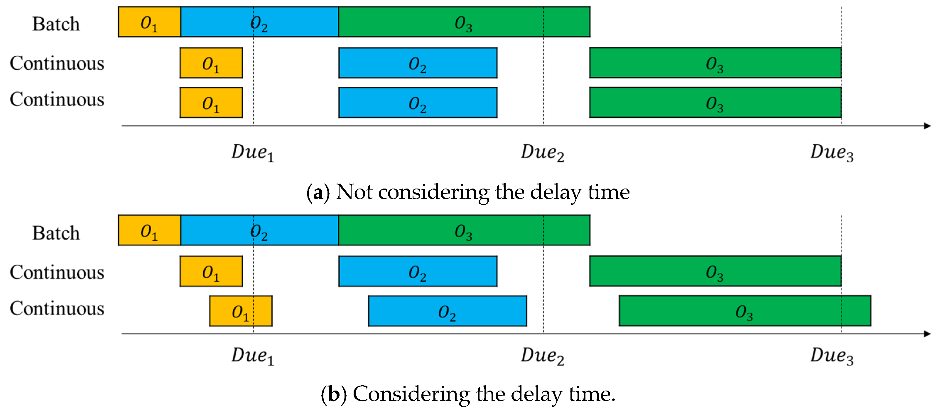
3.1. Biopharmaceutical Manufacturing Scheduling Problem with Heterogeneous Parallel Mixed Flowshops (BPMSP-HPMFSs)

In this section, we address the BPMSP-HPMFSs. The objective is to minimize the total tardiness by determining two decisions: assigning the orders to the flowshops and sequencing the assigned orders within each flowshop. The characteristics and assumptions of the presented problem are as follows:

(1)

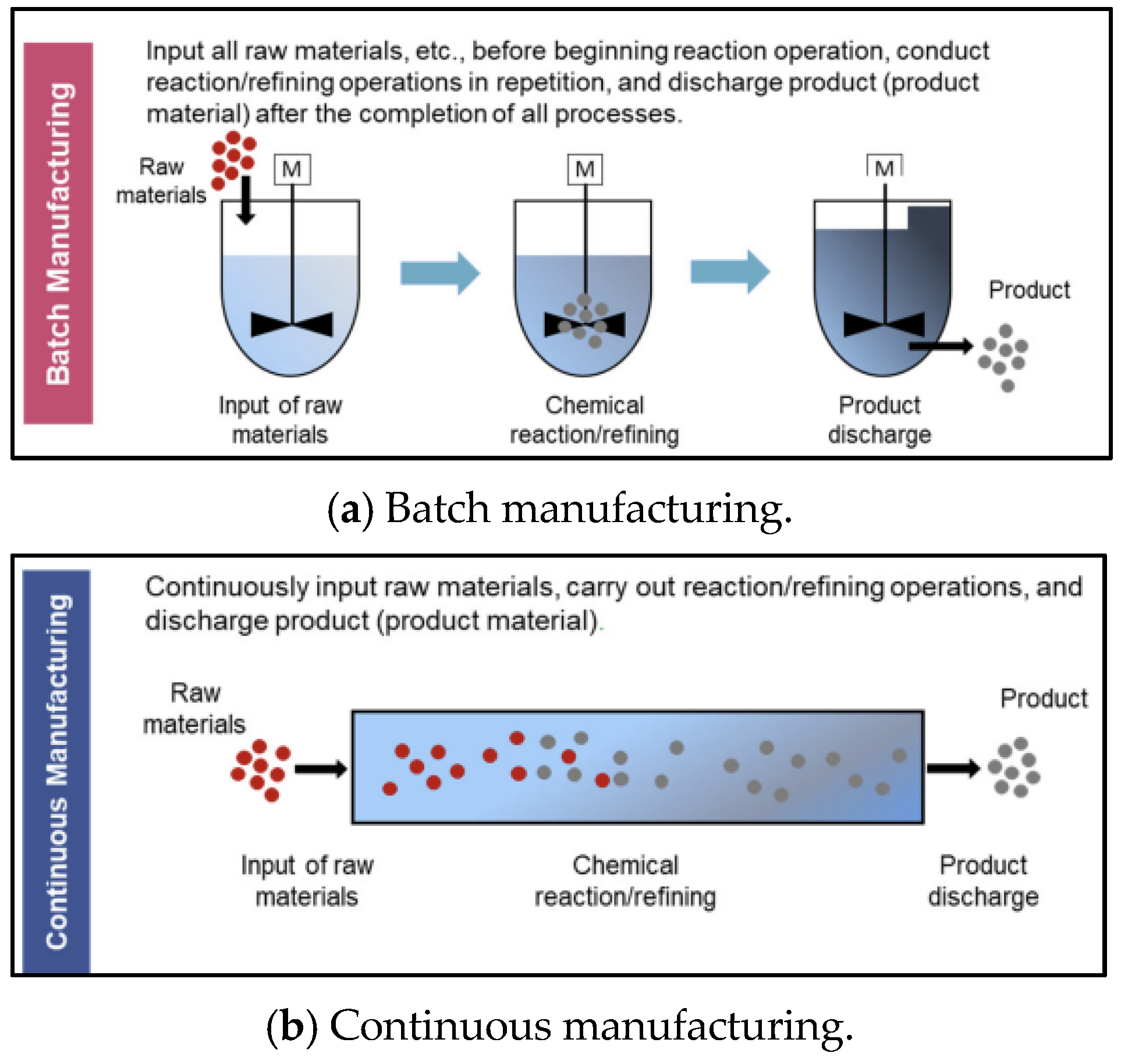
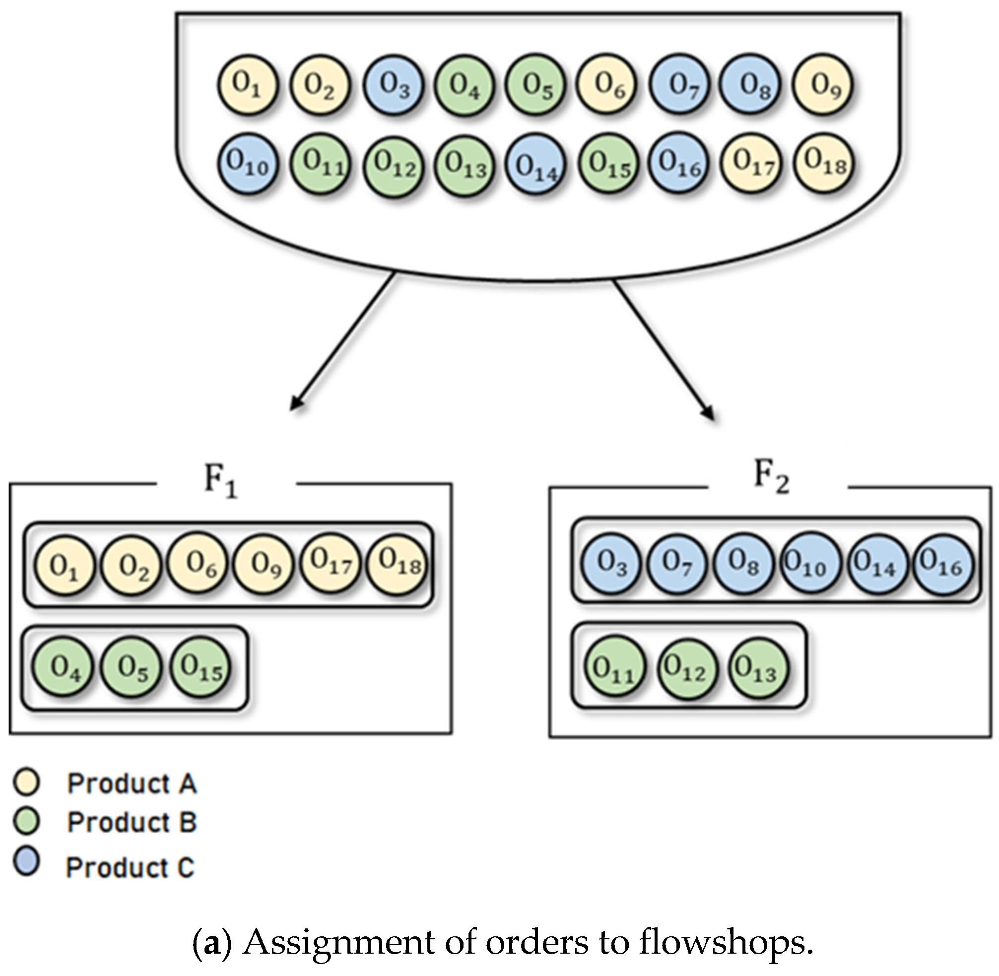
The manufacturing environment consists of multiple flowshops.

(2)

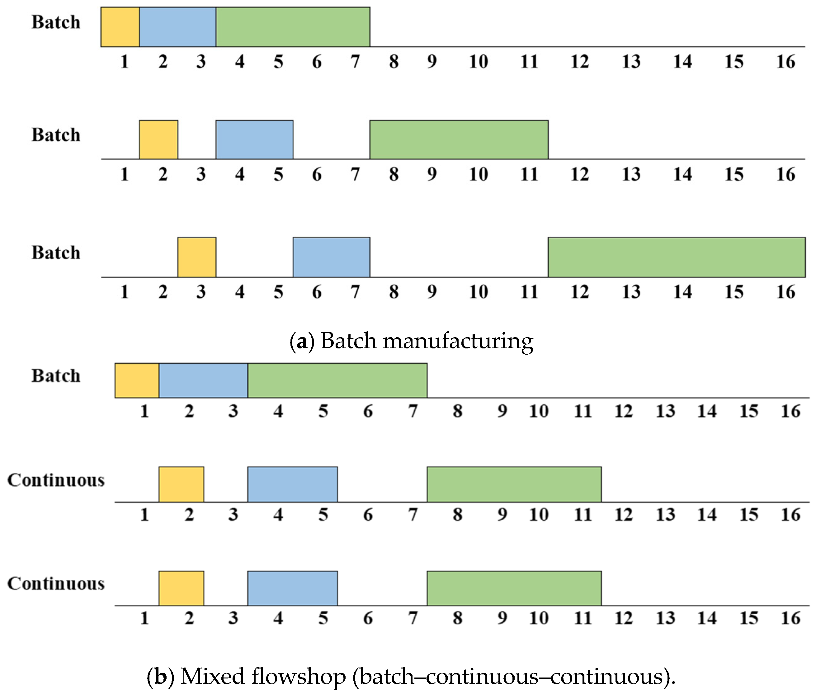
Each flowshop has a single batch process and double continuous processes.

(3)

A product-type sequence-dependent setup exists.

(4)

The processing speed varies for each flowshop and process.

(5)

If two continuous processes are consecutive, for each order, the subsequent process starts and ends after the previous process starts and ends, respectively.

(6)

If at least one of the two consecutive processes is not a continuous process, for each order, the subsequent process starts after the previous process ends.

Figure 4 presents an illustrative example of a feasible solution for the BPMSP-HPMFSs. Figure 4a shows the assignment of orders to the flowshops. There are 18 orders ($O_1$, $O_2$, ⋯, $O_{18}$), each of which is designated one of three product types (A, B, C) and assigned to one of two flowshops ($F_1, F_2$). Six orders ($O_1$, $O_2$, $O_6$, $O_9$, $O_{17}$, $O_{18}$) with product type A and three orders ($O_4$, $O_5$, $O_{15}$) with product type B are assigned to $F_1$. Six orders ($O_3$, $O_7$, $O_8$, $O_{10}$, $O_{14}$, $O_{16}$) with product type C and three orders ($O_{11}$, $O_{12}$, $O_{13}$) with product type B are assigned to $F_2$. The sequencing of assigned orders within each flowshop is shown in Figure 4b. Each flowshop consists of three stages: batch, continuous, and continuous ($I_1^b, I_2^c, I_3^c$). Each flowshop has different processing speeds. The orders with the same product type have the same processing time. In each flowshop, orders with the same product type are processed simultaneously. In $F_1$, three orders ($O_4$, $O_5$, $O_{15}$) with product type B are processed first, followed by six orders ($O_1$, $O_2$, $O_6$, $O_9$, $O_{17}$, $O_{18}$) with product type A. In $F_2$, six orders ($O_3$, $O_7$, $O_8$, $O_{10}$, $O_{14}$, $O_{16}$) with product type C are processed first, followed by three orders ($O_{11}$, $O_{12}$, $O_{13}$) with product type B. To obtain an optimal solution for BPMSP-HPMFS, we present an MILP in Section 3.2.

3.2. Mixed Integer Linear Programming (MILP) Model

The MILP model for the presented problem is as follows:

$$Min\sum \hspace{1em}f\in F, m\in O{T}_{\left|I\right|mf}$$

s.t.

$$C_{\left|I\right|mf}-{Due}_m\le T_{\left|I\right|of},\forall f\in F,m\in O$$

(1)

$$\begin{gathered} {co}_{if}={\sum }_{m,n\in O,p\ne q}{CO}_{ipq}\times z_{mnf},\forall f\in F,i\in I \\ ,p={FT}_m,q={FT}_n \end{gathered}$$

(2)

$$\sum _{f\in F}{y}_{mf}=1,\forall m\in O$$

(3)

$$\sum _{m\in O,{FT}_m=p}{y}_{mf}=x_{pf},\forall f\in F,p\in P$$

(4)

$$\sum _{f\in F}{x}_{pf}=N_p,\forall p\in P$$

(5)

$$\sum _{m\in O}{z}_{mmf}\le 1,\forall f\in F$$

(6)

$$\sum _{m\in O}{z}_{mnf}\le y_{nf},\forall f\in F,n\in O$$

(7)

$$\sum _{n\in O,n\ne m}{z}_{mnf}\le y_{mf},\forall f\in F,m\in O$$

(8)

$${CO}_{ipp}+\left({\displaystyle \frac{{PT}_{ip}}{V_{fi}}}\right)\le C_{imf}+M·\left({}^{\prime }1-z_{mmf}\right),\forall f\in F,i\in I,m\in O,p={FT}_m$$

(9)

$$C_{imf}+\left({\displaystyle \frac{{PT}_{ip}}{V_{fi}}}\right)\le C_{inf}+M·\left(1-z_{mnf}\right),\forall f\in F,i\in I,m,n\in O, m\ne n,p={FT}_m, p={FT}_n$$

(10)

$$C_{imf}+{CO}_{ipq}+\left({\displaystyle \frac{{PT}_{iq}}{V_{fi}}}\right)\le C_{inf}+M·\left(1-z_{mnf}\right),\forall f\in F,i\in I,m,n\in O,m\ne n, p={FT}_m, q={FT}_n, p\ne q$$

(11)

$$C_{imf}+\left({\displaystyle \frac{{PT}_{jp}}{V_{fj}}}\right)\le C_{jmf}+M·\left(1-y_{mf}\right),\forall f\in F,p\in P,m\in O,i\in I^b or j\in I^b, j=i+1, p={FT}_m$$

(12)

$$C_{imf}+\left({\displaystyle \frac{{PT}_{ip}}{V_{fi}}}\right)\times \left(x_{pf}-1\right)\le {CB}_{ipf}+M·\left(1-z_{mmf}\right),\forall f\in F,p\in P,i\in I^b,m\in O,{p=FT}_m$$

(13)

$$C_{inf}+\left({\displaystyle \frac{{PT}_{ip}}{V_{fi}}}\right)\times \left(x_{pf}-1\right)\le {CB}_{ipf}+M·\left(1-z_{mnf}\right),\forall f\in F,p\in P,i\in I^b,m,n\in O,p={FT}_n, p\ne {FT}_m$$

(14)

$${CB}_{ipf}+\left({\displaystyle \frac{{PT}_{jp}}{V_{fj}}}\right)\le C_{jmf}+M·\left(1-z_{mmf}\right),\forall f\in F,p\in P,i\in I^b,m\in O, j=i+1, {p=FT}_m$$

(15)

$${CB}_{ipf}+\left({\displaystyle \frac{{PT}_{jp}}{V_{fj}}}\right)\le C_{jnf}+M·\left(1-z_{mnf}\right), \forall f\in F,p\in P,i\in I^b,m,n\in O, j=i+1, p={FT}_n,p\ne {FT}_m$$

(16)

$$C_{imf}\le C_{jmf}+M·\left(1-y_{mf}\right),\forall f\in F,i,j\in I^c,m\in O,j=i+1,i\ne \left|I\right|$$

(17)

$$C_{imf}-\left({\displaystyle \frac{{PT}_{ip}}{V_{fi}}}\right)\le C_{jmf}-\left({\displaystyle \frac{{PT}_{jp}}{V_{fj}}}\right)+M·\left(1-y_{mf}\right),\forall f\in F,i,j\in I^c,m\in O,j=i+1,i\ne \left|I\right|,p={FT}_m$$

(18)

$$y_{mf}=0 \mathrm{or} 1,\forall f\in F, m\in O$$

(19)

$$z_{mnf}=0 \mathrm{or} 1,\forall f\in F, m,n\in O$$

(20)

$$C_{imf}, {CB}_{ipf}, T_{imf}, {Fco}_{if}, {co}_{if} \ge 0,\hspace{1em}\forall f\in F, p\in P,m\in O, i\in I$$

(21)

Constraint (1) defines the tardiness when an order with product type is completed later than the due date. Constraint (2) refers to the sum of the setup times occurring in all stages of each flowshop. Constraint (3) means that all orders are allocated to the flowshop. Constraint (4) defines the relationship between the order and product type. Constraint (5) means the total number of products allocated to the machine. Constraint (6) means that the first order of each flowshop is less than one. Thus, constraints (7) and (8) define the precedence relationship between orders. Constraint (9) defines the completion time of the first order and, Constraints (10) and (11) define the completion time. Constraint (12) determines the sequence of stages. Constraints (13) and (14) determine the completion of batch production. Constraints (15) and (16) determine the completion of continuous production by utilizing the time of completion of batch production. When the machine is working in a continuous–continuous configuration, it can be divided into three cases. Constraint (17) means that the succeeding process finishes later than the preceding process in a continuous–continuous configuration. Constraint (18) means that the succeeding process starts later than the preceding process in a continuous–continuous configuration.

4. Meta-Heuristic Algorithms

Since the problem of minimizing total tardiness in a single machine environment is NP-hard [24], BPMSP-HPMFSs, an extension of this problem, is also NP-hard. Therefore, BPMSP-HPMFSs cannot be solved through the MILP presented in Section 3 if the size of the problem becomes large. Therefore, to solve a large-sized problem efficiently, we present two population-based meta-heuristic algorithms, GA and PSO, which are widely used in scheduling problems [25,26,27,28]. The same solution representation and decoding procedure are applied to the presented GA and PSO.

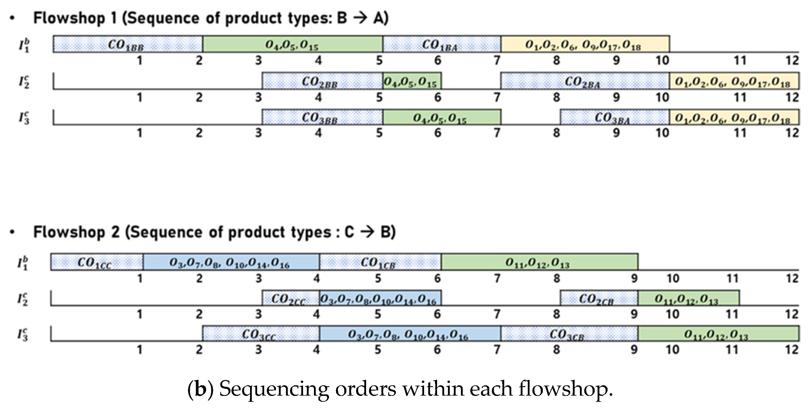
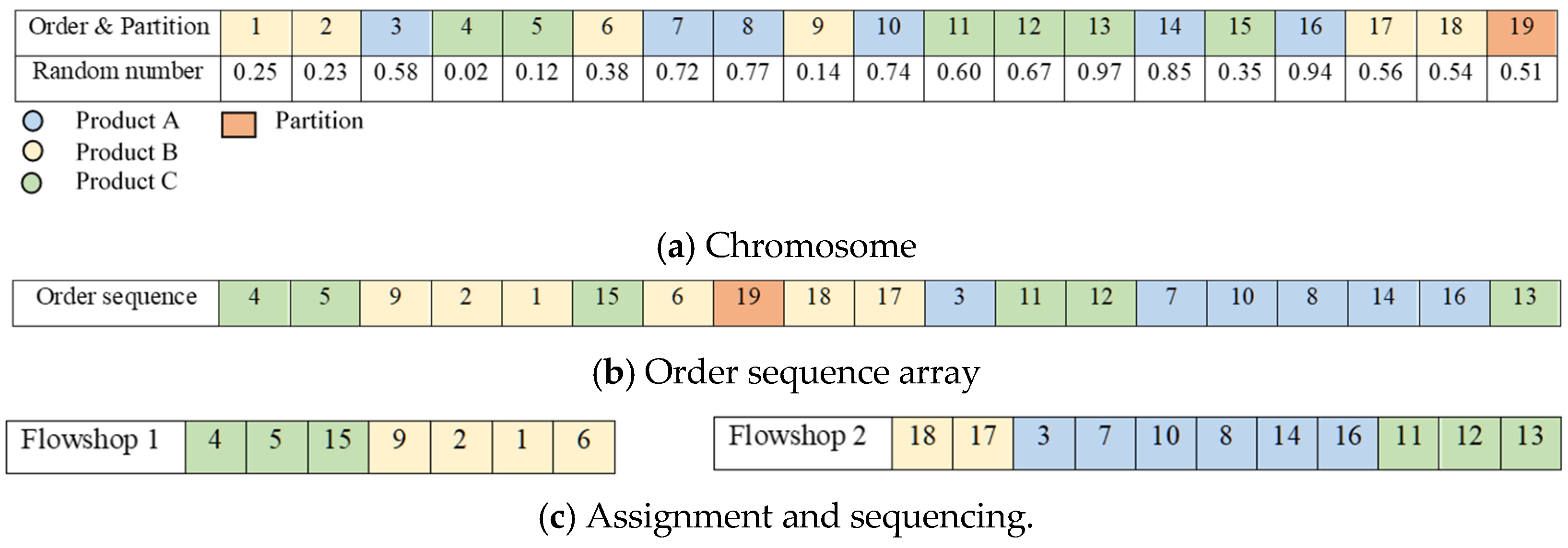
4.1. Solution Representation and Decoding Procedure

The solution is presented as single chromosome with size of $(the number of orders+the number of flowshops-1)$. Figure 5 is an example with eighteen orders, two flowshops, and three product types. In Figure 5a, the size of the chromosome is 19 (=18 + 2 − 1). Index 19, excluding 18 orders, becomes a partition that can assign the orders to the flowshops. The genes in the chromosome are randomly assigned the uniform distribution of real numbers between 0 and 1 ($U(0,1)$). Figure 5a is changed to Figure 5b by the random key method. The smallest of the random numbers in Figure 5a is 0.02 and its index is 4. Therefore, index 4 comes first in Figure 5b. The next smallest number is 0.12, which is index 5 in Figure 5a. In Figure 5b, index 5 comes after 4. In this way, Figure 5b is made. Because index 19 is determined as the partition in Figure 5a, indexes before the ninth position with index 19 in Figure 5b are assigned to flowshop 1, and indexes after the ninth position are assigned to flowshop 2. After the orders are assigned to each flowshop, the sequence between the orders within the flowshop need to be decided. Since the setup is considered as the objective function, it is inefficient to process the same product type multiple times. Therefore, orders of the same product type are processed simultaneously. Then, the sequence of processing the different product types is decided. The method for deciding the sequence of product types is determined as shown in Figure 5b. The sequence of product types in a flowshop follows the sequence in which the product type appears first. The first order processed in flowshop 1, order 4, has product type B. Therefore, orders with product type B are processed first in flowshop 1. Among the orders whose product type is not B, order 9 comes first. The product type in order 9 is A. Thus, product type A is processed after product type B. In flowshop 2, order 18 with product type A is processed first, and order 3 with product type C and order 11 with product type B are processed last. The sequence between orders within the same product type follows the sequence of orders in Figure 5b. Figure 5c shows that the assignment and sequencing of the orders within each flowshop have been completed. This solution representation and decoding procedure are applied to both GA and PSO.

4.2. Genetic Algorithm (GA)

GA is one of the population-based meta-heuristics inspired by natural selection and genetics. Through mutation and crossover, some of the parents and offspring are selected and passed on to new generations, which converge on the best chromosomes. First, chromosomes are initialized with the uniform distribution of real numbers between 0 and 1 (U(0, 1)). One-cut point crossover and uniform mutation, which had the best performance in BPMSP-HPMFSs during our preliminary experiments, are used as genetic operators. One-cut point crossover selects two chromosomes and randomly determines genes to start tweaking. Then, the selected two chromosomes tweaked based on the determined gene. Uniform mutation is a random change in the numeric value of a gene to U(0, 1). In the decoding procedure, the objective function value is obtained through the presented decoding process. In the selection, the second of the next generations is selected through the roulette wheel method. The GA procedure is shown in Algorithm 1.

Algorithm 1: GA

Input: population size ($S_p$), generation size ($S_g$), crossover rate ($p_c$), mutation rate ($p_m$)

Output: total tardiness

Initialization: Generate a random initial population through $U(0,1)$

While $g$ $\le$ $S_g$

For $i$ $\le$ $S_p$

If $U(0,1)$ < $p_c$

$j$ $=i$

For $j$ $\le$ $S_p$

If $U(0,1)$ < $p_c$

Conduct the crossover of the ith chromosome and jth chromosome

End if

End for

End if

End for

For $i$ $\le$ $S_p$

For $n$ $\le$ $N$

If $U(0,1)$ < $p_m$

Conduct the mutation operation

End if

End for

End for

Decode the chromosome and compute the objective function value (see Figure 5)

Conduct the roulette wheel selection

$g$ = $g+1$

End While

4.3. Particle Swarm Optimization (PSO)

PSO is also one of the population-based meta-heuristics that mimics the movement of groups. In initialization, the positions and velocities receive $U(0,1)$ and form a one-dimensional array. In the decoding procedure, the objective function value is obtained by the decoding process, which can be presented similarly to that of GA. After the decoding procedure, the best solution for particles $\left(P_i\right)$ and the global best solution $\left(P_g\right)$ are updated. The velocity $\left(v_i\right)$ and position $\left(X_i\right)$ of each particle are updated using Equations (22) and (23) based on $P_i$ and $P_g$, respectively.

$$v_i\leftarrow v_i+c_1 U\left(0, 1\right)\times \left(P_i-X_i\right)+c_2\times U\left(0, 1\right)\times \left(P_g-X_i\right),$$

(22)

$$X_t^i\leftarrow X_{t-1}^i+v_t^i.$$

(23)

The PSO procedure is shown in Algorithm 2.

Algorithm 2: PSO

Input: iteration ($Iter$), swarm size ($S_p$), weight ($W$), acceleration weight ($c_1$), and ($c_2$)

Output: total tardiness

Initialization: Generate a random initial population through $U(0,1)$

While $g$ $\le$ $Iter$

For $i$ $\le$ $S_p$

Decode the chromosome and compute the objective function value (see Figure 5)

If $f\left(X_i\right)$ < $f\left(P_i\right)$

$P_i=X_i$

End if

If $f\left(X_i\right)$ < $f\left(P_g\right)$

$P_g=X_i$

End if

End for

For $i$ $\le$ $S_p$

$v_i{=W\times v}_i+c_1\times U\left(0,1\right)\times \left(P_i-X_i\right)+c_2\times U\left(0,1\right)\times \left(P_g-X_i\right)$

$X_t^i=X_{t-1}^i+v_t^i$

End for

$g=g+1$

End While

5. Computational Experiments

In this section, we conduct experiments to evaluate the performance of the two proposed meta-heuristic algorithms. The experiments are divided into instances of small- and large-size problems depending on the combination of parameters that affect the complexity of the problem. The parameters are the number of product types ($\left|P\right|$), the number of orders for each product type ($N_p$), and the number of flowshops ($\left|F\right|$). In the experiment with instances of small-size problems, the performance of GA and PSO was verified by comparing them with the optimal solution obtained by the MILP model. In the experiment with instances of large-size problems, the performance of the GA and PSO were compared in relation to one another. The MILP and the two meta-heuristic algorithms were implemented using the CPLEX solver 22.11.1 and C#, respectively. All experiments were performed using PCs with 13th Gen Intel(R) Core™ i7-13700KF 3.40 GHz CPU.

5.1. Design of Experiments

Instances of small- and large-size problems were generated according to the combination of $\left|F\right|$, $N_p$, and $\left|P\right|$. ${Due}_o$ is set by changing the estimate of $C_{max} \left(\widehat{C_{max}}\right)$ and the proportion of tardy orders ($\tau$), where $C_{max}$ is the makespan. $\widehat{C_{max}}$ is calculated as shown below:

$$\widehat{C_{max}}=r\times \left[\left\{{\displaystyle \frac{\frac{{PT}_{pi}^{UB}+{PT}_{pi}^{LB}}{2}}{\frac{V_{fi}^{UB}+V_{fi}^{LB}}{2}}}\times {\displaystyle \frac{N_p}{\left|F\right|}}+{\displaystyle \frac{{CO}_{ipq}^{UB}+{CO}_{ipq}^{LB}}{2}}\right\}+\left\{\left(\left({\displaystyle \frac{{PT}_{pi}^{UB}+{PT}_{pi}^{LB}}{\frac{V_{fi}^{UB}+V_{fi}^{LB}}{2}}}\right)\times {\displaystyle \frac{N_p}{\left|F\right|}}+\left({CO}_{pi}^{UB}+{CO}_{pi}^{LB}\right)\right)\times {\displaystyle \frac{2\left|P\right|}{3}}\right\}\right]$$

(24)

The first term is the completion time for the first product type in the batch process. The processing time and setup time required to calculate the completion time are the average of the upper bound and lower bound, respectively. The second term is the completion time in continuous manufacturing. According to Figure 5, when two continuous processes appear in succession, the completion time of the subsequent process is determined by the process with the longer processing time among the two processes, so the second term is multiplied by ${\displaystyle \frac{2\left|P\right|}{3}}$. The sum of the first term and the second term is the average value of $C_{max}$. ${Due}_o$ is generated from the discrete distribution of $U\left(\right(1-\mathsf{\tau })\times \widehat{C_{max}}\times 0.25,(1-\mathsf{\tau })\times \widehat{C_{max}}\times 1.75$).

Table 2. Instances of problems for small- and large-size experiments.

	$\left|\mathit{F}\right|$	$\left|\mathit{P}\right|$	${\mathit{N}}_{\mathit{p}}$	${\mathit{V}}_{\mathit{f}\mathit{i}}$	${\mathit{C}\mathit{O}}_{\mathit{i}\mathit{p}\mathit{q}}$	${\mathit{P}\mathit{T}}_{\mathit{p}\mathit{i}}$	${\mathit{D}\mathit{u}\mathit{e}}_{\mathit{o}}$
Small-size instances	{2,3}	{3,4}	{2,3,4}	$U(1,2.5)$	$U(54,108)$	$U(30, 120)$	$U\left(\right(1-\tau )\times \widehat{C_{max}}\times 0.25,$ $(1-\tau )\times \widehat{C_{max}}\times 1.75$)
Large-size instances	{5,6,7}	{10,11,12}	{30,35,40}

Some parameters refer to other studies: $V_{fi}$ [29], ${CO}_{ipq}$ [8].

summarizes the values of the problem parameters.

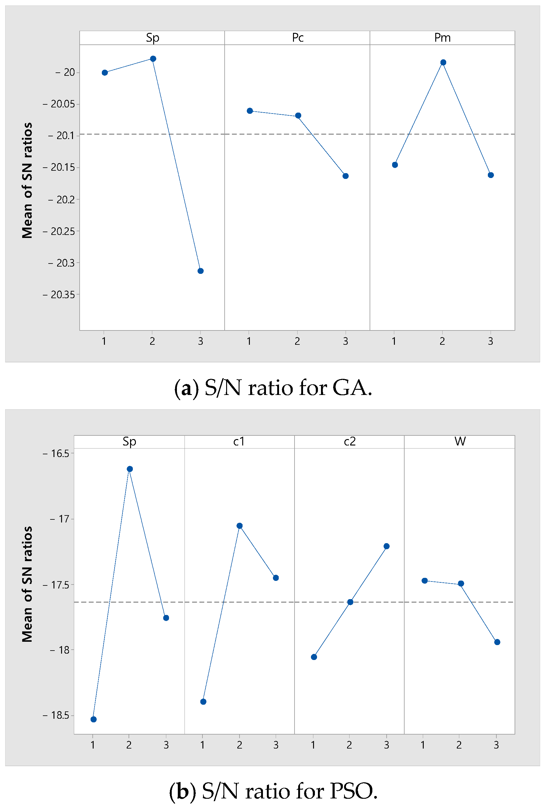
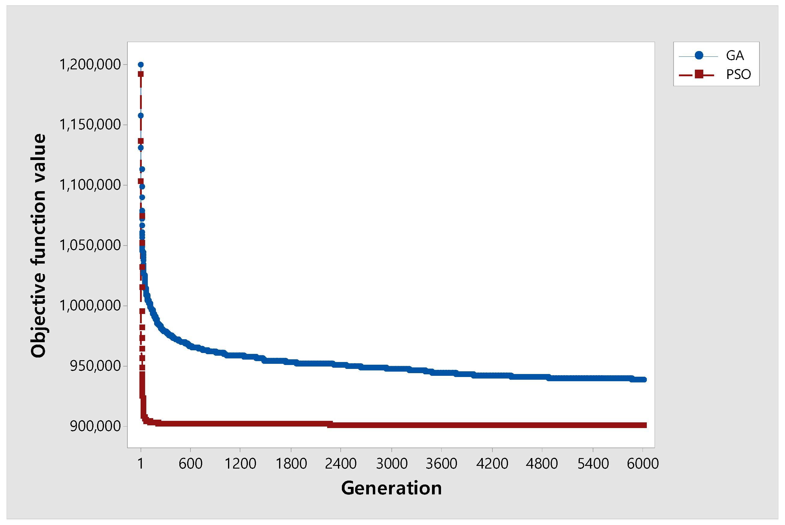
5.2. Calibration of Meta-Heuristic Parameters

Calibrating meta-heuristic algorithm parameters significantly affects the performance of algorithms. The Taguchi method was used to find the best parameter combinations for the GA and PSO. In the Taguchi method, the S/N ratio is used to find optimal conditions by simultaneously considering performance and volatility. Since the objective function of BPMSP-HPMFSs is the smaller the better, the S/N ratio is calculated as follows.

$$S/N ratio=-10·\log ({\displaystyle \frac{1}{n}}·\sum _{i=1}^n{obj}_i^2)$$

(25)

where $n$ is the number of combinations of parameters for each GA and PSO.

Table 3. Values for each level of GA and PSO parameters tuned using the Taguchi method.

Level	GA			PSO
	${\mathit{S}}_{\mathit{p}}$	${\mathit{P}}_{\mathit{c}}$	${\mathit{P}}_{\mathit{m}}$	${\mathit{S}}_{\mathit{p}}$	${\mathit{c}}_1$	${\mathit{c}}_2$	$\mathit{W}$
1	$\left|O\right|\times 0.095$	0.1	0.3	$\left|O\right|\times 0.095$	1	1	0.3
2	$\left|O\right|\times 0.1$	0.2	0.5	$\left|O\right|\times 0.1$	2	2	0.5
3	$\left|O\right|\times 0.105$	0.3	0.7	$\left|O\right|\times 0.105$	3	3	0.7

shows the values for each level of GA and PSO parameters tuned through the Taguchi method. The $S_g$ of GA and the $Iter$ of PSO are fixed as 6000. Figure 6 shows the S/N ratio for each parameter value for GA and PSO. In Figure 6, the level with the largest S/N ratio for each parameter is selected. For GA, the best $S_p$, $P_c$, and $P_m$ are $(\left|O\right|\times 0.1)$, 0.1, and 0.5. For PSO, the best $S_p$, $c_1$, $c_2$, and $W$ are $(\left|O\right|\times 0.1)$, 2, 3, and 0.3.

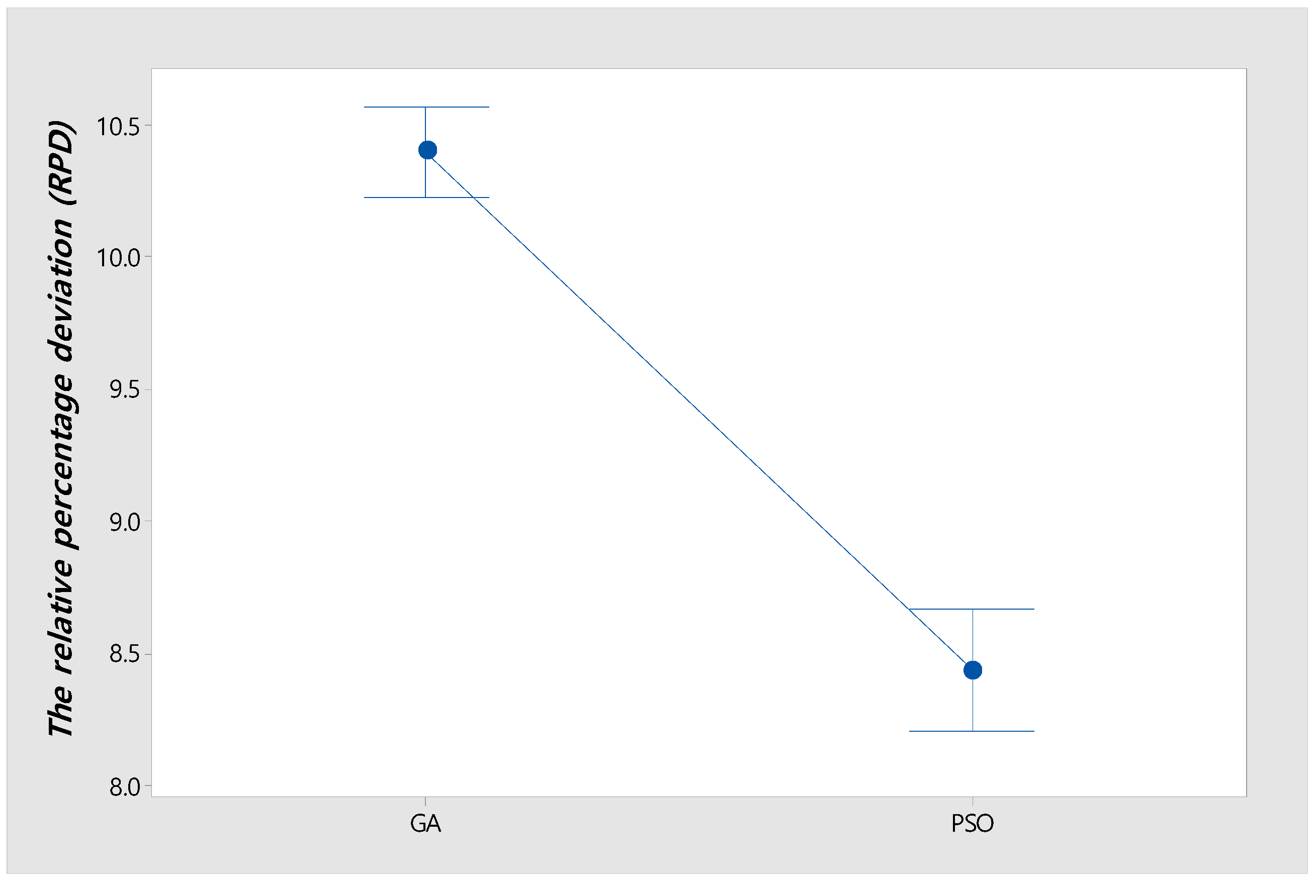
5.3. Experimental Results in the Small-Size Problem Instances

In instances of small-size problems, we compare the absolute percentage deviation (APD) and CPU time of the MILP model, GA, and PSO with $\mathsf{\tau }=0.7$. APD is calculated as follows:

$$APD\left(\%\right)={\displaystyle \frac{{Alg}_{sol}-Opt}{Opt}}\times 100$$

(26)

where ${Alg}_{sol}$ denotes the objective function value generated by the meta-heuristic and $Opt$ denotes the objective function value of the optimal solution obtained by CPLEX with a time limit of 3600 s. GA and PSO are tested with 30 replications for each instance. As shown in

Table 4. Computational results for small problems.

$\left|\mathit{F}\right|$	$\left|\mathit{P}\right|$	${\mathit{N}}_{\mathit{p}}$	MILP		GA		PSO
			${\mathit{O}\mathit{p}\mathit{i}\mathit{m}\mathit{a}\mathit{l}}_{\mathit{s}\mathit{o}\mathit{l}}$	CPU	APD(%)	CPU	APD (%)	CPU
2	3	2	607.54	1.31	0.00	8.93	0.02	6.09
		3	661.03	0.06	0.92	5.29	0.92	3.75
		4	967.18	18.61	3.35	18.86	4.03	12.92
	4	2	780.72	2.02	1.73	10.96	1.77	7.67
		3	883.3	279.56	3.05	18.83	3.77	13.06
		4	N/A	3600.00	N/A	32.83	N/A	22.24
3	3	2	498.47	1.58	0.00	9.81	0.22	6.95
		3	642.26	0.17	0.64	6.03	0.69	4.39
		4	892.67	73.61	2.57	20.68	3.07	14.5
	4	2	718.3	4.05	0.00	12.32	0.60	8.78
		3	808.76	356.2	3.47	18.73	4.75	14.26
		4	N/A	3600.00	N/A	35.55	N/A	23.73
avg.				661.43	1.57	16.57	1.98	11.54

, CPELX cannot find a feasible solution with limited time for instances with both $\left|P\right|$ and $N_p$ larger than 3, which are marked as N/A. Also, the average APDs for GA and PSO excluding instances marked as N/A are $1.57\mathrm{\%}$ and $1.98\mathrm{\%}$, respectively. This means that GA and PSO find efficient solutions compared to the solution obtained by CPLEX. Therefore, meta-heuristics are necessary to find efficient solutions within a limited time frame in large-size problems.

5.4. Experimental Results in Instances of Large-Size Problems

In large-size problems, we run three experiments by changing $\tau$. We compare the relative percentage deviation (RPD) and CPU time of the GA, and PSO with $\tau =0.3, 0.5, \mathrm{a}\mathrm{n}\mathrm{d} 0.7$. RPD is as follows:

$$RPD(\mathrm{\%})={\displaystyle \frac{{Alg}_{sol}-{B\mathrm{e}\mathrm{s}\mathrm{t}}_{sol}}{{B\mathrm{e}\mathrm{s}\mathrm{t}}_{sol}}}\times 100$$

(27)

where ${Best}_{sol}$ denotes the best objective function value obtained using GA and PSO. GA and PSO were tested with 30 replications for each instance. The experimental results according to $\tau$ are shown in

Table 5. Computational results for large problems.

			$\mathsf{\tau } = 0.3$				$\mathsf{\tau } = 0.5$				$\mathsf{\tau } = 0.7$
			GA		PSO		GA		PSO		GA		PSO
$\left|\mathit{F}\right|$	$\left|\mathit{P}\right|$	${\mathit{N}}_{\mathit{p}}$	RPD (%)	CPU	RPD (%)	CPU	RPD (%)	CPU	RPD (%)	CPU	RPD (%)	CPU	RPD (%)	CPU
5	10	30	23.94	47.23	21.13	44.53	8.87	47.20	6.17	44.28	8.33	47.49	7.20	44.09
		35	19.51	46.65	17.81	44.87	12.97	46.84	11.64	44.04	6.44	46.86	5.33	44.13
		40	20.90	46.28	20.35	44.38	18.81	46.20	14.84	44.12	8.64	46.46	7.68	43.95
	11	30	22.75	70.39	17.10	66.41	16.39	70.58	15.04	66.62	4.82	71.05	3.30	66.12
		35	13.44	69.59	12.56	66.47	11.29	69.36	9.58	65.69	5.16	69.84	3.70	65.69
		40	27.80	68.81	23.37	65.85	13.02	68.51	13.06	65.63	8.26	69.07	6.63	65.61
	12	30	15.13	99.95	11.56	94.28	14.99	99.67	11.10	93.52	7.06	100.91	4.04	93.94
		35	13.25	98.00	9.97	93.51	11.24	98.11	8.81	92.91	8.26	98.72	5.69	92.88
		40	24.32	96.82	17.47	92.96	17.17	97.00	16.45	92.73	8.32	97.60	6.89	93.18
6	10	30	22.50	60.22	17.39	56.72	9.80	60.19	6.18	56.30	6.34	60.20	4.90	56.56
		35	18.11	59.20	15.93	56.44	10.95	59.48	10.25	56.13	6.27	59.42	5.94	56.44
		40	18.77	58.77	18.61	56.50	12.36	58.89	11.55	56.23	7.81	58.82	6.42	56.08
	11	30	18.14	88.94	14.38	83.82	8.19	89.47	6.09	83.50	5.00	89.21	3.76	83.74
		35	12.44	87.04	12.56	83.27	10.70	87.68	8.88	82.37	5.69	87.61	3.73	82.43
		40	17.29	85.94	19.26	82.90	12.39	86.93	7.61	82.75	6.67	86.27	6.80	82.53
	12	30	21.94	128.49	17.67	120.53	17.41	127.85	12.76	119.95	5.57	128.93	3.11	119.97
		35	17.36	125.94	13.38	118.78	8.42	125.83	5.23	119.40	7.09	126.12	4.87	119.08
		40	27.95	123.72	19.77	118.19	11.67	124.13	10.75	119.57	5.81	124.60	4.62	118.09
7	10	30	16.71	75.33	15.13	71.40	14.24	75.48	11.75	70.74	5.36	75.38	3.76	70.66
		35	26.77	76.49	21.31	69.75	11.45	74.17	9.91	70.10	11.94	74.43	9.31	70.84
		40	23.78	73.43	19.46	70.71	10.02	73.30	7.71	70.18	5.29	73.37	3.30	70.37
	11	30	13.04	112.75	9.60	106.33	9.09	113.50	6.48	106.31	6.44	113.79	5.82	105.85
		35	18.99	110.81	14.51	105.09	14.66	111.02	12.32	105.19	7.78	111.58	5.55	104.67
		40	22.23	109.81	17.38	105.28	11.70	109.62	9.34	104.49	7.62	109.83	4.46	103.88
	12	30	16.10	161.78	11.97	151.90	8.22	160.70	4.55	150.95	3.96	160.76	2.09	150.96
		35	16.61	157.53	10.56	149.16	9.27	157.04	6.99	149.06	7.19	157.32	4.89	148.75
		40	16.04	154.81	11.94	147.50	9.62	154.71	5.76	148.35	8.46	154.79	5.63	147.32
Average			19.47	92.40	16.01	87.69	12.03	92.35	9.66	87.45	6.87	92.61	5.16	87.33

. For $\tau =0.3$, the average of RPDs for GA and PSO are 19.47 and 16.01, respectively. For $\tau =0.5$, the average of RPDs for GA and PSO are 12.03 and 9.66, respectively. For $\tau =0.7$, the average of RPDs for GA and PSO are 6.87 and 5.16, respectively. In all settings of $\tau$, PSO has a better average RPD and a shorter CPU time than GA under the meta-heuristic parameters described in Section 5.2.

A convergence test was performed to analyze the performance differences for GA and PSO. For each $\tau$, $N_p$ and $\left|P\right|$ are fixed as 12 and 40, respectively, and instances with $\left|F\right|=5, 6, \mathrm{a}\mathrm{n}\mathrm{d} 7$ were selected, and the experiment was repeated five times for nine data points. Figure 7 shows that PSO has a better performance and converges faster than GA.

Figure 8 shows an interval plot of GA and PSO with a 95% confidence level for all instances in Table 5. Also, it shows that the confidence intervals between GA and PSO do not overlap. Thus, the difference in RPD between GA and PSO is statistically significant.

6. Sensitivity Analysis

To obtain managerial insights into the BPMSP-HPMFSs, we conducted three sensitivity analysis experiments. In this section, we define the total cost of the production schedule as the sum of setup and tardiness costs and analyze it. In Section 6.1, we investigate the changes in total, setup, and tardiness costs as the number of flowshops increases. In Section 6.2, we examine the change in the percentage of orders completed before the due date as the number of product types is varied. In Section 6.3, we investigate the changes in the costs as the decrease in the number of product types under the fixed number of total orders. In Section 6.4, we analyze the effect of delays time in real-world continuous processes on the objective function, total tardiness.

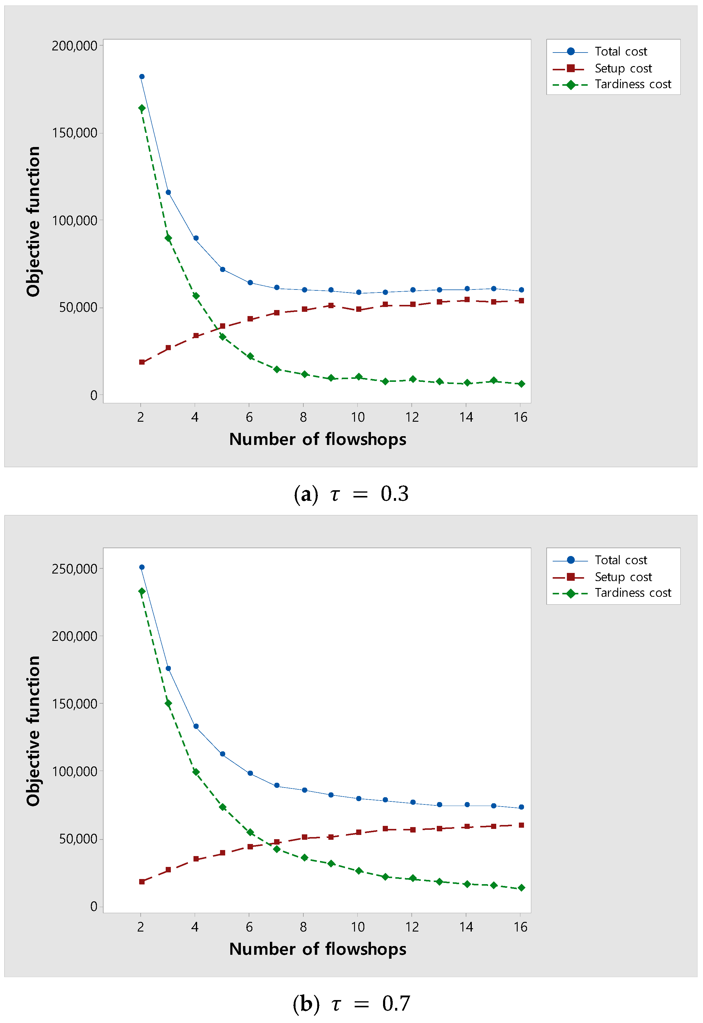
6.1. Changes in the Total, Setup, and Tardiness Costs as the Number of Flowshops Increases

As the number of flowshops increases, the tardiness cost is expected to decrease and the setup cost to increase because the number of orders assigned to each flowshop decreases. An experiment was performed to investigate changes in the total costs due to changes in tardiness and setup costs as the number of flowshops increased. Figure 9 shows changes in the total, setup, and tardiness costs as an increase in the number of flowshops. Figure 9a,b are experiments for instances with $\tau$ of 0.3 and 0.7, respectively. In both Figure 9a,b, as the number of flowshops increases, the total cost decreases and then converges. In Figure 9a, where $\tau$ is relatively small, the tardiness cost rapidly decreases and converges as the number of flowshops increases because the due date of orders is loose. On the other hand, in Figure 9b, where $\tau$ is relatively large, the tardiness cost slowly decreases and converges as the number of flowshops increases because the due date of orders is tight. As a result, the experiment suggests the appropriate number of flowshops according to $\tau$.

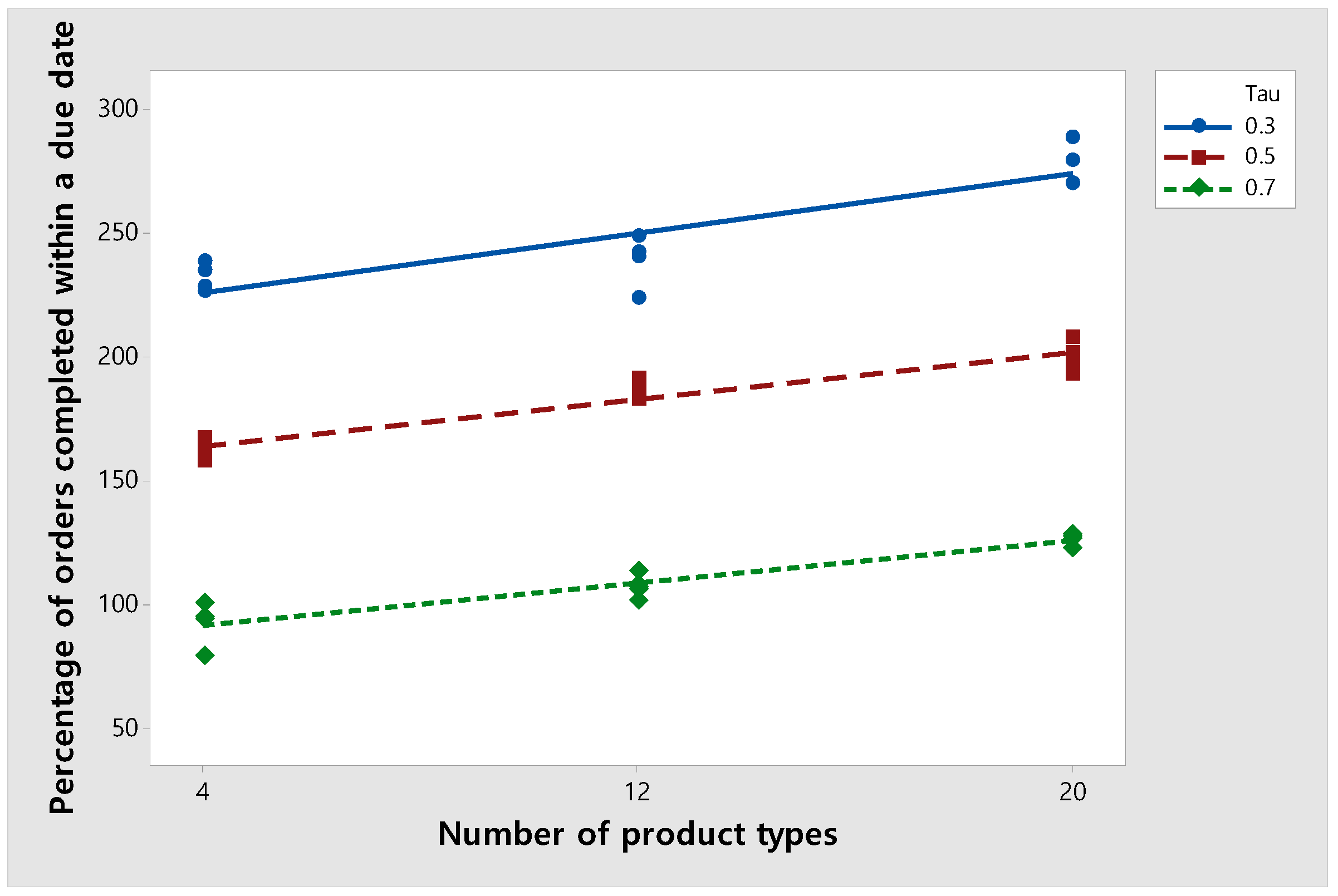
6.2. Change in the Percentage of Orders Completed Before the Due Date as the Number of Product Types Is Varied

In this section, we examine the percentage of orders completed before the due date as the number of product types is varied. Figure 10 shows the percentage of orders completed within a due date when the number of product types changes. In this experiment, the number of total orders is fixed at 420. When $\tau$ is 0.3, 0.5, and 0.7, the percentage of orders completed before a due date increases as the number of product types increases. This is because when the number of product types within a fixed number of orders is low, the algorithm tends to process orders with the same type at the same time to reduce the setup time. On the other hand, when the number of product types is large, the tendency to reduce the setup time is relatively reduced, and orders with fast-approaching due dates are completed first. This hypothesis is verified through the final sensitivity analysis experiment outlined in Section 6.3.

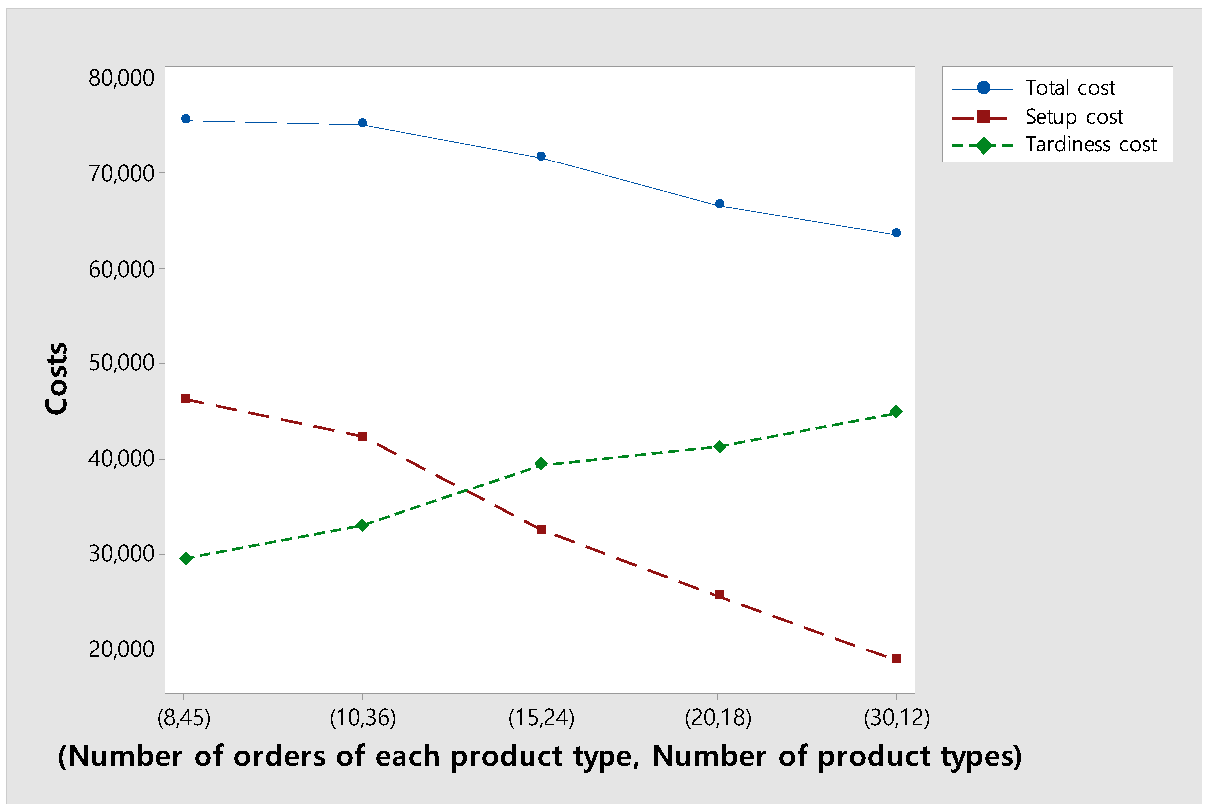
6.3. Change in the Total, Setup, and Tardiness Costs as the Number of Product Types Within a Fixed Number of Total Orders Decreases

Figure 11 shows changes in the total, setup, and tardiness costs as the number of product types within a fixed number of total orders decreases. As expected, as the number of product types decreases, setup costs decrease. On the other hand, in return for reducing the setup cost, the tardiness cost increases as the percentage of orders completed before a due date decreases. As a result, total costs decrease as the number of product types decreases. This is because when the number of product types decreases, it is possible to decide whether to process orders of the same product type together to reduce setup costs or process urgent orders first to reduce tardiness costs, increasing the degree of freedom in decision-making.

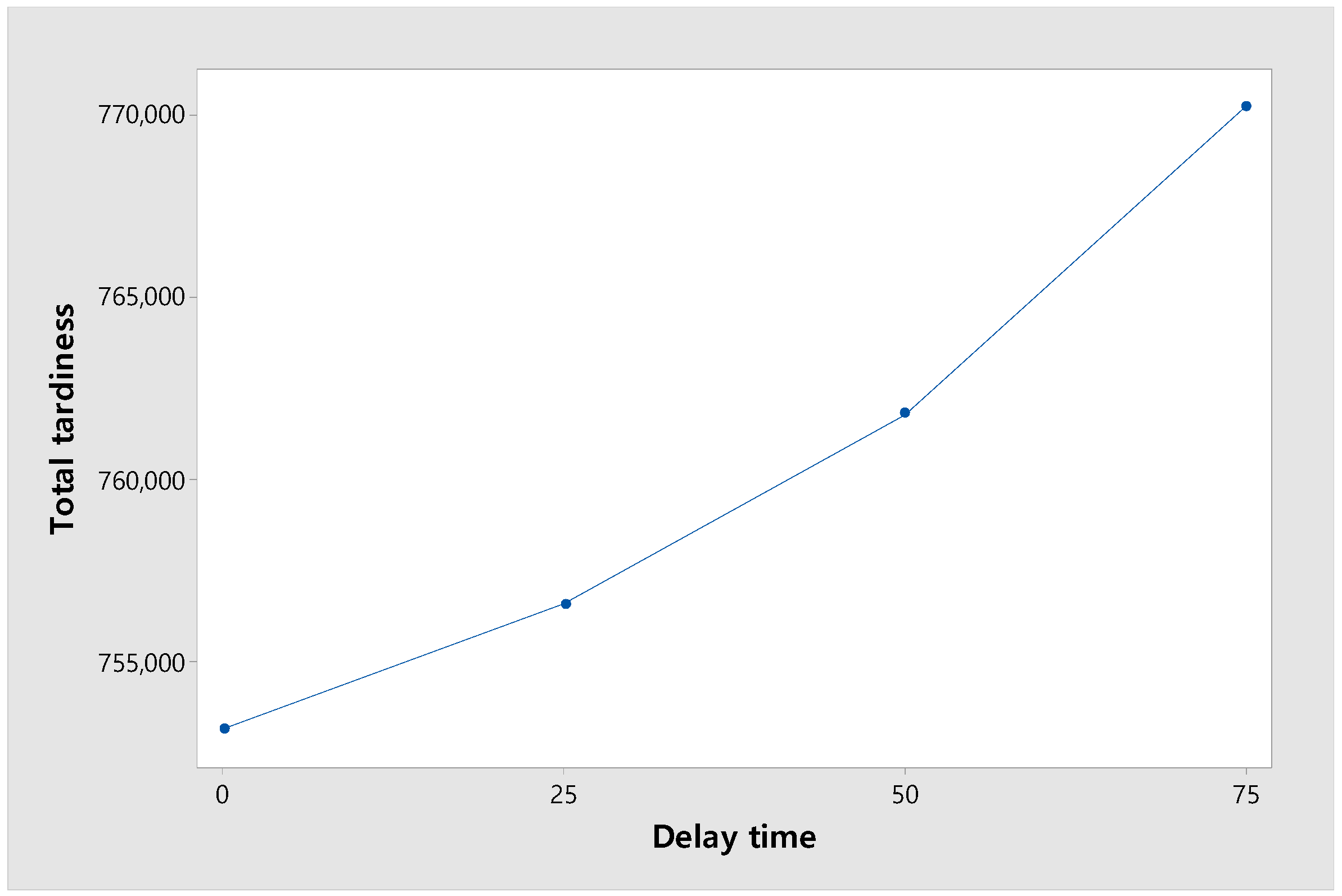
6.4. Change in the Effect of Delays Occurring in Real-World Continuous Processes on the Total Tardiness

In real-world continuous process, raw materials are injected into the process operation continuously, and the product (product material) is discharged continuously and sequentially after a certain time following chemical reaction, refining, and product discharge [4]. We investigate how a delay occurring in a real continuous process affects the objective function, total tardiness. Figure 12a,b show an example of a Gantt chart for the mixed flowshop manufacturing process with and without considerations of delays, respectively.

In Figure 12a, delay time is not considered, so the intermediate goods, which are the output of the flowshop, are immediately input into the third process (the second continuous process) after the second process (the first continuous process) is completed. On the other hand, in Figure 12b, the delay time is considered, so the intermediate goods, which are the output of the second process, are input to the third process following a delay in the second process. In Figure 12a, all orders are completed before the delivery date, but in Figure 12b, the completion times of $O_1$ and $O_3$ exceed the due date, resulting in tardiness.

Figure 13 shows the change in total tardiness according to the delay time. The experiment was conducted with four levels of delay time, [0, 25, 50, 75], and the objective function, total tardiness, showed an increasing trend. When total tardiness was increased from 0 to 25, the number of orders exceeding the due date was relatively small, so the increase in total tardiness was small. However, as it increased from 25 to 50 and from 50 to 75, the number of orders exceeding the due date increased, so the increase became larger.

7. Conclusions

This study addressed a biopharmaceutical manufacturing scheduling problem with heterogeneous parallel mixed flowshops. The objective function was to minimize the total tardiness. To obtain the optimal solution, the mixed-integer linear programming model was developed. To efficiently solve the problem, two meta-heuristic algorithms, the genetic algorithm and particle swarm optimization, were developed. In the experiment for small-size problems, the mixed-integer linear programming model and the proposed meta-heuristic algorithms obtained the optimal and near-optimal solutions, respectively. In the experiments for large-size problems, three experiments were conducted by changing the proportion of tardy orders with tardiness out of total orders. Particle swarm optimization showed a better performance than the genetic algorithm in all three experiments. A sensitivity analysis was conducted for particle swarm optimization, which showed a better performance. We obtained some managerial insights through the sensitivity analysis. First, we found that the total cost decreases and converges as the number of flowshops increases. Second, the percentage of orders completed by a due date increases as the number of product types increases. Third, setup and total costs decrease as the number of product types decreases. Finally, a discharge delay time occurring in a real continuous process increases the objective function, total tardiness.

In future studies, we will conduct research with experiential validation using real-world data or collaboration with industry partners because no real data on the biopharmaceutical production process were used in this study. In this study, we developed the two meta-heuristic algorithms suitable for a static environment of pharmaceutical scheduling. On the other hand, state-of-the-art algorithms for use in the machine learning field are needed to solve the pharmaceutical scheduling problem in a dynamic environment. So, we will develop state-of-the-art algorithms for use in the machine learning field using empirical scheduling data suitable for the dynamic environment of pharmaceutical scheduling problems. We will also conduct a comparative experiment with other population-based meta-heuristic algorithms such as the chaotic gravitational search algorithm, ant colony optimization, imperialist competition algorithm, gray wolf optimization, and the whale optimization algorithm.

References

1. Kesik-Brodacka, M. Progress in Biopharmaceutical Development. Biotechnol. Appl. Biochem. 2018, 65, 306–322. [Google Scholar] [CrossRef] [PubMed]
2. Liu, S.; Farid, S.S.; Papageorgiou, L.G. Integrated Optimization of Upstream and Downstream Processing in Biopharmaceutical Manufacturing under Uncertainty: A Chance Constrained Programming Approach. Ind. Eng. Chem. Res. 2016, 55, 4599–4612. [Google Scholar] [CrossRef]
3. Casola, G.; Sugiyama, H. Uncertainty-Conscious Methodology for Process Performance Assessment in Biopharmaceutical Drug Product Manufacturing. AIChE J. 2018, 64, 1272–1284. [Google Scholar] [CrossRef]
4. Inada, Y. Continuous Manufacturing Development in Pharmaceutical and Fine Chemicals Industries; MITSUI & Co., Ltd.: Tokyo, Japan, 2019. [Google Scholar]
5. Chatterjee, S. FDA Perspective on Continuous Manufacturing. In Proceedings of the IFPAC Annual Meeting, Baltimore, MD, USA, 22–25 January 2012; pp. 22–25. [Google Scholar]
6. Hernandez, R. Continuous Manufacturing: A Changing Processing Paradigm. BioPharm Int. 2015, 28, 20–27. [Google Scholar]
7. Lee, S.L.; O’Connor, T.F.; Yang, X.; Cruz, C.N.; Chatterjee, S.; Madurawe, R.D.; Moore, C.M.V.; Yu, L.X.; Woodcock, J. Modernizing Pharmaceutical Manufacturing: From Batch to Continuous Production. J. Pharm. Innov. 2015, 10, 191–199. [Google Scholar] [CrossRef]
8. Kopanos, G.M.; Méndez, C.A.; Puigjaner, L. MIP-Based Decomposition Strategies for Large-Scale Scheduling Problems in Multi-product Multistage Batch Plants: A Benchmark Scheduling Problem of the Pharmaceutical Industry. Eur. J. Oper. Res. 2010, 207, 644–655. [Google Scholar] [CrossRef]
9. Kim, J.; Kim, J.; Lee, T.; Lee, I.; Moon, I. A Heuristic-Embedded Scheduling System for a Pharmaceutical Intermediates Manufacturing Plant. Ind. Eng. Chem. Res. 2010, 49, 12646–12653. [Google Scholar] [CrossRef]
10. Raaymakers, W.H.M.; Hoogeveen, J.A. Scheduling Multipurpose Batch Process Industries with No-Wait Restrictions by Simulated Annealing. Eur. J. Oper. Res. 2000, 126, 131–151. [Google Scholar] [CrossRef]
11. Kabra, S.; Shaik, M.A.; Rathore, A.S. Multi-Period Scheduling of a Multi-Stage Multi-Product Biopharmaceutical Process. Comput. Chem. Eng. 2013, 57, 95–103. [Google Scholar] [CrossRef]
12. Shaik, M.A.; Floudas, C.A. Improved Unit-Specific Event-Based Continuous-Time Model for Short-Term Scheduling of Continuous Processes: Rigorous Treatment of Storage Requirements. Ind. Eng. Chem. Res. 2007, 46, 1764–1779. [Google Scholar] [CrossRef]
13. Castro, P.M.; Barbosa-Póvoa, A.P.; Matos, H.A.; Novais, A.Q. Simple Continuous-Time Formulation for Short-Term Scheduling of Batch and Continuous Processes. Ind. Eng. Chem. Res. 2004, 43, 105–118. [Google Scholar] [CrossRef]
14. Vieira, M.; Pinto-Varela, T.; Barbosa-Póvoa, A.P. Optimal Scheduling of Multi-Stage Multi-Product Biopharmaceutical Processes Using a Continuous-Time Formulation. Comput. Aided Chem. Eng. 2014, 33, 301–306. [Google Scholar]
15. Costa, A. Hybrid Genetic Optimization for Solving the Batch-Scheduling Problem in a Pharmaceutical Industry. Comput. Ind. Eng. 2015, 79, 130–147. [Google Scholar] [CrossRef]
16. Jankauskas, K.; Papageorgiou, L.G.; Farid, S.S. Fast Genetic Algorithm Approaches to Solving Discrete-Time Mixed Integer Linear Programming Problems of Capacity Planning and Scheduling of Biopharmaceutical Manufacture. Comput. Chem. Eng. 2019, 121, 212–223. [Google Scholar] [CrossRef]
17. Awad, M.; Mulrennan, K.; Donovan, J.; Macpherson, R.; Tormey, D. A Constraint Programming Model for Makespan Minimisation in Batch Manufacturing Pharmaceutical Facilities. Comput. Chem. Eng. 2022, 156, 107565. [Google Scholar] [CrossRef]
18. Aguirre, A.M.; Liu, S.; Papageorgiou, L.G. Mixed Integer Linear Programming Based Approaches for Medium-Term Planning and Scheduling in Multi-product Multistage Continuous Plants. Ind. Eng. Chem. Res. 2017, 56, 5636–5651. [Google Scholar] [CrossRef]
19. Vieira, M.; Pinto-Varela, T.; Barbosa-Póvoa, A.P. Production and Maintenance Planning Optimisation in Biopharmaceutical Processes under Performance Decay Using a Continuous-Time Formulation: A Multi-Objective Approach. Comput. Chem. Eng. 2017, 107, 111–139. [Google Scholar] [CrossRef]
20. Vieira, M.; Pinto-Varela, T.; Moniz, S.; Barbosa-Póvoa, A.P.; Papageorgiou, L.G. Optimal Planning and Campaign Scheduling of Biopharmaceutical Processes Using a Continuous-Time Formulation. Comput. Chem. Eng. 2016, 91, 422–444. [Google Scholar] [CrossRef]
21. Sevastyanov, S.; Lin, B.M.; Hwang, F.J. Makespan Minimization in Parallel Flow Shops. In Proceedings of the 9th Workshop on Models and Algorithms for Planning and Scheduling Problems, Abbey Rolduc, The Netherlands, 29 June–3 July 2009; Volume 1000, p. 244. [Google Scholar]
22. Kovalyov, M.Y. Efficient Epsilon-Approximation Algorithm for Minimizing the Makespan in a Parallel Two-Stage System. Vesti Acad. Navuk Belarus. SSR Ser. Phiz.-Mat. Navuk 1985, 3, 119. [Google Scholar]
23. Dolgui, A.; Kovalyov, M.Y.; Lin, B.M. Maximizing Total Early Work in a Distributed Two-Machine Flow-Shop. Nav. Res. Logist. (NRL) 2022, 69, 1124–1137. [Google Scholar] [CrossRef]
24. Du, J.; Leung, J.Y.-T. Minimizing Total Tardiness on One Machine is NP-Hard. Math. Oper. Res. 1990, 15, 483–495. [Google Scholar] [CrossRef]
25. Bhowmick, D.; Maniyan, P.; Saxena, A.; Ducq, Y. A Hybrid Genetic Algorithm for a Complex Cost Function for Flowshop Scheduling Problem. Int. J. Electron. Transp. 2011, 1, 64–75. [Google Scholar] [CrossRef]
26. Meziani, N.; Boudhar, M.; Oulamara, A. PSO and Simulated Annealing for the Two-Machine Flowshop Scheduling Problem with Coupled-Operations. Eur. J. Ind. Eng. 2018, 12, 43–66. [Google Scholar] [CrossRef]
27. Dantas, H.T.A.; Neto, R.F.T.; Sagawa, J.K. The Influence of Shelf Life on the Integrated Production Scheduling and Vehicle Routing Optimisation for Perishable Products. Eur. J. Ind. Eng. 2024, 18, 860–884. [Google Scholar] [CrossRef]
28. Liao, C.J.; Tseng, C.T.; Luarn, P. A Discrete Version of Particle Swarm Optimization for Flowshop Scheduling Problems. Comput. Oper. Res. 2007, 34, 3099–3111. [Google Scholar] [CrossRef]
29. Soewandi, H.; Elmaghraby, S.E. Sequencing on Two-Stage Hybrid Flowshops with Uniform Machines to Minimize Makespan. IIE Trans. (Inst. Ind. Eng.) 2003, 35, 467–477. [Google Scholar] [CrossRef]
Figure 1. Biopharmaceutical process.
Mathematics 13 00485 g001
Figure 2. Schematic of batch and continuous manufacturing. Source: (Inada [4]).
Mathematics 13 00485 g002
Figure 3. An example of a Gantt chart for batch and mixed manufacturing.
Mathematics 13 00485 g003
Figure 4. An illustrative example of a feasible solution for the BPMSP-HPMFSs.
Mathematics 13 00485 g004aMathematics 13 00485 g004b
Figure 5. An example of the decoding process.
Mathematics 13 00485 g005
Figure 6. Results of the parameter calibration.
Mathematics 13 00485 g006
Figure 7. Convergence graph of the two algorithms.
Mathematics 13 00485 g007
Figure 8. Interval plot of GA and PSO with 95% confidence level.
Mathematics 13 00485 g008
Figure 9. Changes in the total, setup, and tardiness costs as the number of flowshops increases.
Mathematics 13 00485 g009
Figure 10. Changes in the percentage of orders completed before a due date according to the number of product types by τ.
Mathematics 13 00485 g010
Figure 11. Changes in the total, setup, and tardiness costs according to the number of product types.
Mathematics 13 00485 g011
Figure 12. An example Gantt chart for the mixed flowshop manufacturing process.
Mathematics 13 00485 g012
Figure 13. Change in total tardiness according to the delay time.
Mathematics 13 00485 g013