Abstract
This paper introduces two model order-reduction techniques for second-order time-delay systems. The first method involves converting the second-order system into a first-order form, along with a set of related structure-preserving algorithms. The second method avoids converting the original model into a first-order form and uses direct projection to produce the reduced system, which can also retain the structure of the original one. The key idea of the proposed methods is to utilize low-rank Gramian approximations to construct reduced-order models. The time-delay Gramians are decomposed into low-rank approximations using a recurrence formula directly based on the expansion coefficient vectors of Laguerre functions. Then, we employ the low-rank square root method to create a low-dimensional system that closely approximates the original system. Ultimately, two numerical illustrations are provided to validate the precision and effectiveness of our proposed algorithms.
Keywords:
second-order time-delay systems; model order reduction; approximate Gramians; balanced truncation; Laguerre functions MSC:
15A18; 93B05; 93B11
1. Introduction
Large-scale dynamical systems with time delays, characterized by functional differential equations [1,2], are frequently used to represent models of engineering systems or physical phenomena, capturing processes that occur in a non-instantaneous manner. Time-delay systems (TDSs) are commonly found in numerous applications, including biology, control of communication networks, mechanical tool vibrations, and population dynamics [3,4,5]. This paper focuses on second-order TDSs of the following form:
where is the state vector, are constant time delays in the states, is the controlled input, and is the output function. , , and are constant matrices, with M invertible. In the subsequent analysis, we consider a zero initial condition, i.e., . The transfer functions corresponding to the second-order TDSs (1) can be described as follows:
The dimension of differential equations, n, depicting the system states can become exceedingly high for complex engineering systems. The increased complexity of utilizing the model for simulating and designing controllers arises from the high computational resource requirements, including time and memory costs. Thus, model order reduction (MOR) [6,7,8] has demonstrated great potential in generating a simplified system with substantially fewer equations () that imitates the input-to-output response of the original system. To ensure compatibility with the original system and enable the use of the same tools, it is essential that the substitute model possesses the identical structure as the original system, meaning the reduced-order model (ROM) should take the following form:
with the resulting reduced system matrices , , and .
As a result of its importance in numerous applications, MOR techniques for systems described by delay differential equations have been extensively studied in the literature, largely by building upon methods for systems without delays. For TDSs, finite-dimensional approximation-based MOR methods through rational approximations are well developed [9,10]. The motivation for this approach is that the present evaluation and simulation design, based on models with finite dimensions, is generally more attractive, as it allows the use of mature classical feedback control and systems theory. Some researchers have also devised methods to project TDSs onto a lower-dimensional subspace while still preserving time delays in ROMs. These structure-preserving methods have garnered significant attention, as they maintain the infinite-dimensional nature of the delay system, including the orthogonal polynomial techniques [11,12,13], the multi-order Arnoldi MOR method [14], balanced truncation (BT) methods [7,15], and the approach of solving delay Lyapunov equations [16]. The authors of [17,18] presented an overview of various reduction methods, along with additional references on the topic. For second-order TDSs, [19] extended the dominant pole algorithm to second-order TDSs, and a deflation strategy was devised to ensure that the residues remain in close proximity to their original values, subject to specific conditions. In addition, the Krylov subspace method has been successfully utilized in the analysis of second-order TDSs in [13,20,21], and moment-matching methods can be employed to ensure that the transfer function of the ROMs matches a specific number of moments. Furthermore, a BT approach utilizing approximate Gramians for second-order TDSs was presented in [22].
BT is recognized as one of the most frequently employed and highly effective MOR techniques, as it offers a global computable error bound and is well grounded [23]. BT was initially amplified to handle the reduction of second-order form systems in [24], i.e., second-order balanced truncation (SOBT). The Gramians of an equivalent first-order model were utilized to define the free and zero-velocity Gramians for systems in second-order form. Similar to the approximate BT procedures [25,26] for linear time-invariant (LTI) systems, some MOR approaches can be extended to TDSs to construct the ROMs via those low-rank time-delay Gramians, such as the approach using Poor Man’s truncated balanced realization (PMTBR) for TDSs [7]. It presents an efficient low-rank Gauss–Kronrod quadrature procedure to approximate the controllability and observability time-delay Gramians defined in the frequency domain, and then the ROMs are obtained by balancing and truncating the low-rank Gramians. The PMTBR was also extended to second-order TDSs in [22], where the connection between the time-delay Gramians of the corresponding first-order system was demonstrated. By employing the approximate Gramians and BT procedures, it was anticipated that the resulting ROM would provide a good approximation of the original system. Although the PMTBR method for TDSs can reduce the complexity of solving Lyapunov-type equations, it still requires the selection of the frequency-sampling points. As a consequence, some researchers have improved and extended PMTBR-related methods for TDSs based on these approximate Gramians [27,28].
The main contribution of this paper is the proposal of a novel structure-preserving MOR approach for second-order TDSs utilizing the low-rank approximation of the Gramians based on Laguerre functions. By utilizing the low-rank Gramians obtained and incorporating the concept of the low-rank square root method (LRSRM) [29], our proposed structure-preserving algorithms produce ROMs by truncating the states associated with the smaller estimated singular values. In contrast to BT-related methods, which require solving Lyapunov-type equations to calculate the full Gramians, the proposed method is more efficient, involving matrix recursive calculation and a single singular-value decomposition (SVD) for a considerably smaller-dimensional matrix.
This paper is arranged as follows. In Section 2, some important properties of Laguerre functions are briefly introduced. In Section 3, the first-order MOR is presented based on the LRSRM and the position and velocity Gramians introduced in [30]. In addition, several structure-preserving algorithms for second-order TDSs are proposed. In Section 4, the second-order MOR using direct projection is also proposed, and the corresponding MOR algorithm is presented. In Section 5, the effectiveness of our approaches is demonstrated through two numerical examples. This paper concludes with summarizing remarks in Section 6.
2. Preliminary
As one of the most classical orthogonal polynomials, the Laguerre polynomials have often been used to solve control problems by many researchers, and their important properties can help in obtaining effective MOR methods [31]. In this part, we briefly introduce some important properties of Laguerre functions.
The Laguerre polynomials are defined as
The polynomials are orthogonal with respect to the weight function in the time interval , with
The Laplace transform of the Laguerre polynomials is given by
In addition, the scaled Laguerre functions are expressed as
where is a positive scaling parameter called the Laguerre parameter or time-scale factor [11].
From (3), the Laguerre functions also have the property of orthogonality in the time domain, as follows:
The Laplace transform of is given by
Furthermore (see [32]), the sequence forms a uniformly bounded orthonormal basis for the Hilbert space , so the Laguerre functions also have the property of orthogonality in the frequency domain, as follows:
3. Second- to First-Order MOR for Second-Order TDSs
Considering the SOBT method [24], a similar MOR procedure for second-order TDSs is presented, which first converts the original second-order system into a first-order form and then uses the low-rank Gramians to obtain the ROMs.
As a specific category of TDSs with a newly defined state , the second-order TDS (1) can be rewritten as
with coefficient matrices , , and
where I is the identity matrix of dimension n. Performing the Laplace transform on the state equation of (5) results in
and the transfer function from to is expressed as
where is the identity matrix of dimension. The controllability and observability Gramians , corresponding to the system (5), are provided in the frequency domain [7,22] as
Calculating the Gramians from time-domain Lyapunov-type equations [7] is as difficult as calculating the Gramians from their time-domain definitions. In our experiments, the orthogonality of the Laguerre functions in the frequency domain is used to obtain the low-rank decomposition of controllability and observability Gramians, and this motivates us to calculate the Gramians in the frequency domain for computational efficiency.
3.1. Low-Rank Decomposition of the First-Order Gramians via Laguerre Functions
Since our method uses the approximate Gramians in the frequency domain, similar to the PMTBR method, in this part, we present an approach for obtaining the low-rank decomposition of the Gramians in the frequency domain using the Laguerre expansions, which is the main task of the first-order MOR.
For the equivalent first-order original TDS (5), the transfer function (6) can be developed into a Laguerre series:
and
By applying (11) to the controllability Gramian of Formula (8), we obtain
Considering the orthogonality of the Laguerre functions in the frequency domain (4), the low-rank decomposition of the controllability Gramian is given by
where .
Analogously, expanding using the Laguerre functions yields
and by substituting (13) into the observability Gramian in (9), the observability Gramian is able to be decomposed into the following low-rank approximation:
where .
Remark 1.
The Laguerre function sequence forms a uniformly bounded orthogonal basis in the Hilbert space . Under this set of bases, any function can be expanded as . The expansion coefficient of f is calculated by . According to [33], the above expansion in the Lebesgue sense converges uniformly, and the approximation is optimal in the sense of the least-squares error . Meanwhile, the sequence forms a uniformly bounded orthogonal basis for the Hardy space , equipped with the inner product and norm [31]. Therefore, the truncated Fourier–Laguerre expansions of and are optimally approximated in the sense of the -norm.
3.2. Calculating the Low-Rank Decomposition Factors and
After the time-delay Gramians and are decomposed into low-rank approximations, we calculate the low-rank factors and , which are constructed using the Laguerre coefficients and for . Here, we provide an approach to obtain the Laguerre coefficient ; the can be computed in a similar way.
Assume that and are expressible as a series of Laguerre functions:
where and are scalar coefficients. In the interest of maintaining clear notation, we use the bilinear transformation
According to the relation derived from (16), (15) can be rewritten as
and
Consider the generating function associated with the Laguerre polynomials [34], which yields
where is the i-th Laguerre polynomial. Note that when , , it has the following expression:
Substituting (19) into (18), we obtain
Ultimately, the coefficients can be calculated as
Similar to (15), can be expressed as
Subsequently, by substituting (16) into the preceding equation, the following equation can be derived:
Since is invertible, it is clear that Formula (6) can be expressed as
Substituting (17) and (20) into (21) leads to
Then, the above equation can be written as
where and . The Laguerre coefficients can be determined by setting the coefficients of () equal, resulting in the following linear systems:
and the elements of the coefficient matrix are as follows:
Provided that is invertible, the low-rank factor can be obtained using the following recurrence formulas:
Analogously, the low-rank factor can also be computed by
3.3. Structure-Preserving Low-Rank BT Algorithms
In this subsection, a series of structure-preserving low-rank BT algorithms for second-order TDSs are presented, based on the low-rank factors of Gramians and the LRSRM.
For the second- to first-order MOR approach, the low-rank factors of Gramians and are obtained from (22) and (23). The transformation matrices can be constructed directly from them for the corresponding first-order system and then used to generate the ROMs. However, the method has the drawback that it generally does not preserve the second-order structure of the original system. Given the importance of preserving structure in engineering control and design, this part focuses on the controllability and observability Gramians for second-order position and velocity and introduces some structure-preserving MOR algorithms for second-order TDSs. Partition the Gramians and as follows:
where all the blocks have a size of . and are the second-order position Gramians of the system (1), whereas and are the second-order velocity Gramians of (1). We can then define the position-balanced , velocity-balanced , position-velocity-balanced , and velocity-position-balanced ROMs [35,36]. To reduce the computation cost of obtaining the second-order Gramians from the full first-order Gramians and , we perform all computations using a low-rank approach. Partition the low-rank factors and as , , and we can obtain
Subsequently, the approximate low-rank factors of the second-order position and velocity Gramians can be directly derived by
Next, based on the LRSRM [29], only two algorithms utilizing the position and position-velocity balanced ROMS are proposed, representing clear extensions of the reduction technique through the Laguerre functions for the second-order TDS (1). Other algorithms can be formulated in a similar manner.
By computing the SVD of the matrix , we obtain
where is the rank of the matrix , is invertible, with singular values in non-increasing order, and
Let and be the first r columns of the matrices and , respectively. Define the projection matrices and as
where is the r-order leading principal submatrix of . We can the obtain the reduced second-order TDS (2) with , , , , , , and . The above reduction procedure can be described by Algorithms 1 and 2.
| Algorithm 1 Low-rank BT for second-order TDSs with position balancing (LRBTp) |
|
| Algorithm 2 Low-rank BT for second-order TDSs with position-velocity balancing (LRBTpv) |
|
In Algorithms 1 and 2, the parameter N indicates the number of Laguerre function expansion terms, typically ranging from 10 to 30 to achieve a satisfactory ROM in most cases. With the given error threshold “”, the adaptive reduced-order r can be obtained via the approximate error indicator , which is valid for LTI systems with no time delays. In our numerical experiments, we utilize this approximate error indicator for TDSs, and the simulation results demonstrate its effectiveness in determining the corresponding value of r for the ROM. In addition, the Laguerre parameter is an important factor that directly impacts the stability of the ROM and the accuracy of the approximation. For LTI systems, determining the optimal involves addressing the minimax optimal problem [31,37]
where represents the eigenvalues of the matrix . Although the method for obtaining the optimal is only applicable to LTI systems, in the examples presented later, the value of is determined through the optimization problem (24), and the experimental outcomes imply that the above is also effective.
4. Second- to First-Order MOR for Second-Order TDSs
In this section, a Laguerre-based reduction technique involving direct projection is presented, which is specifically applied to the second-order TDS, bypassing the need to convert the system into its first-order form.
Performing the Laplace transform on the state equation of (1) results in
For the dual system of (1), its Laplace transform for the state equation can be expressed as
The controllability and observability Gramians of the system (1) are provided in the frequency domain [38] as
4.1. Low-Rank Decomposition of the Second-Order Gramians via Laguerre Functions
For the second-order TDS (1), the transfer function (25) can be expanded as
and
Similar to the equivalent first-order form, substituting (30) into the controllability Gramian P (27) and considering the orthogonality of the Laguerre functions in the frequency domain, we successfully obtain the low-rank form:
with .
Expanding Equation (26) using the Laguerre functions, we can obtain
and
Substituting (32) into the observability Gramian Q from (28) yields the low-rank approximated form:
with .
According to (25), it holds that
Then, the bilinear transformation (16) maps the s-domain Laguerre expansion (29) into the u-domain power expansion
Substituting (16), (17), and (35) into (34) leads to
and the above equation can be written as
where , , . Equating coefficients of the term for , the low-rank factor containing the Laguerre coefficients satisfies
where
Then, the low-rank factor can be obtained using the following recurrence formulas
Analogously, the low-rank factor can also be computed by
4.2. Structure-Preserving Low-Rank SOBT Algorithm
For the second- to first-order MOR approach, the low-rank factors and of Gramians P and Q of the second-order TDS (1) are obtained according to (36) and (37). Based on the matrices , we can employ the LRSRM approach to construct the projection transformation matrices directly and subsequently create the ROM.
The procedure of the approximate balanced truncation involves first computing the SVD of the matrix . Then, we obtain
where is the rank of the matrix , is invertible, with singular values in non-increasing order, and
and are assumed to be the first columns of the matrices and , respectively. The projection matrices and are defined as
where is the -order leading principal submatrix of . Then, the reduced second-order TDS can be constructed as in (2).
Algorithm 3 describes the reduction technique.
| Algorithm 3 Low-rank second-order BT for second-order TDSs (LRSOBT) |
|
5. Numerical Experiments
To showcase the precision and efficiency of the proposed algorithms, this section provides two numerical examples. We compare it with the Krylov subspace-based MOR of second-order TDSs using the Laguerre series expansion (Laguerre–Krylov) in [21] and balanced truncation for second-order TDSs via approximate Gramians (SOTBR) in [22]. All computations were performed on an AMD Ryzen 7 6800H with Radeon Graphics (3.20 GHZ) PC with 16.00 GB of RAM. The proposed algorithms were executed in MATLAB (R2021a), and we used dde23 and ddensd with zero initial values to solve the delay differential equations.
5.1. Example 1
Consider the second-order TDS (1) with the constant matrices , , from the benchmark model (the Clamped Beam Model (BEAM) [39]), which was obtained by spatial discretization of an appropriate partial differential equation. All the data are available at MORwiki (https://morwiki.mpi-magdeburg.mpg.de/morwiki/index.php/Clamped_Beam) (accessed on 30 November 2023). We added the delay terms with , , , and , where I is the identity matrix of dimension 174 [20].
For this example, the parameters in Algorithm 1 (LRBTp), Algorithm 2 (LRBTpv), and Algorithm 3 (LRSOBT) were configured with , , and the Laguerre parameter (also for the Laguerre–Krylov approach). The adaptive order r of the reduced model determined by Algorithm 1 (LRBTp) and Algorithm 2 (LRBTpv) was 14. The adaptive order r of the reduced model determined by Algorithm 3 (LRSOBT) was 12. We set the orders of the ROMs generated through the Laguerre–Krylov method and SOTBR method to 12 and 14. Furthermore, to evaluate the approximation quality of the generated ROMs, the relative errors of their output responses are displayed:
where and , respectively, denote the output responses of the original system and the ROMs. Figure 1 shows the performance of the original system and the ROMs in the time domain for the input function . Figure 1a depicts of the original system and the ROMs obtained using different MOR methods, and Figure 1b shows the relative errors of the output responses of the ROMs. Table 1 presents the simulation times and CPU times for generating the ROMs. Table 2 shows the relative error values at different times t.
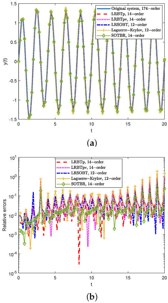
Figure 1.
Transient responses and relative errors of the ROMs in Example 1. (a) Transient responses. (b) Relative errors.

Table 1.
Computational information of Example 1.
Table 2.
Relative errors at different time t for Example 1.
According to the results, it is evident that all the ROMs effectively approximated the transient responses of the original system. Figure 1b indicates that our methods achieved better performance than the Laguerre–Krylov method. In addition, in Table 1, we can see that Algorithm 3 (LRSOBT method) was the most efficient in generating the reduced second-order TDS, and the simulation time of the ROM obtained using Algorithm 3 (LRSOBT method) was the shortest. Table 2 shows the relative errors at different times t with acceptable accuracy, indicating the effectiveness of the proposed method. The proposed algorithms achieved acceptable accuracy and computational efficiency.
5.2. Example 2
Consider a second-order TDS (1) with the constant matrices ,
and . The external force B is a vector with zeros everywhere, except the last entry, which is one, and we set . We chose the exact parameters for this example, with , , , , , and . For details, please refer to [19].
The proposed algorithms were executed with and the Laguerre expansion terms . For our methods and the Laguerre–Krylov method, the Laguerre parameter was set to . The adaptive order r of the ROMs constructed through our algorithms was 12, and we set the order of the ROMs generated through the Laguerre–Krylov method and SOTBR method to 12 and 35, respectively, according to [22]. Given the input , the performances of the original second-order TDS and the ROMs in the time domain are presented in Figure 2. The time domain responses of the original second-order TDS and the five ROMs are shown in Figure 2a. The corresponding absolute errors of all ROMs are displayed in Figure 2b. Table 3 reports the computational times for solving all systems and generating the ROMs of our methods and the two reference methods. Table 4 shows the absolute errors at different times t.
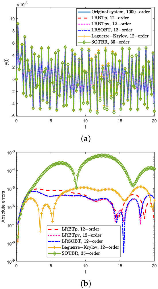
Figure 2.
Transient responses and absolute errors of the ROMs in Example 2. (a) Transient responses. (b) Absolute errors.
Table 3.
Computational information of Example 2.
Table 4.
Absolute errors at different times t for Example 2.
According to the results, it is evident that all the ROMs effectively approximated the transient response of the original second-order TDS. Figure 2b shows that our proposed algorithms and the Laguerre–Krylov method performed better and obtained smaller absolute errors than the SOTBR method. In addition, Table 3 demonstrates that the proposed algorithms achieved acceptable accuracy. In particular, the LRSOBT method demonstrated the best efficiency for generating the reduced second-order TDS and simulation compared with the first-order approaches and the two reference approaches. Table 4 shows the absolute errors at different times t with relatively high accuracy, indicating the effectiveness of the proposed method.
It is worth mentioning that the choice of the Laguerre parameter has a significant impact on the accuracy and stability of Laguerre-based MOR algorithms when constructing ROMs. Although [31] provided relevant results for LTI systems, additional research is required to determine the optimal Laguerre parameter for more general scenarios. In addition, although we did not encounter instability in the ROMs obtained using the proposed techniques in the above experiments, preserving stability cannot be guaranteed in general.
6. Conclusions
Throughout this research, our primary focus is on discussing MOR approaches for second-order time-delay systems, specifically emphasizing low-rank Gramian approximations. Two paths, the first-order method and the second-order method, for constructing ROMs are presented, and three structure-preserving MOR algorithms utilizing the Laguerre functions are showcased. The main objective is to obtain the low-rank decomposition of the time-delay controllability and observability Gramians in the frequency domain, which can be computed efficiently using recurrence formulas based on the Laguerre expansions, making the approach highly efficient and flexible. Utilizing the low-rank time-delay Gramians, a collection of structure-preserving MOR algorithms is proposed by combining the ideas of the LRSRM. Finally, we showcase the efficacy of the proposed method by providing numerical examples, highlighting its superior performance compared to existing reduction techniques.
Author Contributions
Methodology, M.T., Z.-H.X. and U.Z.; Writing—original draft, M.T.; Writing—review & editing, Z.-H.X. and U.Z.; Supervision, Z.-H.X. and U.Z.; Project administration, Z.-H.X. All authors have read and agreed to the published version of the manuscript.
Funding
This work was supported by the National Natural Science Foundation of China (NSFC) under grants 62273059 and 62350410484, and in part by the High-End Foreign Expert Programs No. G2023027005L, granted by the State Administration of Foreign Experts Affairs (SAFEA).
Data Availability Statement
The data generated and analyzed in this study are available from the corresponding author upon request.
Conflicts of Interest
The authors declare no conflicts of interest.
References
- Erneux, T. Applied Delay Differential Equations; Springer Science & Business Media: Berlin/Heidelberg, Germany, 2009; Volume 3. [Google Scholar]
- Kolmanovskii, V.; Myshkis, A. Applied Theory of Functional Differential Equations; Springer Science & Business Media: Berlin/Heidelberg, Germany, 2012; Volume 85. [Google Scholar]
- Altintas, Y.; Ber, A. Manufacturing automation: Metal cutting mechanics, machine tool vibrations, and CNC design. Appl. Mech. Rev. 2001, 54, B84. [Google Scholar] [CrossRef]
- Michiels, W.; Niculescu, S.I. Stability and Stabilization of Time-Delay Systems: An Eigenvalue-Based Approach; SIAM: New Delhi, India, 2007. [Google Scholar]
- Gu, K.; Chen, J.; Kharitonov, V.L. Stability of Time-Delay Systems; Springer Science & Business Media: Berlin/Heidelberg, Germany, 2003. [Google Scholar]
- Hamadi, M.A.; Jbilou, K.; Ratnani, A. A model reduction method in large scale dynamical systems using an extended-rational block Arnoldi method. J. Appl. Math. Comput. 2022, 68, 271–293. [Google Scholar] [CrossRef]
- Wang, X.; Wang, Q.; Zhang, Z.; Chen, Q.; Wong, N. Balanced truncation for time-delay systems via approximate Gramians. In Proceedings of the 16th Asia and South Pacific Design Automation Conference (ASP-DAC 2011), Yokohama, Japan, 25–28 January 2011; IEEE: Piscataway, NJ, USA, 2011; pp. 55–60. [Google Scholar]
- Huang, L.; Zhao, H.; Sun, T. An iterative proper orthogonal decomposition method for a parabolic optimal control problem. J. Appl. Math. Comput. 2024, 70, 47–72. [Google Scholar] [CrossRef]
- Michiels, W.; Jarlebring, E.; Meerbergen, K. Krylov-based model order reduction of time-delay systems. SIAM J. Matrix Anal. Appl. 2011, 32, 1399–1421. [Google Scholar] [CrossRef]
- Duff, I.P.; Vuillemin, P.; Poussot-Vassal, C.; Seren, C.; Briat, C. Approximation of stability regions for large-scale time-delay systems using model reduction techniques. In Proceedings of the 2015 European Control Conference (ECC), Linz, Austria, 15–17 July 2015; IEEE: Piscataway, NJ, USA, 2015; pp. 356–361. [Google Scholar]
- Samuel, E.R.; Knockaert, L.; Dhaene, T. Model order reduction of time-delay systems using a Laguerre expansion technique. IEEE Trans. Circuits Syst. I Regul. Pap. 2014, 61, 1815–1823. [Google Scholar] [CrossRef]
- Wang, X.L.; Jiang, Y.L. Time domain model reduction of time-delay systems via orthogonal polynomial expansions. Appl. Math. Comput. 2020, 369, 124816. [Google Scholar] [CrossRef]
- Wang, X.L.; Jiang, Y.L. An efficient hybrid reduction method for time-delay systems using Hermite expansions. Int. J. Control 2019, 92, 1033–1043. [Google Scholar] [CrossRef]
- Rasekh, E.; Dounavis, A. Multiorder Arnoldi approach for model order reduction of PEEC models with retardation. IEEE Trans. Components, Packag. Manuf. Technol. 2012, 2, 1629–1636. [Google Scholar] [CrossRef]
- Besselink, B.; Chaillet, A.; van de Wouw, N. Model reduction for linear delay systems using a delay-independent balanced truncation approach. In Proceedings of the 2017 IEEE 56th Annual Conference on Decision and Control (CDC), Melbourne, VIC, Australia, 12–15 December 2017; IEEE: Piscataway, NJ, USA, 2017; pp. 3793–3798. [Google Scholar]
- Jarlebring, E.; Damm, T.; Michiels, W. Model reduction of time-delay systems using position balancing and delay Lyapunov equations. Math. Control Signals Syst. 2013, 25, 147–166. [Google Scholar] [CrossRef]
- Qiu, Z.Y.; Jiang, Y.L. ε-Embedding model reduction method for time-delay differential algebra systems. Circuits Syst. Signal Process. 2020, 39, 5390–5405. [Google Scholar] [CrossRef]
- Naderi Lordejani, S.; Besselink, B.; Chaillet, A.; van de Wouw, N. On extended model order reduction for linear time delay systems. In Model Reduction of Complex Dynamical Systems; Springer: Berlin/Heidelberg, Germany, 2021; pp. 191–215. [Google Scholar]
- Saadvandi, M.; Meerbergen, K.; Jarlebring, E. On dominant poles and model reduction of second order time-delay systems. Appl. Numer. Math. 2012, 62, 21–34. [Google Scholar] [CrossRef]
- Wang, X.L.; Jiang, Y.L.; Kong, X. Laguerre functions approximation for model reduction of second order time-delay systems. J. Frankl. Inst. 2016, 353, 3560–3577. [Google Scholar] [CrossRef]
- Xiao, Z.H.; Jiang, Y.L. Multi-order Arnoldi-based model order reduction of second-order time-delay systems. Int. J. Syst. Sci. 2016, 47, 2925–2934. [Google Scholar] [CrossRef]
- Jiang, Y.L.; Qiu, Z.Y.; Yang, P. Structure preserving model reduction of second-order time-delay systems via approximate Gramians. IET Circuits Devices Syst. 2020, 14, 130–136. [Google Scholar] [CrossRef]
- Gugercin, S.; Antoulas, A.C. A survey of model reduction by balanced truncation and some new results. Int. J. Control 2004, 77, 748–766. [Google Scholar] [CrossRef]
- Meyer, D.G.; Srinivasan, S. Balancing and model reduction for second-order form linear systems. IEEE Trans. Autom. Control 1996, 41, 1632–1644. [Google Scholar] [CrossRef]
- Benner, P.; Kürschner, P.; Saak, J. Frequency-limited balanced truncation with low-rank approximations. SIAM J. Sci. Comput. 2016, 38, A471–A499. [Google Scholar] [CrossRef]
- Xiao, Z.H.; Song, Q.Y.; Jiang, Y.L.; Qi, Z.Z. Model order reduction of linear and bilinear systems via low-rank Gramian approximation. Appl. Math. Model. 2022, 106, 100–113. [Google Scholar] [CrossRef]
- Wang, X.; Zhang, Z.; Wang, Q.; Wong, N. Gramian-based model order reduction of parameterized time-delay systems. Int. J. Circuit Theory Appl. 2014, 42, 687–706. [Google Scholar] [CrossRef]
- Du, X.; Liu, F.; Zhu, X.; Chao, W. Finite frequency approaches to H∞ model reduction for continuous-time state delayed systems. In Proceedings of the 2012 24th Chinese Control and Decision Conference (CCDC), Taiyuan, China, 23–25 May 2012; IEEE: Piscataway, NJ, USA, 2012; pp. 470–475. [Google Scholar]
- Penzl, T. Algorithms for model reduction of large dynamical systems. Linear Algebra Its Appl. 2006, 415, 322–343. [Google Scholar] [CrossRef]
- Reis, T.; Stykel, T. Balanced truncation model reduction of second-order systems. Math. Comput. Model. Dyn. Syst. 2008, 14, 391–406. [Google Scholar] [CrossRef]
- Knockaert, L.; De Zutter, D. Laguerre-SVD reduced-order modeling. IEEE Trans. Microw. Theory Tech. 2000, 48, 1469–1475. [Google Scholar] [CrossRef]
- Zang, Z.; Cantoni, A.; Teo, K.L. Continuous-time envelope-constrained filter design via Laguerre filters and H∞ optimization methods. IEEE Trans. Signal Process. 1998, 46, 2601–2610. [Google Scholar] [CrossRef]
- Szeg<i>ö</i>, G. Orthogonal Polynomials; American Mathematical Society: New York, NY, USA, 1939. [Google Scholar]
- Rassias, T.M.; Srivastava, H. Some general families of generating functions for the Laguerre polynomials. J. Math. Anal. Appl. 1993, 174, 528–538. [Google Scholar] [CrossRef][Green Version]
- Xiao, Z.H.; Jiang, Y.L.; Qi, Z.Z. Structure preserving balanced proper orthogonal decomposition for second-order form systems via shifted Legendre polynomials. IET Control Theory Appl. 2019, 13, 1155–1165. [Google Scholar] [CrossRef]
- Dai, L.; Xiao, Z.H.; Zhang, R.Z.; Jiang, Y.L. Laguerre-Gramian-based structure-preserving model order reduction for second-order form systems. Trans. Inst. Meas. Control 2022, 44, 1113–1124. [Google Scholar] [CrossRef]
- Li, J.R.; White, J. Low rank solution of Lyapunov equations. SIAM J. Matrix Anal. Appl. 2002, 24, 260–280. [Google Scholar] [CrossRef]
- Breiten, T. Structure-preserving model reduction for integro-differential equations. SIAM J. Control Optim. 2016, 54, 2992–3015. [Google Scholar] [CrossRef]
- Benner, P.; Mehrmann, V.; Sorensen, D.C. Dimension Reduction of Large-Scale Systems; Springer: Berlin/Heidelberg, Germany, 2005; Volume 45. [Google Scholar]
Disclaimer/Publisher’s Note: The statements, opinions and data contained in all publications are solely those of the individual author(s) and contributor(s) and not of MDPI and/or the editor(s). MDPI and/or the editor(s) disclaim responsibility for any injury to people or property resulting from any ideas, methods, instructions or products referred to in the content. |
© 2025 by the authors. Licensee MDPI, Basel, Switzerland. This article is an open access article distributed under the terms and conditions of the Creative Commons Attribution (CC BY) license (https://creativecommons.org/licenses/by/4.0/).