Optimization of Autoencoders for Speckle Reduction in SAR Imagery Through Variance Analysis and Quantitative Evaluation

Abstract

Speckle reduction in Synthetic Aperture Radar (SAR) images is a crucial challenge for effective image analysis and interpretation in remote sensing applications. This study proposes a novel deep learning-based approach using autoencoder architectures for SAR image despeckling, incorporating analysis of variance (ANOVA) for hyperparameter optimization. The research addresses significant gaps in existing methods, such as the lack of rigorous model evaluation and the absence of systematic optimization techniques for deep learning models in SAR image processing. The methodology involves training 240 autoencoder models on real-world SAR data, with performance metrics evaluated using Mean Squared Error (MSE), Structural Similarity Index (SSIM), Peak Signal-to-Noise Ratio (PSNR), and Equivalent Number of Looks (ENL). By employing Pareto frontier optimization, the study identifies models that effectively balance denoising performance with the preservation of image fidelity. The results demonstrate substantial improvements in speckle reduction and image quality, validating the effectiveness of the proposed approach. This work advances the application of deep learning in SAR image denoising, offering a comprehensive framework for model evaluation and optimization.

1. Introduction

Synthetic Aperture Radar (SAR) is an imaging technique that uses active sensors to create high-resolution images of the Earth’s surface. SAR satellites send microwave signals to the target area, record and process the reflected signal to generate images [1]. SAR images suffer from speckle, a spatially correlated, signal-dependent noise that degrades quality and complicates processing [2]. Speckle originates from the coherent nature of SAR systems, hiding scene details [3] and making analysis challenging. Traditional denoising methods are often ineffective [4]. The nature and characteristics of speckle in SAR images have been modeled. This model includes a multiplicative component of speckle in the amplitude and an additive component in the phase. To eliminate the multiplicative component, various image processing and filtering techniques are employed, such as Spatial Filtering (including mean filtering, median filtering, and Lee filtering) [3], Frequency Domain Filtering (utilizing Fourier transforms and corresponding filtering), Statistics-Based Filtering (using local or global statistics, such as the Frost filter), SAR Despeckling and Restoration (involving multiplicative component decomposition), Wavelet-Based Filtering, and Non-Local Filtering [5]. Similarly, for the removal of the additive component, which is considered a more complex challenge than treating the multiplicative component in the amplitude, some of the strategies and techniques used to address or reduce this component include Spatial Filtering in the Phase (using spatial domain mean or median filters) [6], SAR Interferometry (InSAR), Statistical Methods and Advanced Models (including Kalman filtering and methods based on random field theory), Wavelet-Based Phase Filtering, Joint Phase Processing (SAR interferometry), and Constant Amplitude Phase Techniques. Finally, in many cases, a combination of multiple techniques is applied to achieve better results [7].

Speckle in SAR images has been addressed through various techniques, including spatial filtering, frequency domain filtering, statistics-based filtering, SAR despeckling and restoration, wavelet-based filtering, and non-local filtering. Additionally, methods for dealing with the more complex additive component in the phase involve spatial filtering, SAR interferometry, statistical methods, advanced models, wavelet-based phase filtering, joint phase processing, and constant amplitude phase techniques. Often, a combination of these techniques is used for optimal results [7]. Deep learning approaches have emerged as a solution for despeckling SAR images, benefiting from their ability to learn complex features, handle noisy data, and improve image quality. These models contribute to enhanced classification, segmentation, and object detection, making them valuable in various SAR image analysis contexts [8,9].

It is essential to highlight that with deep learning, it is possible to reduce time and effort by automating the extraction of relevant features from SAR images, simplifying data preprocessing. Furthermore, the scalability of these models and their ability to leverage specialized hardware and software makes them a powerful option for processing large volumes of SAR imagery, facilitating advances in the interpretation and analysis of these images for different applications [10].

Deep learning-based SAR image despeckling uses algorithms like U-Net and deSpeckNet, showing promise in reducing speckle [11]. These and other techniques utilize evaluation metrics like PSNR (Peak Signal-to-Noise Ratio) and SSIM (Structural Similarity Index) to compare despeckled images to originals [12]. Based on the results obtained, it was found that when applying deep learning techniques, it is possible to mitigate speckle but it can introduce artifacts along feature boundaries [13].

In light of all that has been previously discussed and considering the significant advantages of deep learning in SAR image processing, there is still a justification for new proposals where these algorithms can substantially contribute to enhancing the results achieved and documented in the scientific literature. As an active area of research in recent decades, the emergence of the DL paradigm has established a clear division between all methods: traditional despeckling techniques like [14], and the ones based on DL, like [15,16,17,18], among others.

The availability of diverse and high-quality datasets plays a critical role in effectively training deep learning models aimed at reducing smearing in SAR images [12]. A complete dataset allows the model to recognize the complexities and variations present in SAR images, facilitating reliable learning and effective noise reduction. Likewise, it allows covering different terrains and climatic conditions of the study surfaces, guaranteeing that the model learns to recognize multiple scenarios and improves its generalization capacity. This process helps address the challenges associated with SAR imagery speckle by allowing the model to recognize the patterns and characteristics of this noise type, leading to more effective speckle reduction strategies [19].

In the pursuit of identifying the best autoencoder architecture, an experiment was conducted, encompassing the training of 240 autoencoders on a dataset comprising 1500 training images and 100 validation images. The dataset was designed in [20] and each autoencoder architecture was evaluated using the ground truth defined in the validation set.

In this paper, we propose a new methodology and results derived from applying analysis of variance (ANOVA) to determine the most appropriate hyperparameters for an autoencoder model aimed at reducing the speckle in SAR images. When training deep learning models such as the autoencoder used in this study, researchers and developers used to modify the hyperparameters, seeking for optimal solutions with a heuristic approach, trial-and-error tests, without a systematic path to determine the best configuration of these parameters. In our methodology, ANOVA emerges as an organized and systematic methodology to determine the optimal parameters for the model. The methodology involves the evaluation of performance metrics, Mean Squared Error (MSE), Structural Similarity Index (SSIM), Maximum Signal-to-Noise Ratio (PSNR), and Equivalent Number of Looks (ENL), acquired from training a set of 240 different autoencoder models using various hyperparameter configurations. Our results delve into analyzing these metrics to find optimal trade-offs and identify the settings that best mitigate speckle while preserving SAR image quality.

This paper is organized as follows. In Section 2, the dataset is described along with the autoencoder model structure. In Section 3, the models are trained, a description of the different configurations of the hyperparameters is presented, and the ANOVA methodology is described. In Section 4, the main findings and results are shown. In Section 5, the discussion of the results is carried out, with an emphasis on the novelty of the research. Finally, in Section 6, some relevant conclusions are outlined.

2. Materials and Methods

In this section, the materials used and the methodologies employed on SAR image despeckling using convolutional denoising autoencoder (CDAE) techniques are presented. The challenges from SAR image despeckling and the scarcity of ground-truth datasets have motivated innovative approaches aimed at addressing these obstacles. The initial subsection delves into the dataset used, coming from SAR images of Toronto, ON, Canada in 2022, highlighting the creation of a ground-truth reference image for evaluation. The next subsection explores the application of autoencoder as a technique for SAR image despeckling, emphasizing its potential to address the complexities associated with despeckle. Finally, an exploration of ANOVA statistical analysis and its role in optimizing hyperparameter selection for autoencoder-based SAR image despeckling models is covered.

2.1. The Dataset

The speckle in SAR images refers to the grainy or granular interference pattern that appears as bright and dark randomly allocated points throughout the image. It is a multiplicative noise related to the coherent nature of SAR imaging, where electromagnetic waves reflected from different scattering centers interfere with each other, creating constructive and destructive patterns that leads to variations in pixel intensities. The speckle presence in an image can alter some details in SAR imagery, making it challenging for image interpretation and analysis [7]. An ideal filter should remove the speckle while preserving spatial information without introducing artifacts [21].

A SAR image Y can be mathematically expressed as:

$$Y=f(X,N)=X·N,$$

(1)

where X is the corresponding noise-free image and N is the speckle. The speckle has a Gamma distribution [22,23]. This distribution is given by Equation (2):

$$p\left(N\right)={\displaystyle \frac{1}{\Gamma \left(L\right)}}{N}^L{e}^{-NL},$$

(2)

where L is the number of looks (ENL) of the SAR image.

The dataset used consists of actual Synthetic Aperture Radar (SAR) imagery obtained from the ASF Datasearch Vertex. The specific dataset used is Sentinel 1A imagery of the region of Toronto in 2022. The images were acquired in intensity mode level “L1 Detected High-Res Dual-Pol (GRD-HD)” from 24 August to 22 December, with a revisiting period of 12 days. The images were obtained using the C band at 5.4 GHz with a resolution of 10 m and VV polarization at a height of 693 km from Ecuador.

To create a ground truth reference image for evaluation, a multitemporal fusion technique was applied. A reference image from 5 September was selected, and four additional images were registered and averaged with respect to it. This process was repeated with nine more images, resulting in a total of ten images being averaged. The Equivalent Number of Looks (ENL) was calculated for the three resulting images, indicating the level of noise reduction achieved. A mean of 10 samples was used according to [20].

Figure 1 presents a reference image of the SAR dataset utilized in the paper, showcasing the ground-truth image and ground-truth image zoom in the first column and their corresponding noised counterparts in the second column. This illustrative image serves to highlight the impact of speckle on SAR images and the necessity of effective despeckle techniques for preserving features in different applications.

The dataset also includes image clipping, where specific regions of interest were selected for evaluation. The dataset was designed to overcome the limitations of using synthetic images with speckle models by providing more realistic SAR data for testing despeckling filters.

2.2. Convolutional Denoising Autoencoder (CDAE) for SAR Image Despeckling

Despeckling an image is an essential preprocessing step for eliminating undesired patterns and having noiseless images for any future postprocessing task, such as classification, object detection, segmentation, among others.

SAR image despeckling faces several challenges due to the nature of speckle and the limited availability of speckle-free SAR images [19,24]. Additionally, removing speckle while preserving image details such as edges and textures is a challenging task [19]. In recent years, various approaches have been proposed to address these challenges, including traditional filters, statistical models, and machine learning-based methods. Among these approaches, deep learning-based methods have shown promising results in SAR image despeckling, with autoencoder being one of the most effective methods [19]. SAR image despeckling is important for accurate image analysis in different applications. The removal of speckle can improve the quality of SAR images, making it easier to extract useful information and perform subsequent analyses [24]. Deep learning-based approaches, such as CDAE, have shown potential in addressing the challenges associated with SAR image despeckling [25]. The use of these methods can lead to improved accuracy and efficiency in SAR image analysis, making it an important area of research [26].

Convolutional Neural Networks (CNNs) are a type of neural network commonly used for image processing tasks, including image classification, segmentation, and denoising [27]. CNN consist of multiple layers, including convolutional layers that apply filters to the input image, pooling layers that downsample the output, and fully connected layers that perform classification tasks [28]. The ability of CNN to learn complex image features has made them a popular choice for SAR image processing tasks, including despeckling. Denoising Autoencoders (DAEs) are a type of neural network that can learn to remove noise from input data. This method consist of two parts: an encoder that maps the input data to a lower-dimensional representation, and a decoder that maps the lower-dimensional representation back to the original input. By training the network on noisy input data and clean output data, the network can learn to remove noise from new input data [29].

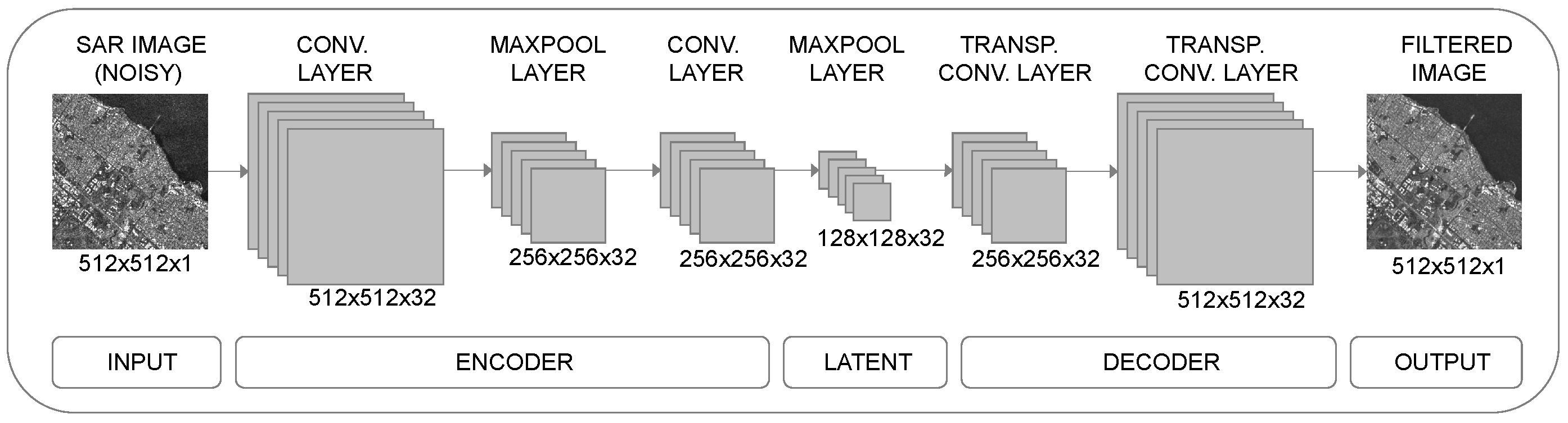
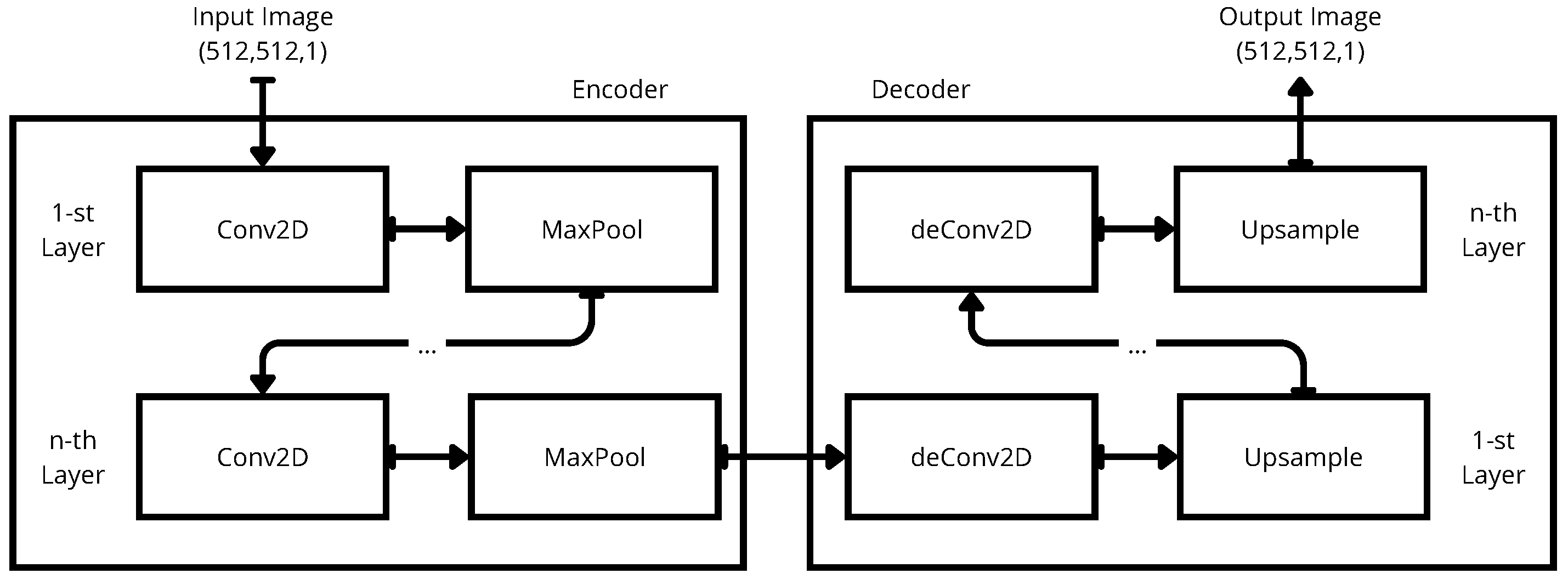
Convolutional Denoising Autoencoder (CDAE) is a type of DAE that uses convolutional layers for image processing tasks [19]. The CDAE architecture consists of an encoder that applies a series of convolutional and pooling layers to the input image, followed by a decoder that applies a series of deconvolutional and upsampling layers to reconstruct the clean image. By training the network on noisy input data and clean output data, the network can learn to remove speckle from new input SAR images [12]. The use of CDAE for SAR image despeckling has shown promising results, with improved image quality and preservation of important features compared to traditional filtering methods (see Figure 2).

The study involves the training of various autoencoder structures, systematically varying the depth and the number of convolutional layers to identify the optimal architecture that yields the most effective reduction of speckle. Exploring a range of network depths and convolutional layer configurations enables the determination of the most suitable CDAE structure for the SAR image despeckling task. This approach aims to achieve superior despeckling performance while preserving essential image features critical for accurate SAR image analysis. The selected CDAE architecture effectively balances noise reduction and feature preservation in actual SAR images, enhancing the interpretability and utility of the despeckled images for downstream analysis and applications, with the results presented in [30].

2.3. ANOVA and Its Application in Machine Learning

Analysis of variance (ANOVA) is a statistical technique used in various fields to determine whether there are significant differences between groups or not, and to identify factors that may contribute to these differences [31]. Machine learning (ML) is used to analyze the impact of different hyperparameters on the performance of a model. It allows us to identify and optimize the most important hyperparameters to improve the model’s accuracy [32]. Hyperparameters are variables that are set before the model is trained. Additionally, ANOVA can provide insights into the relationships between hyperparameters and their impact on the model’s performance, allowing hyperparameter tuning based on statistical criteria [31].

In the context of speckle denoising autoencoder models, ANOVA can be used to identify the most important hyperparameters for optimizing the model’s performance [33]. The hyperparameter list includes factors such as the number of layers, the learning rate, and the batch size. By analyzing the impact of these hyperparameters on the model’s accuracy, ANOVA can help to optimize the model for better performance while reducing overfitting [33]. ANOVA can also be used to compare the performance of different models and identify the most effective approach for speckle denoising [34]. Our novel approach is the use of ANOVA as a powerful tool for hyperparameter optimization in machine learning to improve the accuracy and efficiency of despeckling autoencoder models.

3. Experimental Methodology

This section presents the training process of 240 autoencoder models for speckle reduction in SAR images. The dataset was partitioned into training, testing, and validation sets, enabling an assessment of the model’s generalization ability. Various architectures were explored to strike a balance between speckle reduction and preservation of essential image features, highlighting challenges in their selection and approaches for efficient tuning. Statistical analyses, evaluation metrics, and comparative studies are discussed to comprehend the performance of diverse autoencoder architectures.

3.1. Autoencoder Model Training

The comparison procedure involved an evaluation of 240 distinct autoencoder models trained with a set of 1500 SAR images. The dataset was divided, with 85% of the images for training and the remaining 15% reserved for testing, ensuring an assessment of the model performance. Moreover, to gauge the generalization capability of the trained models, an additional set of 100 SAR images was set aside for validation. This approach allowed a comprehensive assessment of how effectively the trained models could generalize to unseen SAR data, underscoring the robustness of the selected architecture and hyperparameter configurations.

The training of the 240 autoencoder models was systematically conducted, encompassing all possible combinations of 6 hyperparameters: i—the number of convolutional layers, ii—the number of filters per layer, iii—the activation function, iv—batch size, v—loss function, and vi—learning rate, leveraging the comprehensive dataset comprising 1500 images affected by speckle and an additional 1500 noise-free images as ground-truth. The training process was performed in two stages. First, the models were trained using the ground-truth images as input and output, allowing the models to grasp the characteristics and patterns of the SAR images. Finally, the training was conducted using the noisy images as inputs and the corresponding ground-truth images as desired outputs.

In order to obtain an effective method to despeckle SAR images, we used different autoencoder architectures by varying their related hyperparameters. Figure 3 shows the basic autoencoder architecture used.

3.2. Hyperparameters in Autoencoder Models

Hyperparameters are parameters set before training an autoencoder model that determine the model’s architecture and training process. These parameters include the number of layers, the number of neurons in each layer, the learning rate, the regularization parameter, among others [35]. The choice of hyperparameters can significantly affect the performance of the model. For instance, in the case of a denoising autoencoder, the level of noise added to the input data and the strength of the denoising process are hyperparameters that can impact the model’s ability to remove noise and reconstruct the original data [29].

The importance of hyperparameters in autoencoder models lies in their ability to influence the performance and generalization capacity of the model. Selecting appropriate hyperparameters can lead to better model accuracy and faster convergence. However, the hyperparameter selection process can be challenging, and trial-and-error methods can be time-consuming and computationally expensive [35]. One approach to address this challenge is to use statistical methods such as ANOVA to determine the most important hyperparameters and their optimal values. This approach can help reduce the search space and improve the efficiency of training [36].

Each of the 240 trained autoencoder models (

Table 1. Hyperparameter values for trained models.

Hyperparameter	Values
Convolutional Layers	[4, 6]
Filters	[32, 64]
Activation Functions	[‘relu’, ‘elu’]
Batch Size	[2, 4, 8, 16, 32]
Loss	[‘mse’, ‘bce’]
Learning Rate	[0.001, 0.005, 0.01]

) underwent an evaluation to assess their proficiency in reducing speckles while preserving features and details within SAR images. The evaluation process employed various performance metrics, including structural similarity index (SSIM) and peak signal-to-noise ratio (PSNR), to quantitatively measure the fidelity of noise-free images. This evaluation framework aimed to identify the optimal configuration of autoencoder models, balancing speckle reduction.

The comparison is conducted by examining the variation of different hyperparameters during the training of the autoencoders to determine the optimal combination that achieves maximum speckle reduction. The research aims to identify the configuration that not only minimizes noise but also enhances the model’s ability to reconstruct the original image accurately. This comparison allows for the exploration of the impact of each hyperparameter on the performance and generalization ability of the autoencoder model, providing valuable insights into the interplay between hyperparameter settings and the efficacy of speckle reduction in SAR imagery.

3.3. Understanding Ablation

Ablation is a crucial tool in neural network research, allowing the critical components of the network to be identified and its performance to be improved. This technique helps understand how the network processes information and what features are crucial for making accurate predictions. By gaining insight into the inner workings of the network, adjustments can be made to improve its overall performance. Ablation also helps identify unnecessary functions, leading to more efficient and optimized networks. This process involves selectively removing or disabling specific components of the neural network and observing the resulting changes in performance [37].

The process proposed in this paper by using ANOVA is a much deeper and complete analysis than the ablation process, since it addresses the whole impact of all the hyperparameters and the modifications performed on the model, while the ablation consists of eliminating or altering some parts of the model to measure its individual effects.

3.4. ANOVA Methodology

To begin a comparison of the 240 autoencoder models, an analysis of variance was initiated, examining the performance variations among the different filtering architectures. The analysis commenced with the formulation of the following hypotheses. The null hypothesis ($H_0$) stipulated that the average performance of all filtering architectures was not different, while the alternative hypothesis ($H_1$) proposed the existence of at least one filtering architecture whose performance differed from the rest. This statistical approach allowed for a examination of the efficacy of the autoencoder models, shedding light on the impact of different filtering strategies on the denoising capabilities.

In statistics, the letter p is used to represent the p-value, which is a measure of evidence against a null hypothesis in a statistical analysis. The p-value represents the probability of obtaining a result as extreme as, or more extreme than, the observed data, assuming that the null hypothesis is true. If it is less than a predefined threshold, the results are considered statistically significant, suggesting that the null hypothesis is unlikely and should be rejected in favor of the alternative hypothesis.

Mathematically, the p-value is commonly represented according to Equation (3):

$$p=P(X\ge x\mid H_0),$$

(3)

where X is a random variable representing the test statistic, x is the observed value of the test statistic, and $H_0$ is the null hypothesis. The p-value is interpreted as the probability of obtaining a result as extreme as, or more extreme than, the observed data, assuming that the null hypothesis is true.

The subsequent selection process focused on identifying the subset of models residing on the Pareto frontier. The objective was to find the models that exhibited the most favorable performance across multiple evaluation metrics. The initial strategy entailed identifying the models characterized by the highest average performance across all the performance metrics. This approach sought to pinpoint the models that demonstrated consistent and robust performance, highlighting their potential as promising candidates for further in-depth analysis and deployment in practical applications. By prioritizing the selection of models based on their holistic performance profiles, the aim is to ascertain the most reliable and high-performing configurations.

The Pareto frontier represents the set of all optimal solutions where no single objective can be improved without degrading at least one other objective. This fundamental concept helped in identifying the trade-off between competing objectives and provided a comprehensive understanding of the performance landscape of the various autoencoder architectures under consideration.

3.5. Metrics for SAR Images

In order to measure the quality of an image and the presence of speckle on it, a comparison with respect to another one, there are several metrics widely used in the literature.

3.5.1. Mean Squared Error (MSE)

The MSE is a metric calculated of one complete image with respect to another one. Is an operation that is performed pixel by pixel, by accumulating the error of the squared difference between them. The MSE is calculated according to Equation (4).

$$MSE={\displaystyle \frac{1}{N}}\sum _{i=0}^{m-1}\sum _{j=0}^{n-1}{(Y(i,j)-Z(i,j))}^2,$$

(4)

where $Y(i,j)$ and $Z(i,j)$ are the $(i,j)-th$ pixels of images Y and Z, respectively, m is the number of rows, n is the number of columns and $N=m\times n$.

3.5.2. Structural Similarity Index (SSIM)

The SSIM is a metric used to assess the similarity between two images. It measures the similarity in terms of luminance, contrast, and structure. The SSIM index is calculated using Equation (5):

$$SSIM(x,y)={\displaystyle \frac{(2{\mu }_x{\mu }_y+c_1)·(2{\sigma }_{xy}+c_2)}{({\mu }_x^2+{\mu }_y^2+c_1)·({\sigma }_x^2+{\sigma }_y^2+c_2)}},$$

(5)

where ${\mu }_x$ and ${\mu }_y$ are the average pixel values of images x and y, respectively, ${\sigma }_x$ and ${\sigma }_y$ are the standard deviations of x and y, ${\sigma }_{xy}$ is the covariance between x and y, and $c_1$ and $c_2$ are constants to stabilize the division.

3.5.3. Peak Signal-to-Noise Ratio (PSNR)

The PSNR is a metric used to measure the quality of reconstruction of lossy compression codecs. It is defined as the ratio between the maximum possible power of a signal and the power of corrupting noise that affects the fidelity of its representation. The PSNR is calculated using Equation (6):

$$PSNR=10·{log}_{10}\left({\displaystyle \frac{MA{X}^2}{MSE}}\right),$$

(6)

where $MAX$ is the maximum possible pixel value of the images and $MSE$ is the mean squared error between the two images.

3.5.4. Equivalent Number of Looks (ENL)

The ENL is calculated in a homogeneous region of 20 × 20 pixels of the image. A value of $ENL=1$ is the worst scenario; a higher value means the most homogeneous (filtered) region is the region measured. It is calculated according to Equation (7).

$$ENL={\displaystyle \frac{{\mu }^2}{{\sigma }^2}},$$

(7)

where $\mu$ is the mean intensity and $\sigma$ is the standard deviation of all the pixels in the selected homogeneous region.

According to these measurements, it is possible to compare the performance of a despeckling process against another one proposed by other authors.

Evaluation metrics play a crucial role in assessing speckle reduction in SAR images. These metrics, including MSE, SSIM, PSNR and ENL, offer valuable insights into image quality. A lower MSE value closer to 0 signifies superior despeckling performance, indicating minimal error between the filtered and original images. SSIM, with values approaching 1, measures the similarity in luminance, contrast, and structure, highlighting high resemblance between the denoised and pristine images. Additionally, higher PSNR values denote better reconstruction quality by quantifying the ratio between signal power and noise. Similarly, ENL, reflecting higher values, signifies greater homogeneity in the filtered region. These metrics collectively provide comprehensive assessments, emphasizing fidelity to the original image, similarity, and noise reduction, crucial for effective SAR image analysis and interpretation.

3.6. Proposed Method to Select the Best Model

In order to select a model $M^{\ast }$ among the subset of n optimal architectures, a heuristic methodology, based on a systematic ranking of the performance metrics, was developed (Algorithm 1).

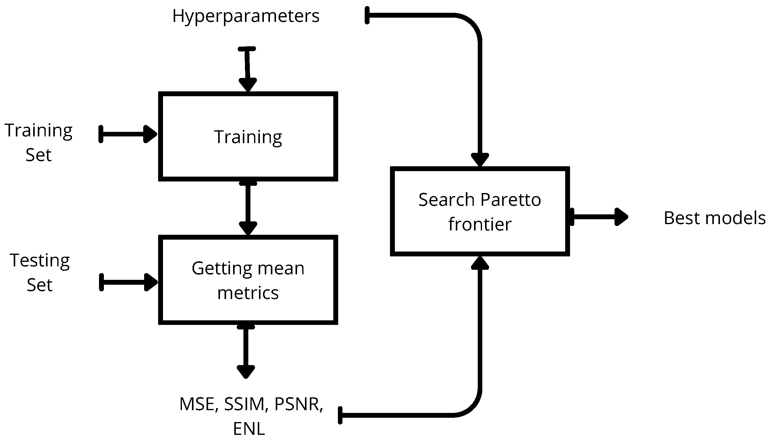
In summary, the proposed methodology for systematically and efficiently tuning hyperparameters, as well as selecting the optimal model, is illustrated in Figure 4. The process begins with the training and test datasets as inputs. The model is then trained and validated using the specified metrics, which include both mean and standard deviation. Ultimately, the Pareto frontier analysis, combined with score ranking, facilitates the identification of the most suitable model.

Algorithm 1 Proposed algorithm to select the best model $M^{\ast }$.

Input: $M=\{Models\in \mathrm{Pareto} \mathrm{frontier}\}$//M is the set of best models $\phi =\{MSE,SSIM,PSNR,ENL\}$//φ is the set of metrics $w_{\phi }\in R^4,0\le w_{\phi }^i\le 1,{\sum }_i{w}_{\phi }^i=1$//$w_{\phi }$ is the set of metric weights Output: $M^{\ast }$ as the best model among the set of all models M for each element of M do     for each element of $\phi$ do           $\overline{\phi }\left(M\right)\leftarrow \mathrm{avg}\left(\phi \left(M\right)\right)$ //The mean value of the metrics           $D_{\overline{\phi }}\left(M\right)\leftarrow \mathrm{std}\left(\phi \left(M\right)\right)$ //The mean standard deviation of the metrics     end for end for $\mathcal{R}\overline{\phi }\left(M\right)\leftarrow \mathrm{ranking}\left(\overline{\phi }\left(M\right)\right)$//The position of every M after sorting $\overline{\phi }\left(M\right)$ $\mathcal{R}D\overline{\phi }\left(M\right)\leftarrow \mathrm{ranking}\left(\overline{\phi }\left(M\right)\right)$//The position of every M after sorting $D\overline{\phi }\left(M\right)$ $S\left(M\right)={\sum }_M{w}_{\phi }·(\mathcal{R}\overline{\phi }\left(M\right)+\mathcal{R}D\overline{\phi }\left(M\right))$//The weighted scores of every model $M^{\ast }=arg{min}_{M}S\left(M\right)$//The best model according to the minimal score

4. Results

The results obtained from the evaluation of the pool of autoencoder models trained for SAR image despeckling provide insights into their performance across image quality metrics. This section presents a statistical analyses, Pareto frontier identification, confidence intervals, and the determination of the most optimal model. Discovery of optimal architectures residing on the Pareto frontier and their visual representation in scatter plots and box plots is elucidated. Robustness of the confidence intervals and their impact on the evaluation process is discussed, followed by a systematic ranking system and identification of the most optimal autoencoder model.

4.1. ANOVA Analysis

Descriptive statistics in

Table 2. Descriptive statistics in the metrics for 240 models.

Descriptive	MSE Mean $\overline{{\mathit{\phi }}_1}$	SSIM Mean $\overline{{\mathit{\phi }}_2}$	PSNR Mean $\overline{{\mathit{\phi }}_3}$	ENL Mean $\overline{{\mathit{\phi }}_4}$	MSE Std ${\mathit{D}}_{\overline{{\mathit{\phi }}_1}}$	SSIM Std ${\mathit{D}}_{\overline{{\mathit{\phi }}_2}}$	PSNR Std ${\mathit{D}}_{\overline{{\mathit{\phi }}_3}}$	ENL Std ${\mathit{D}}_{\overline{{\mathit{\phi }}_4}}$
Count	240	240	240	240	240	240	240	240
Mean	1311.70	0.604	22.44	17.53	638.36	0.069	2.015	3.008
STD	3387.12	0.179	4.44	5.28	1642.39	0.027	0.437	1.017
Min	256.70	0.003	5.42	0.00	99.67	0.001	0.444	0.000
25%	276.89	0.640	23.56	18.14	122.59	0.048	1.740	2.857
50%	293.21	0.665	23.87	18.83	141.13	0.060	1.910	3.153
75%	324.02	0.679	24.10	19.50	179.79	0.090	2.192	3.571
Max	18776.13	0.696	24.40	33.51	6355.58	0.131	3.694	4.780

of the metrics for these 240 models revealed average MSE, SSIM, PSNR and ENL values of 1311.70, 0.603, 22.44, and 17.53, respectively. Moreover, substantial variability was observed in these metrics, evidenced by the standard deviation, highlighting diversity in model efficacy for noise reduction and preservation of SAR image features. MSE values should be minimal, SSIM values closer to unity, and PSNR and ENL values should be maximal, indicating higher effectiveness. Minimum and maximum values observed in the descriptive statistics substantiate wide variations in model performance, with a minimum MSE of 256.70 and maximum of 18,776.14. For SSIM, PSNR, and ENL, minimum values were 0.003, 5.42, and 0.00, respectively, while maximum values were 0.696, 24.40, and 33.51, underscoring diversity and disparities among the evaluated autoencoder models. These results emphasize the importance of architectures and hyperparameter configurations in SAR image despeckling processes, offering insights into the variability of model performance.

Statistical analysis results revealed evidence to support the differentiation among the different autoencoder models. With the computed p-values for the MSE, SSIM, PSNR and ENL, all indicating a value of 0.0, it was concluded that the differences in performance were statistically significant. As the threshold for statistical significance was set at 0.05, the obtained p-values falling below this value provided support for the rejection of the null hypothesis. Consequently, the alternative hypothesis was accepted, indicating the presence of at least one pair of models demonstrating distinct performances. With a confidence level of 95%, the findings assert the variations in the denoising capabilities and overall performance of the distinct autoencoder models, emphasizing the role of architecture and hyperparameter configurations in the SAR image despeckling process.

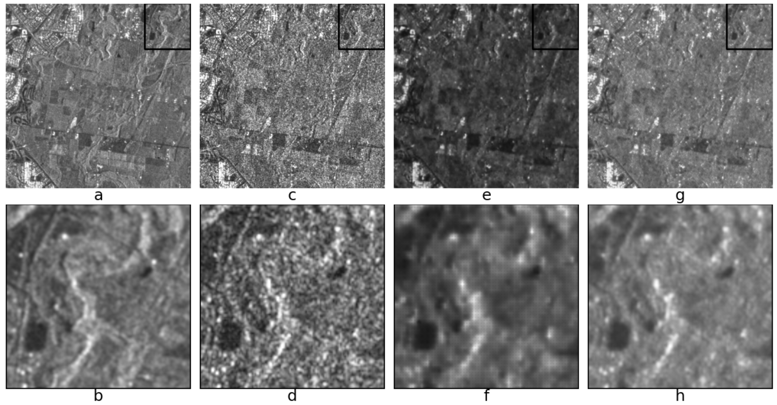
Models 94 and 160 have been chosen among the pool of 240 trained models to exemplify the outcomes achieved in SAR image denoising. These specific models serve as representations showcasing the variance in performance within the autoencoder models. Comparing these two models presents the differences in their abilities to reduce speckle and preserve quality in SAR imagery. The performance comparison between Models 94 and 160 demonstrates stark differences in their efficacy. Model 94 exhibits lower mean values across metrics MSE, SSIM, PSNR, and ENL compared to Model 160, indicating poorer speckle reduction and less image fidelity. The standard deviation values, detailed in

Table 3. Comparison of Models 94 and 160.

Model	94	160
MSE mean $\left[\overline{{\phi }_1}\right]$	2936.850	262.986
SSIM mean $\left[\overline{{\phi }_2}\right]$	0.460	0.696
PSNR mean $\left[\overline{{\phi }_3}\right]$	13.758	24.252
ENL mean $\left[\overline{{\phi }_4}\right]$	12.830	18.085
MSE std $\left[D_{\overline{{\phi }_1}}\right]$	837.174	106.816
SSIM std $\left[D_{\overline{{\phi }_2}}\right]$	0.046	0.056
PSNR std $\left[D_{\overline{{\phi }_3}}\right]$	2.043	1.652
ENL std $\left[D_{\overline{{\phi }_4}}\right]$	2.404	2.851

, consistently reflect higher variability in Model 94 results across all metrics.

Model 94 is structured with six convolutional layers and 64 filters per layer, using the ELU activation function and a batch size of 2. The model was trained with the binary crossentropy loss function and a learning rate of 0.005. In contrast, Model 160 features a four-layer convolutional architecture with 32 filters per layer, also employing the ELU activation function, but with a batch size of 4. Like Model 94, it was trained with binary crossentropy as the loss function and a learning rate of 0.005. These two models, with their different layer configurations and filter sizes, show significant differences in their performance metrics, particularly in terms of speckle reduction and image fidelity.

Figure 5 illustrates the filtered SAR images obtained from Models 94 and 160, showcasing their impact on speckle reduction. In the first column, the ground truth SAR image is displayed, accompanied by a zoomed-in view of the selected region. In the second column, the SAR image with speckle is presented, accompanied by a zoomed-in view. In the third column, the SAR image filtered using Model 94 is presented, accompanied by a zoomed-in view. Finally, the fourth column exhibits the SAR image filtered with Model 160, followed by the zoomed-in view. This comparative visualization of the denoising effects of the two models on SAR imagery highlights their varying abilities to mitigate speckle.

4.2. Pareto Frontier

A set of autoencoder architectures, capable of simultaneously optimizing performance across the four metrics, was identified through experimentation. To accomplish this multi-objective optimization task, we utilized the Multimodal Pareto Front Optimization methodology. This approach facilitated the exploration of the Pareto frontier, enabling the identification of solutions that achieved the best possible trade-offs among the competing objectives. The Multimodal Pareto Front Optimization methodology allowed for a comprehensive analysis of the trade-offs between MSE, SSIM, PSNR and ENL, leading to the discovery of a group of architectures that demonstrated superior performance across all metrics. This method enabled the identification of the optimal architectures and provided insights into the relationships between the different performance measures, shedding light on the balance required to achieve denoising in SAR images.

The Multimodal Pareto Front Optimization method is well suited when multiple, potentially conflicting objectives need to be simultaneously optimized. It aims to identify a set of solutions along the Pareto front that represents the trade-offs between these objectives. In our case, the Pareto front captures the trade-offs between minimizing MSE, maximizing SSIM, maximizing PSNR, and maximizing ENL values for the autoencoder architectures. Through the application of this method, we successfully obtained a subset of architectures that reside on the Pareto front and can be considered as prime candidates for further analysis. These architectures have demonstrated their potential to achieve a balanced trade-off between reconstruction quality (MSE, SSIM) and fidelity (PSNR, ENL) in the context of SAR image despeckling.

The scatter plot in Figure 6 showcases the dispersion of metrics across different autoencoder architectures trained for SAR image despeckling. In this visualization, red points present the models positioned closest to the Pareto frontier, indicating their superior performance between minimizing MSE while maximizing SSIM, PSNR and ENL values. These models showcase their potential as candidates exhibiting enhanced performance in SAR image despeckling.

Table 4. Autoencoder architectures belonging to the Pareto front.

Model	Conv Layers	Filters	Activation	Batch Size	Loss	Learning Rate
0	6	32	relu	2	mse	0.001
13	6	32	relu	8	mse	0.005
30	6	32	elu	2	mse	0.001
36	6	32	elu	4	mse	0.001
60	6	64	relu	2	mse	0.001
66	6	64	relu	4	mse	0.001
69	6	64	relu	4	bce	0.001
72	6	64	relu	8	mse	0.001
112	6	64	elu	16	bce	0.005
123	4	32	relu	2	bce	0.001
153	4	32	elu	2	bce	0.001
160	4	32	elu	4	bce	0.005
166	4	32	elu	8	bce	0.005
180	4	64	relu	2	mse	0.001
183	4	64	relu	2	bce	0.001
213	4	64	elu	2	bce	0.001
232	4	64	elu	16	bce	0.005

includes a subset of the optimal autoencoder architectures comprising the Pareto frontier. This subset includes 17 distinct models, each characterized by specific configurations of convolutional layers, filter sizes, activation functions, batch sizes, loss functions, and learning rates. The architectures showcased in the table exemplify the combinations of hyperparameters that have demonstrated superior performance across evaluation metrics. These architectures represent promising candidates for exploration in SAR image despeckling applications.

Table 5. Metric results for optimum models.

Model	MSE Mean $\left[\overline{{\mathit{\phi }}_1}\right]$	SSIM Mean $\left[\overline{{\mathit{\phi }}_2}\right]$	PSNR Mean $\left[\overline{{\mathit{\phi }}_3}\right]$	ENL Mean $\left[\overline{{\mathit{\phi }}_4}\right]$
0	290.423	0.687	23.883	19.500
13	290.399	0.653	23.810	20.758
30	258.975	0.680	24.353	19.524
36	258.077	0.676	24.391	19.193
60	258.506	0.670	24.401	20.507
66	262.700	0.670	24.299	20.574
69	290.987	0.662	23.838	20.902
72	260.597	0.679	24.372	20.298
112	260.007	0.680	24.399	19.061
123	260.631	0.693	24.325	18.653
153	264.949	0.696	24.195	18.119
160	262.986	0.696	24.252	18.085
166	264.689	0.695	24.216	18.272
180	256.701	0.690	24.352	19.376
183	261.251	0.692	24.340	19.446
213	269.763	0.693	24.156	18.319
232	280.138	0.694	24.002	18.437

presents a overview of the performance metrics associated with 17 autoencoder models situated on the Pareto front. These metrics serve as indicators of the image quality enhancement capabilities of the evaluated models. The table allows for a comparison of the relative performance of the models based on their respective metrics, providing insights into their potential for reducing image noise.

The set of 17 optimal models revealed insights into their performance based on used metrics. The MSE values ranged from 290.42 to 256.70, indicating different levels of reconstruction accuracy achieved by the models. The SSIM varied from 0.653 to 0.696, highlighting the diversity in the preservation of structural information between the reconstructed and original images. The PSNR values spanned from 23.88 to 24.40, reflecting the models abilities to minimize noise and retain image fidelity. Finally, the ENL values ranged from 19.50 to 18.07, demonstrating variations in the effectiveness of speckle reduction among the optimal models.

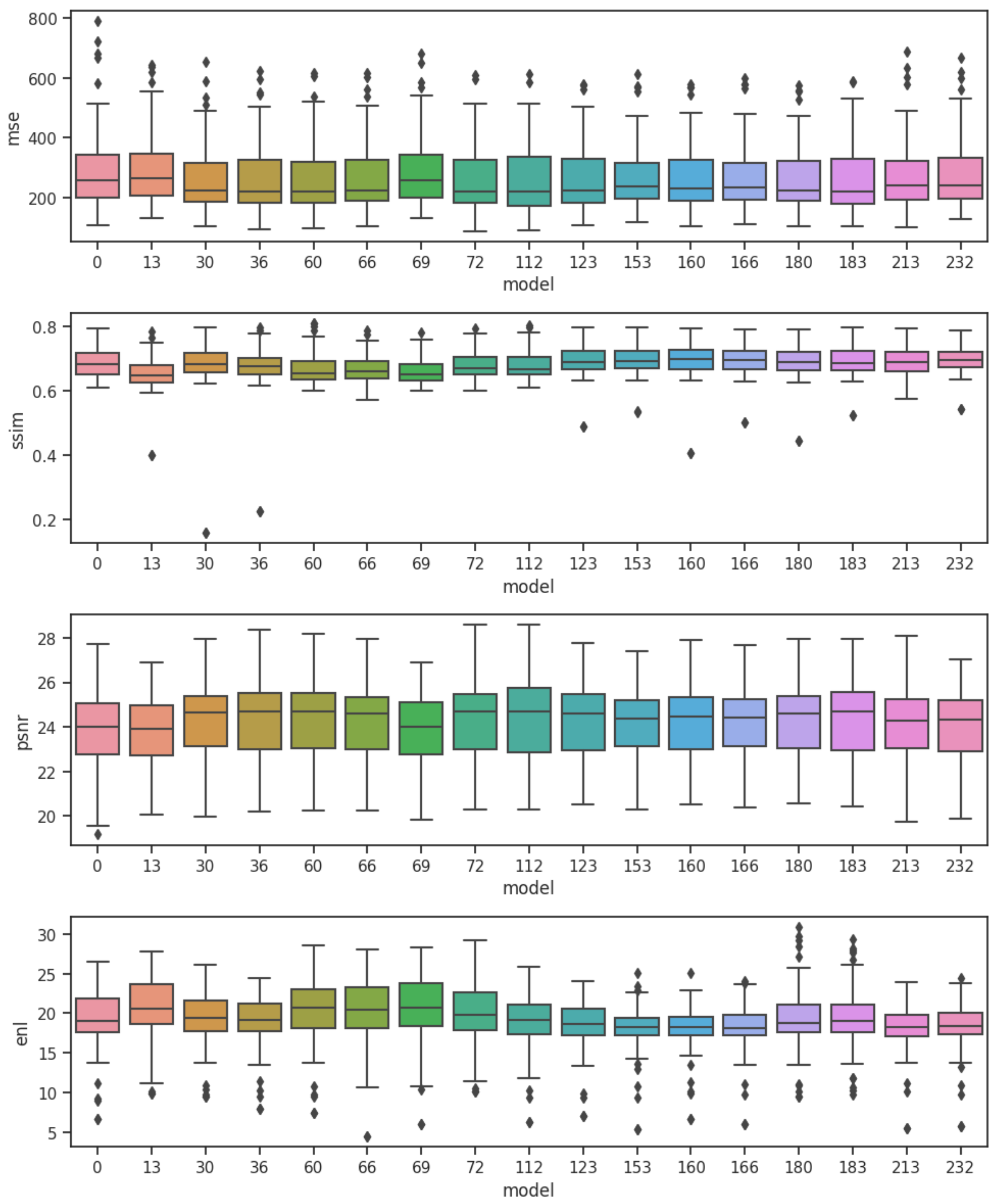
The box plot visual representation of the 17 autoencoder models on the Pareto front presents the variability in the performance metrics of these models (Figure 7). The plot reveals a consistency in the metrics across the 17 models, suggesting a level of uniformity in their image enhancement capabilities. The closely clustered box plots indicate that the models demonstrate similar levels of performance in terms of MSE, SSIM, PSNR and ENL in reducing speckle and improving the overall quality of the processed images.

After reevaluating the p-values for the 17 models identified as optimal following the ANOVA analysis, the obtained results are as follows. The p-value for MSE is 0.334, indicating no significant difference among the models in terms of MSE. However, for SSIM and ENL, the p-values are extremely small, approximately 2.4 × 10⁻¹⁴ and 2.9 × 10⁻¹⁶, respectively. These values present evidence against the null hypothesis, suggesting substantial differences between the models concerning SSIM and ENL. Concerning PSNR, the obtained p-value is 0.137, indicating no significant difference among the models. These findings highlight the importance of SSIM and ENL, showcasing clear disparities among the models, implying that some models perform significantly better in preserving structural similarity and homogeneity in filtered SAR images compared to others.

4.3. Confidence Intervals

The use of confidence intervals aids in the assessment of the variability and precision of the estimated population parameters, enabling us to make inferences about the effectiveness of different models in denoising SAR imagery. By incorporating confidence intervals in the ANOVA analysis, it can identify the range of plausible values for the means of the evaluated metrics, facilitating a comparison of the performance of various autoencoder architectures. Additionally, the insights garnered from the confidence intervals enable the identification of statistically significant differences in the performance of different models, providing a reliable basis for selecting the most effective autoencoder configuration.

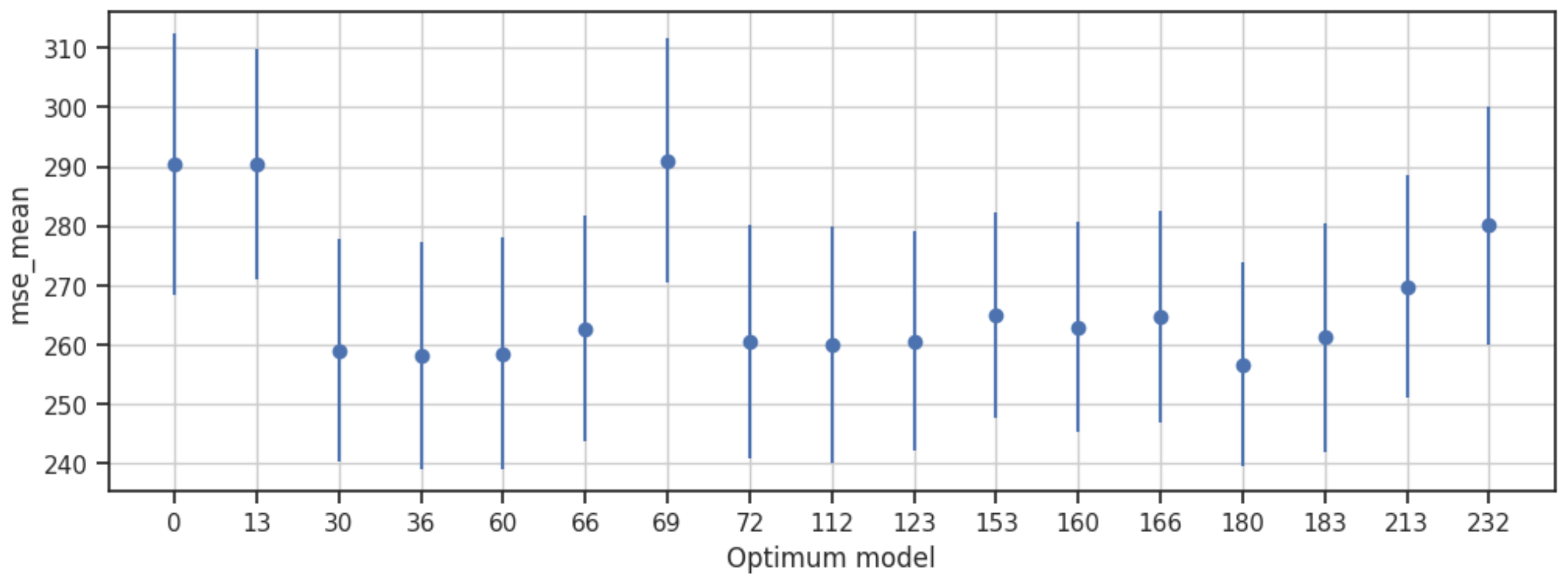
Mean Squared Error (MSE)—The confidence intervals indicate that the true population mean of the reconstruction error is expected to lie between 238.94 and 312.37, with a margin of error of 19.10. This suggests notable variability in the performance of the autoencoder models, emphasizing the need for further optimization to minimize the error range and improve the accuracy of the reconstructed images (Figure 8).

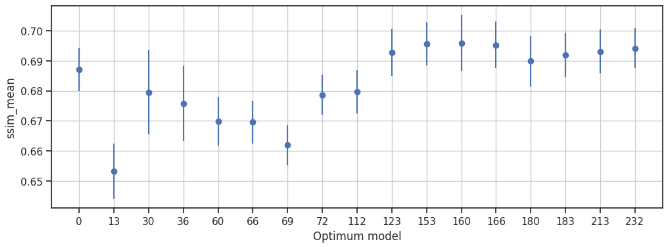
Structural Similarity Index (SSIM)—The confidence intervals for the SSIM range from 0.64 to 0.71, with a small error of 0.008, indicating a relatively precise estimate of the population SSIM index. These results suggest that the selected autoencoder models are effective in preserving the structural information of the images, ensuring minimal loss of details during the denoising process (Figure 9).

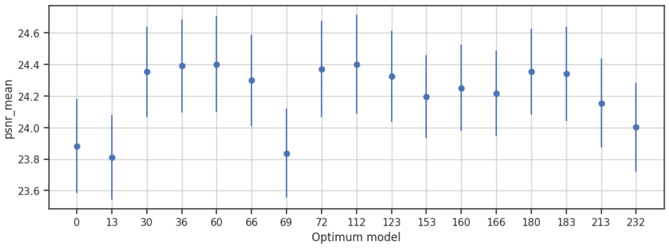
Peak Signal-to-Noise Ratio (PSNR)—The narrow confidence interval range of 23.54 to 24.71, with an error of 0.29, highlights the accuracy of the reconstructed images compared to the original data. These results underscore the efficiency of the models in maintaining the image quality and minimizing the signal distortion caused by speckle (Figure 10).

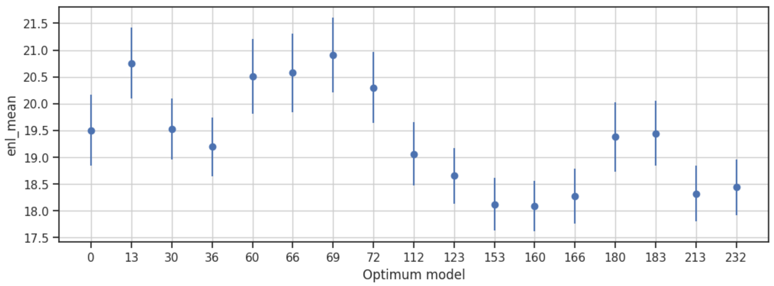
Equivalent Number of Looks (ENL)—The confidence intervals for ENL range from 17.61 to 21.60, with an error of 0.60, indicating moderate variability in the estimated ENL values. These results suggest that the selected autoencoder models effectively reduce speckle within this range, demonstrating their capability in improving the quality of SAR images (Figure 11).

The analysis of the confidence intervals for the metrics underscores the trade-offs and interdependencies between various performance indicators. While the models showcase a considerable range of performance variations, it is evident that the selected autoencoder architectures have demonstrated a capacity to effectively reduce speckle while preserving essential image details. The wide confidence intervals for MSE and ENL present the need for further fine-tuning and optimization to minimize the reconstruction error and enhance the noise reduction capabilities. The narrow confidence intervals for SSIM and PSNR reflect the models’ success in maintaining structural information and minimizing signal distortion, illustrating their robustness in preserving the overall image quality. These insights not only reinforce the efficacy of the chosen models in mitigating speckle but also provide directions for refining the autoencoder architectures to achieve superior performance.

4.4. The Best Model

The process of selecting the most optimal SAR image denoising autoencoder model from the pool of 17 preselected models involved a systematic ranking system based on evaluation metrics. Each metric, MSE, SSIM, PSNR and ENL, was utilized to establish a scoring position for every model. For MSE, the models were arranged in ascending order based on their performance, with the lowest MSE value (

Table 6. Performance positions for MSE.

Model	MSE Mean $\left[\overline{{\mathit{\phi }}_1}\right]$	MSE Mean Ranking $\left[\mathcal{R}\overline{{\mathit{\phi }}_1}\right]$
180	256.701	1
36	258.077	2
60	258.506	3
30	258.975	4
112	260.007	5
72	260.597	6
123	260.631	7
183	261.251	8
66	262.700	9
160	262.986	10
166	264.689	11
153	264.949	12
213	269.763	13
232	280.138	14
13	290.399	15
0	290.423	16
69	290.987	17

) assigned to position 1 and consecutively numbered up to 17, representing the least efficient model in this metric. Conversely, for SSIM, PSNR, and ENL, which exhibit superior performance with higher values, the models were ranked in descending order, assigning position 1 to the model with the highest score in each metric. This methodology proposed in Section 3.6 and its Algorithm 1 allowed for the creation of a comprehensive table presenting the positions of all 17 models across the four evaluation metrics, enabling a clear delineation of each model’s relative performance for these evaluation criteria.

After establishing the individual performance positions of the 17 autoencoder models across each of the four metrics, an assessment of their collective performance was conducted by summing up the positions acquired by each model across these metrics. This summation approach aggregates the positional ranks obtained by each model for metrics such as MSE, SSIM, PSNR and ENL. For example, in

Table 7. Metric performance position and total cumulative position.

Model	MSE Mean Ranking $\mathcal{R}\overline{{\mathit{\phi }}_1}$	SSIM Mean Ranking $\mathcal{R}\overline{{\mathit{\phi }}_2}$	PSNR Mean Ranking $\mathcal{R}\overline{{\mathit{\phi }}_3}$	ENL Mean Ranking $\mathcal{R}\overline{{\mathit{\phi }}_4}$	Total Mean Score
60	3	14	1	4	22
180	1	8	6	9	24
30	4	11	5	6	26
72	6	12	4	5	27
36	2	13	3	10	28
112	5	10	2	11	28
183	8	7	7	8	30
123	7	6	8	12	33
66	9	15	9	3	36
160	10	1	10	17	38
166	11	3	11	15	40
153	12	2	12	16	42
213	13	5	13	14	45
232	14	4	14	13	45
0	16	9	15	7	47
69	17	16	16	1	50
13	15	17	17	2	51

, consider Model 60; it secured position 3 for MSE, position 14 for SSIM, position 1 for PSNR and position 4 for ENL, resulting in a cumulative position total of 22 across all metrics. This cumulative position total serves as an amalgamated performance measure across multiple evaluation criteria. Lower cumulative position totals imply a superior and well-rounded performance across all metrics. Thus, the model with the lowest cumulative position total emerges as the prime candidate exhibiting the most robust and balanced performance across the spectrum of evaluation metrics.

The procedure of scoring by position based on standard deviations is reiterated to further assess the consistency of performance of the 17 pre-selected autoencoder models across all evaluation metrics. This approach, akin to the prior methodology utilized with mean values, involves assigning positions based on the standard deviations of the evaluation metrics. For instance, Model 180 showcases a total positional value for the arithmetic mean of metrics at 24 and a total positional value for the standard deviation of metrics at 29, as depicted in

Table 8. Total positions of mean and standard deviation.

Model	Total Mean Score	Total Std Score	Total Score $\left[\mathit{S}\right(\mathit{M}\left)\right]$
180	24	29	53
153	42	12	54
166	40	20	60
160	38	24	62
123	33	30	63
30	26	40	66
72	27	44	71
36	28	44	72
183	30	42	72
213	45	27	72
112	28	45	73
232	45	30	75
60	22	54	76
66	36	40	76
13	51	39	90
69	50	41	91
0	47	51	98

. These cumulative positional values, indicating both mean and standard deviation assessments, are combined to establish a definitive overall total value. The objective is to identify the most optimal model, evident through the model achieving the lowest total sum of positional values.

The analysis identifies Model 180 as the most optimal autoencoder architecture, showcasing a total positional value of 53. This evaluation integrates both mean and standard deviation positional assessments across the four evaluation metrics. This model exhibits superior consistency, achieving a lower total sum of positional values across the spectrum of evaluation criteria. Model 180 stands out as the most promising candidate among the 17 pre-selected autoencoder models, displaying proficiency in optimizing performance in SAR image despeckling.

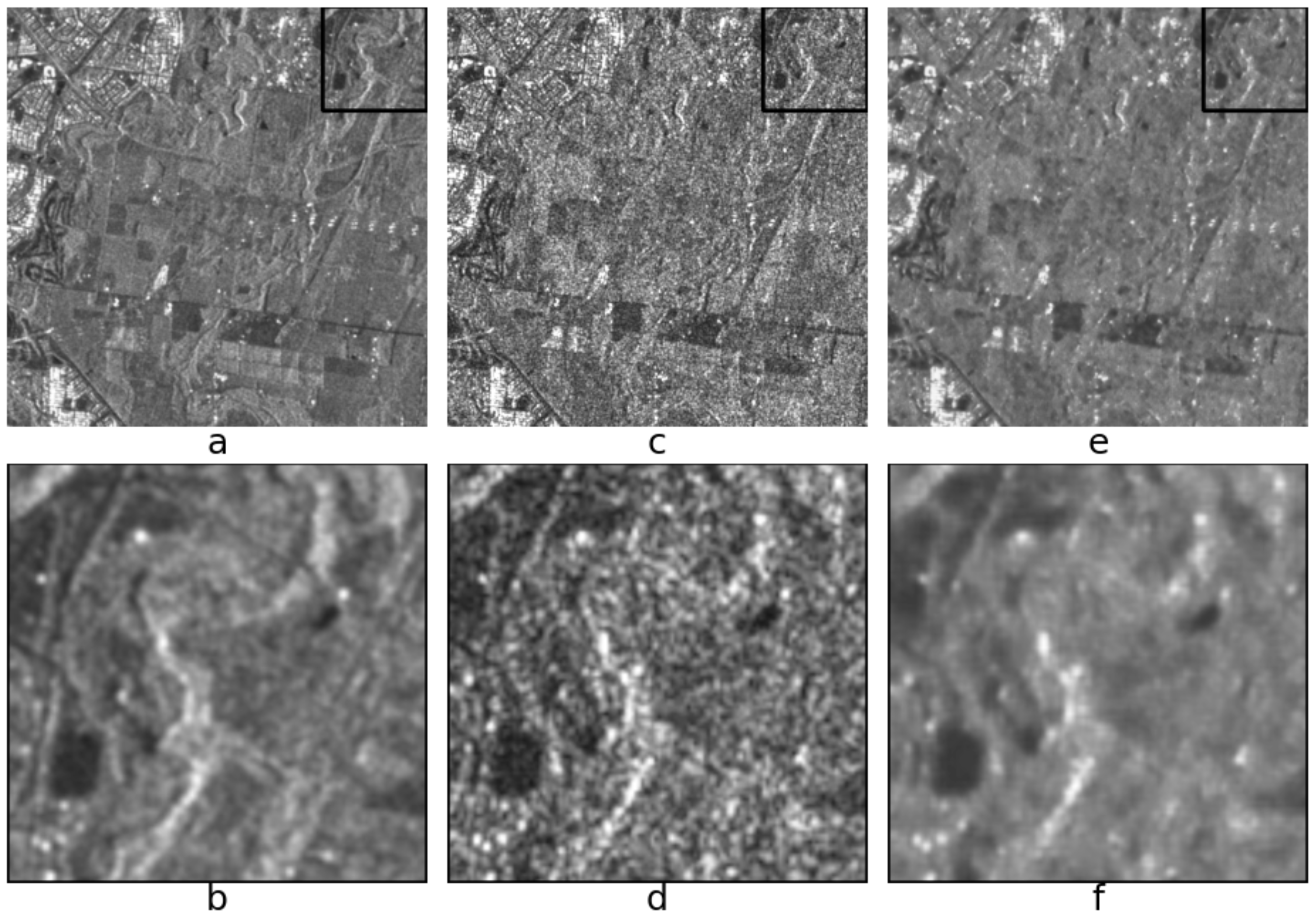
The results illustrated in Figure 12 display the outcomes achieved by Model 180 with the minimal $S\left(M\right)=53$. The images are organized in columns, presenting an image with its corresponding zoomed-in region selected within the box. The first column exhibits the ground truth images devoid of speckle. The second column presents images affected by speckle. Finally, the third column demonstrates the filtered images produced by the selected autoencoder model. This visualization enables a full comparison, highlighting Model 180’s ability to denoise speckle images.

Visual analysis of the images generated by Models 0, 36 and 180 provides information on their respective performances, particularly when ranked from the positions of the least favorable Model 0 to the intermediate Model 36 and the most favorable Model 180 according to the classification system. Examining Figure 13, it is evident that Model 180, positioned as the top-ranking model, exhibits a commendable reduction in mottling, positioning itself as a strong candidate for best model. In particular, images generated by Model 180 show a significant improvement in image quality, effectively suppressing unwanted speckle artifacts. However, it is essential to recognize that both Model 0, the lowest ranked model, and Model 36, the middle ranked model, also demonstrate considerable reductions in speckle levels in SAR images. While visual analysis positions Model 180 as a potential optimal choice, the competent noise removal performance of Models 0 and 36 highlights their effectiveness in mitigating speckle.

Notably, Model 180, positioned at the top across all metrics in Table 7, attains the lowest MSE (1), highest SSIM (8), considerable PSNR (6), and superior ENL (9). This consistently high ranking suggests that Model 180 excels in minimizing pixel-wise errors, preserving structural information, enhancing signal quality, and maintaining a high equivalent number of looks in the images, indicating its visual superiority. Conversely, Model 36, occupying the intermediate position, displays moderately higher positions across MSE (2), SSIM (13), PSNR (3), and ENL (10). While not surpassing Model 180, Model 36 still showcases commendable performance, positioning itself as a competitive choice with perceptually pleasing results. Finally, Model 0, situated at the lowest rank, exhibits the highest positions across MSE (16), SSIM (9), PSNR (15), and the lowest ENL (7). These results signify increased pixel-wise errors, lower structural similarity, reduced signal quality, and a diminished equivalent number of looks in comparison to the other models.

The consistent pattern of Model 180 outperforming both Model 36 and Model 0 across all metrics underscores its visual superiority. The intermediate performance of Model 36 suggests a satisfactory compromise, while the lowest-ranking Model 0 indicates suboptimal outcomes in terms of image analysis metrics. These quantitative findings align with the visual observations, reinforcing the efficacy of the ranking system and providing insights into the models’ performance for image denoising.

5. Discussion and Future Work

This section provides an analysis of the results obtained from the autoencoder models trained for SAR image despeckling. This section first discusses the key findings and insights derived from the evaluation of the models, followed by an exploration of potential improvements and directions for future research. The subsections that follow delve into the significance of the results, the advantages of the proposed methodology, and the opportunities for advancing this area of study through continued innovation and refinement.

5.1. Discussion of Results

The results of this study provide valuable insights into the effectiveness of autoencoders for speckle reduction in Synthetic Aperture Radar (SAR) images. The use of 240 distinct autoencoder models, each trained with different combinations of hyperparameters, allowed for a comprehensive evaluation of their performance across multiple image quality metrics, such as MSE, SSIM, PSNR, and ENL.

The significant variability observed in the performance of the different models underscores the complexity of SAR image despeckling. While all models demonstrated some level of speckle reduction, the models selected based on the Pareto frontier achieved the best trade-offs between noise reduction and image fidelity. Specifically, the results revealed that models with lower MSE values also tended to have higher SSIM, PSNR, and ENL values, indicating better preservation of image features and overall image quality. This highlights the delicate balance between reducing speckle and maintaining the essential spatial information in SAR images, which is critical for downstream analysis.

The role of hyperparameter selection was crucial in determining the performance of the models. As shown by the ANOVA analysis, certain configurations of hyperparameters—such as the number of convolutional layers, the choice of activation function, and the learning rate—had a significant impact on the models’ ability to reduce speckle and preserve structural information. The wide range of performance outcomes, from models with MSE values as low as 256.70 to those as high as 18,776.14, suggests that careful tuning of these hyperparameters is essential for optimizing autoencoder performance in SAR image processing.

One of the key findings of this study was the identification of the Pareto frontier, which served as a useful method for selecting models that exhibited the best performance across multiple objectives. The models residing on the Pareto frontier demonstrated superior overall performance, providing a set of promising candidates for further analysis and application. This approach not only helped in identifying the most optimal models but also revealed the inherent trade-offs between competing performance metrics, such as minimizing MSE while maximizing SSIM and PSNR. These trade-offs are crucial for practical applications, where different performance criteria may be prioritized depending on the specific goals of the task at hand.

The evaluation using a diverse set of 240 models allowed for a deep exploration of model performance and the identification of configurations that can generalize well across various SAR images. However, as the study was based on a single SAR dataset, further research should focus on testing the models on a wider variety of datasets to ensure their robustness in different operational contexts. This would also allow for the refinement of the models, improving their ability to generalize across different terrains, weather conditions, and acquisition scenarios.

The presence of outliers in the box plot graph represents models that exhibit performance significantly outside the expected range. In this case, the values outside of the range correspond to suboptimal models that fail to achieve optimal speckle reduction or image fidelity. These outliers may result from particular hyperparameter configurations that are not well suited for the task or models that struggle with specific data characteristics. The ratio of outliers is relatively low, indicating that the majority of models perform within the expected range. The impact of these suboptimal models on the overall denoising results is minimal, but their presence highlights the need for careful optimization of the hyperparameters to avoid configurations that lead to poor performance. These outliers reinforce the importance of fine-tuning the models to ensure consistent and high-quality denoising across all configurations.

5.2. Comparison with State-of-the-Art Algorithms

In the field of SAR image despeckling, several advanced algorithms have been developed to address the challenges posed by speckle noise while preserving the important features of the images. Among these, deep learning-based methods have gained significant attention due to their ability to learn complex patterns and handle noisy data effectively [8]. Specifically, CNN architectures [38] such as U-Net [12,39,40,41] and DeSpeckNet [13] have shown promise in reducing speckle noise while retaining high levels of image fidelity.

Compared to these state-of-the-art algorithms, the methodology proposed in this study presents a distinctive advantage by introducing analysis of variance (ANOVA) as a systematic and statistical approach for hyperparameter optimization in autoencoders. Unlike traditional methods that rely on trial-and-error techniques or heuristic approaches, ANOVA allows for a more precise selection of optimal hyperparameters, leading to improved model performance and efficiency in speckle reduction. This novel combination of ANOVA with deep learning models distinguishes this approach from other existing methods in the literature.

Additionally, while U-Net and DeSpeckNet utilize convolutional layers and skip connections for feature preservation during noise removal, the proposed methodology leverages Pareto frontier optimization, allowing for a balanced selection of models based on multiple performance metrics such as MSE, SSIM, PSNR, and ENL. This multi-objective evaluation provides a more comprehensive assessment of model performance compared to single-metric evaluations typically employed in state-of-the-art methods.

Furthermore, previous deep learning methods for SAR despeckling have often been limited by the size and quality of available datasets. In contrast, the approach presented in this study utilizes a large-scale dataset of 240 distinct models, each trained with varying hyperparameter configurations, ensuring a more robust and generalized solution to speckle reduction. This extensive training and evaluation across a diverse set of models contribute to the overall effectiveness of the proposed methodology in real-world applications.

By comparing the performance of this method with these leading algorithms, the study demonstrates that it not only achieves competitive results in terms of speckle reduction but also offers unique benefits in terms of model optimization, multi-objective evaluation, and robustness. These advantages position the proposed methodology as a promising alternative for advanced SAR image processing tasks.

5.3. Novelty of the Research

This study introduces an innovative approach by applying analysis of variance for hyperparameter optimization in autoencoders used for speckle reduction in SAR images. Unlike traditional methods that rely on heuristic or trial-and-error techniques, ANOVA systematically selects the optimal hyperparameters, significantly improving the precision and efficiency of the model optimization process. This application of ANOVA within the context of deep learning for SAR image processing is a novel contribution that enhances the rigor of model selection.

Additionally, the combination of advanced image quality metrics such as MSE, SSIM, PSNR, and ENL, alongside the identification of the Pareto frontier for model evaluation, provides a comprehensive and quantitative framework for assessing model performance. This approach not only highlights the autoencoders’ capability to reduce speckle but also their ability to preserve essential image features, which is crucial for SAR image analysis.

Furthermore, this research distinguishes itself by the extensive training of 240 different models, each with a distinct combination of hyperparameters. This large-scale evaluation provides a robust foundation for identifying the best-performing autoencoders, offering a level of depth not commonly seen in the existing literature on SAR image despeckling. The exhaustive nature of this study and the diversity of configurations explored are key factors that contribute to its originality.

The methodology presented here is not only focused on noise reduction but also on the systematic optimization of models through a defined, measurable process. The novel combination of ANOVA for hyperparameter tuning, Pareto frontier optimization, and extensive model training and evaluation provides a unique and rigorous methodology for SAR image despeckling, offering valuable insights into model performance and optimization that have not been previously explored in such detail within this domain.

5.4. Future Work

Building on the results presented in this study, several directions for future work can be pursued to further enhance SAR image despeckling and expand the application of deep learning techniques in this field.

While the current study focused on autoencoders, future research could explore other deep learning architectures, such as Generative Adversarial Networks (GANs), which have shown promise in image denoising tasks. Investigating the integration of GANs with autoencoders for SAR image despeckling could lead to improved noise reduction while maintaining image fidelity. Additionally, attention mechanisms and transformer-based models could be examined to capture more complex spatial relationships in SAR images.

The study used single-polarization data for training and evaluation. Future work could extend this approach to incorporate multi-temporal and multi-polarization SAR data, which are widely available and contain rich information for more accurate speckle reduction and change detection. This would enhance the generalization capability of the models and provide a more robust solution for real-world SAR image processing, particularly in dynamic environments.

Although ANOVA provided valuable insights for hyperparameter optimization, alternative optimization techniques such as Bayesian Optimization or Genetic Algorithms could be explored to further fine-tune model parameters. These methods may offer more efficient solutions by intelligently exploring the hyperparameter space, potentially leading to even better performance in speckle reduction.

6. Conclusions

The ANOVA analysis of various autoencoder models for SAR image despeckling emphasized the role of different filtering architectures in influencing the denoising capabilities and overall model performance. The results highlighted performance variations among the models, underlining the importance of architecture and hyperparameter configurations. The selection process focuses on identifying models on the Pareto frontier based on the best performance across multiple metrics. These findings emphasize the potential of advanced autoencoder models in significantly enhancing the efficiency and effectiveness of SAR image despeckling.

A subset of autoencoder architectures from the Pareto front demonstrated the ability to balance trade-offs between image quality metrics, achieving denoising while preserving fidelity. The wide range of MSE, SSIM, PSNR, and ENL values among the 17 optimal models provides valuable insights into performance characteristics and informs future image processing advancements.

Integrating confidence intervals into the ANOVA analysis was key to assessing the variability and precision of the models. Wide confidence intervals for MSE and ENL highlight the need for further optimization, while narrow confidence intervals for SSIM and PSNR confirm the models’ effectiveness in preserving structural information and minimizing signal distortion. These findings underscore the importance of leveraging confidence intervals for informed decisions and refining autoencoder architectures for improved SAR image denoising.