Bi-Objective Integrated Scheduling of Job Shop Problems and Material Handling Robots with Setup Time

Abstract

This work investigates the bi-objective integrated scheduling of job shop problems and material handling robots with setup time. The objective is to minimize the maximum completion time and the mean of earliness and tardiness simultaneously. First, a mathematical model is established to describe the problems. Then, different meta-heuristics and their variants are developed to solve the problems, including genetic algorithms, particle swarm optimization, and artificial bee colonies. To improve the performance of algorithms, seven local search operators are proposed. Moreover, two reinforcement learning algorithms, Q-learning and SARSA, are designed to help the algorithm select appropriate local search operators during iterations, further improving the convergence of algorithms. Finally, based on 82 benchmark cases with different scales, the effectiveness of the suggested algorithms is evaluated by comprehensive numerical experiments. The experimental results and discussions show that the genetic algorithm with SARSA is more competitive than its peers.

1. Introduction

Within production organizations, scheduling plays an extremely important role, especially in the context of manufacturing planning [1]. The efficacy of a manufacturing planning system is determined by the performance of its scheduling approach. Scheduling is categorized based on the job environment, job characteristics, and optimization criteria [2]. The job environment can also be referred to as a machine environment. Scheduling is further divided into single-stage and multi-stage based on machine setup. In single-stage scheduling, there is only one machine and a few tasks, whereas in multi-stage scheduling, there are multiple machines and jobs.

Job Shop Scheduling (JSP) is a critical issue in resource allocation. Resources in this context are referred to as machines, and the basic units of work are called jobs. Each job can consist of several sub-tasks, known as operations, which are interconnected by priority constraints. JSP is a significant class of nondeterministic polynomial-time (NP) problems, similar to the traveling salesman problem [3].

In a static JSP, deterministic jobs are handled by a pre-determined number of machines. The sequence of actions for every individual job is pre-established, and each task must be completed exactly once. It is not possible to perform two tasks simultaneously on the same machine and must wait until the previous operation is completed on that machine. Arranging the operating slots on the device, or computer, is referred to as a schedule. The maximum completion time (makespan) is one of the most common objectives for the JSP.

The bi-objective integrated scheduling of job shop problems and material handling robots (MHR) with setup time, known as BI-JSP-MHR, is a generalization of production scheduling issues. Unlike the classic JSP, which does not consider transportation resources and assumes an unlimited number of MHRs. The BI-JSP-MHR takes into account the practical constraints of workshops. Workshops often have a finite number of MHRs due to the high costs and the limitations of the workshop layout. Setup time is an essential auxiliary factor required for different operations and processes to be carried out on a machine, and it plays a significant role in the overall cycle time of an operation. A shorter setup time can boost productivity by minimizing machine idle time between production runs. Conversely, excessive setup time can significantly slow down the production process, leading to higher costs and longer lead times for customers. Therefore, optimizing the concerned problems with setup time is a key factor in enhancing the efficiency and competitiveness of manufacturing operations. Consequently, research on BI-JSP-MHR aligns more closely with the actual conditions of production, making it highly significant in theoretical studies. BI-JSP-MHR must address two sub-issues: the selection of MHRs and the scheduling of tasks.

Due to the sequential logic constraints between the transport and processing stages, the problem is not easily decoupled. Compared with JSP, BI-JSP-MHR is significantly more challenging, as detailed below:

(1) In addition to the problem of scheduling for processing machines with operational constraints, it is also necessary to address the task assignment for the MHRs.

(2) There is a significant difference between the transport behavior of MHRs and that of machines. These actions are performed alternately, and there may be required waiting periods during execution. This leads to a more complex cascade effect in the calculation of the number of completed jobs.

(3) It is difficult to decouple the interdependence of processing tasks and transport tasks, which implies that a layered or decoupling mechanism might lose its optimal solution.

Clearly, BI-JSP-MHR is a more complex NP-hard problem than JSP. The complexity of BI-JSP-MHR makes it more challenging to study its intrinsic properties and solutions.

The novel contributions this work aims to make include the following:

(1) Establish a double-objective mathematics model for the integration of job shop problems and material processing robots.

(2) Improve different meta-heuristics, including Artificial Bee Colony (ABC), Genetic Algorithm (GA), and Particle Swarm Optimization (PSO), are developed to solve the problems.

(3) Seven local search operators based on problem features are devised for enhancing the quality of algorithms.

(4) Q-learning and SARSA-based local search operators are developed and embedded into meta-heuristics to select high-quality local search strategies.

The designed algorithms enable efficient solving of 82 benchmark instances with different sizes, which provides valuable insights for practical production applications.

The rest of this paper is organized as follows. Section 3 develops a double-objective mathematics model for the integration of the job shop problem and material processing robot. Section 4 presents three meta-heuristics with reinforcement learning-based improved strategies in detail. Section 5 presents experimental results and comparisons. Finally, this study is summarized, and future research directions are suggested in Section 6.

2. Literature Review

2.1. Fundamental Problems

To address the JSP, some classical optimization technologies like [4,5,6,7,8,9] and meta-heuristics are designed, e.g., Ant Colony Optimization (ACO) [10], GA [11], and PSO [12]. These meta-heuristics can get obtain solutions quickly. In addition, several Lourenço researchers built a Local Retrieval process using [12] for the JSP. Wang et al. [13], Pinson [14], and Cheng. [15] introduce several heuristic approaches. Moreover, a combined approach to optimize JSP was designed [16].

The JSP with AGV (JSP-AGV) is the extension of the JSP-MHR. The AGVs are specialized form of automated guidance machines. To minimize the makespan of JSP-AGV, Bilge and Ulusoy [17] establish a non-linear mixed-integer programming model and introduce a solution through the iteration technique. Deroussi et al. [18] put forth a neighborhood system. Erol et al. [19] devise a real-time multi-agent system that employs a negotiation/bidding mechanism among agents to create viable schedules. Kumar et al. [20] utilize two heuristics, one for machine selection and another for vehicle allocation. A mixed Integer Linear Programming (MILP) model and a Tabu Search (TS) algorithm, the innovation of the algorithm is the design of two-dimensional solution coding and a two-neighborhood mechanism [21]. Fontes et al. [22] develop a novel MILP model to address modest-sized instances. Fontes et al. [23] propose an integrated method combining PSO with simulated annealing. Nageswara et al. [24] introduce various initial methods to address the JSP-AGV. Lacomme et al. [25] model the JSP-AGV using a distinct preclusive graph and apply a hybrid evolutionary algorithm. Ham [26] aims to refine the solutions for JSP-AGV. Yao et al. [27] craft an innovative sequential MILP model, demonstrating superior performance compared to other MILP models.

Chen et al. [28] introduce a hybrid PSO approach to address the integration challenge of machines and AGVs. Yao et al. [29] establish a novel mathematical model for the flexible job shop scheduling problem. With limited AGVS. Niu et al. [30] employ a novel multi-task chain scheduling algorithm based on capacity prediction to solve the AGV dispatching problem in an intelligent manufacturing system. Hu et al. [31] employ the “first-in, first-out” heuristic to allocate the optimal AGV for every shipping assignment and then seek out the best local solutions. Yuan et al. [32] and Wen et al. [33] take into account the constraints of machinery, tasks, and AGVs, addressing the adaptable multi-objective job shop scheduling challenge involving AGVs using an enhanced NSGA-II algorithm. Goli et al. [34] explore the role of AGVs in Cellular Manufacturing Systems and develop an imprecise linear–integer programming model to it. The aim of this research is to reduce the production cycle time and the movement within intercellular areas.

2.2. Research Methods

Classic swarm and evolutionary algorithms, such as ABC, GA, and PSO, have been extensively applied to solve variant combination optimization problems. Numerous studies, including those by Liu et al., Huang et al., Fu et al., Qiao, Liu, and Cao, have employed these algorithms [35,36,37,38,39,40,41]. Yu et al. [42] employ GA and ABC to address dynamic surgery scheduling problems with fuzzy processing and setup times. Furthermore, Yu et al. [43] introduce an ABC algorithm based on Deep Q-Network (DQN). For addressing multi-objective heterogeneous USV scheduling problems. Lin et al. [44] use GA and PSO. To solve the urban traffic light scheduling with eight phases. GA, PSO, and Differential Evolution (DE) are proposed to address the multi-objective urban traffic light scheduling problem [45].

Q-learning, a widely utilized method in Reinforcement Learning (RL), has garnered significant attention across several articles [46,47,48]. Ensemble Q-learning has demonstrated the ability to enhance the performance of meta-heuristics. Li et al. [49] develop an ABC algorithm integrated with Q-learning and local search to tackle permutation flow shop scheduling problems. Chen et al. [50] incorporate Q-learning into GA, to realize intelligent parameter adjustment. Shen et al. [51] propose a novel memetic algorithm based on Q-learning for scheduling multi-objective dynamic software projects. Hsieh et al. [52] present an optimal swarm and optimal approach for the scheduling of economic problems. Gao et al. [53] introduce a novel approach that embeds Q-learning into meta-heuristics for the scheduling of unmanned ships.

Despite these investigations, further research is warranted for the problem at hand. As many scholars have noted, BI-JSP-MHR represents an advanced form of the conventional JSP. However, incorporating MHRs into the scenario can significantly alter the scheduling dynamics, and in some instances, the scheduling of MHRs might take precedence.

3. Problem Description

3.1. Problem Description

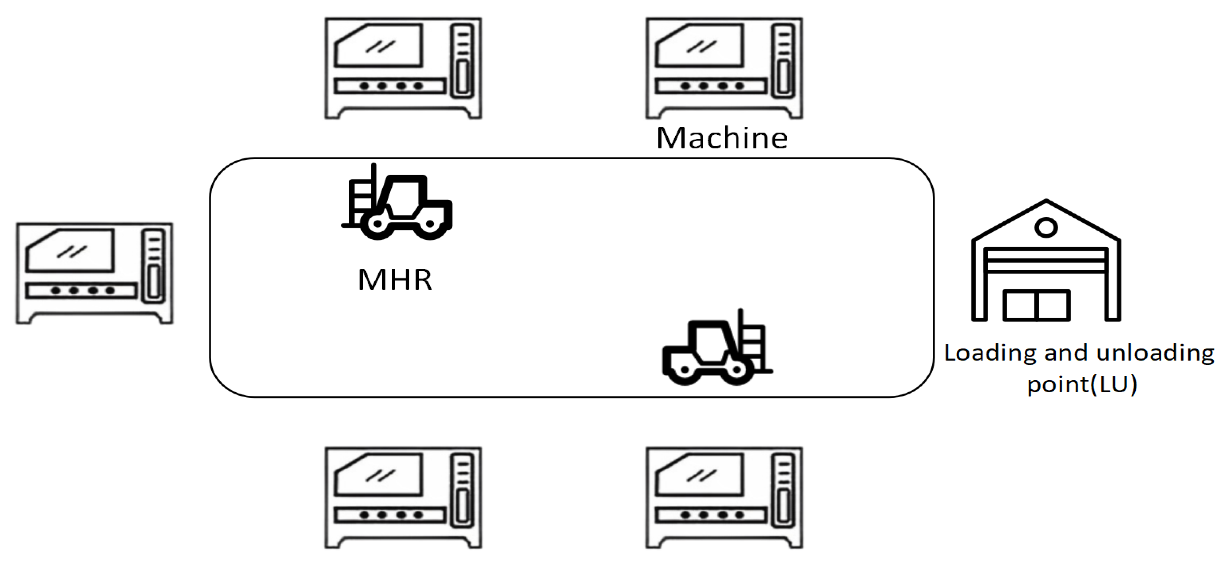
This study establishes a two-objective mathematical model to describe the integration of the job shop problem and the material handling robot with setup time. In the problem, part of the work is processed on certain machines, with each job comprising more than one operation. The MHR is responsible for transporting jobs. The work initiates at the Loading and Unloading (LU) station, which is located at a certain distance from the machinery. The MHR transportation takes time, and the movement of the MHR can be categorized into empty and loaded trips. An empty trip refers to the MHR’s journey from its current position to the designated machine to pick up a job, while a loaded trip is the MHR’s movement from picking up a job to delivering it to the destination machine. Figure 1 illustrates a production scenario with two MHRs and five machines. Our goal is to assign the most suitable processing machine and MHR to each job. Then, determine the order in which operations are performed on both the machines and the MHRs to minimize the objective. Specifically, once the final step in the work process is completed, an MHR is scheduled to deliver the finished product to the warehouse where finished goods are stored. Although transportation time is not included in the processing time of the job, it is crucial to monitor the MHR’s loading and unloading states.

The BI-JSP-MHR meets the following conditions:

(1) At time 0, all machines and MHRs are available.

(2) The time of loading and unloading is included in the transportation time.

(3) Each machine can handle a maximum of one operation.

(4) Each MHR can carry a maximum of one job.

(5) It is not possible to pre-empt an MHR when a transport task has begun.

(6) All MHRs have a fixed velocity, and the transmission time depends only on the location of the job.

(7) Each job can only be handled on one machine and can only be carried by one MHR when it is transferred from one machine to another. Once a job begins, it cannot be stopped until finished.

(8) After completion, work is returned to LU, but time is not taken into account.

(9) Different tasks have different setup times on the same machine.

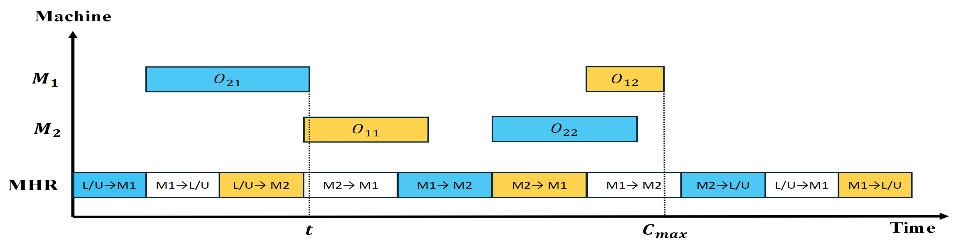
Figure 2 offers a visual representation of a Gantt chart for BI-JSP-MHR involving two jobs, two machines, and one MHR. Initially, the MHR moves $J_2$ to $M_1$, and then $M_1$ starts processing $O_{21}$. Following it, the MHR has to travel to the loading/unloading area and transport $J_1$ to $M_2$. At time t, $J_2$ waits for the MHR transportation from $M_2$ to $M_1$, and then it can start transporting $J_2$ from $M_1$ to $M_2$. The following steps are executed in a similar way. Finally, the makespan, denoted as $C_{max}$, is defined as the completion time of $O_{12}$.

Setup time primarily refers to the time spent on preparatory activities, such as cleaning the machine and replacing fixtures, molds, and other auxiliary tasks, when the machine is processing the next operation [54]. Setup time can be classified into two types: sequence-independent setup time and sequence-dependent setup time. Sequence-independent setup time suggests that the setup time for a machine depends solely on the current operation and not on the previous operations of the same machine; thus, it can be considered independent and unaffected by other operations. However, typically, the setup time of an operation is related not only to the current operation but also to the previous operation of the machine. That is, the setup time is linked to the processing sequence of the operation. Different processing sequences of operations result in different setup times for the machine. In such cases, constraints on the sequence among operations should be considered when accounting for the number of machine setup times. The timing typically includes the time required to replace fixtures and molds, as well as the time needed for preparatory activities such as loading and unloading the job and starting the machine after the job arrives. Regardless of whether the auxiliary time is before or after the job’s arrival, it is treated as separate setup time. In this study, the setup time due to equipment setup after the job’s arrival during the waiting time is considered, which reduces the impact of waiting times on scheduling and aligns better with actual production conditions. Some example data on time are presented in

Table 1. Some example data about time.

Processing Time
Jobs		Operations			Machines
					$M_1$	$M_2$
Job 1		O1,1			6	—
		$O_{1,2}$			—	7
Transportation Time
Jobs		Operations			MHR
					L/U- $M_1$	$M_1$- $M_2$
Job 1		$O_{1,1}$			3	—
		$O_{1,2}$			—	2
Setup Time
Jobs		Operations			Machines
					$M_1$	$M_2$
Job 1		$O_{1,1}$			5	—
		$O_{1,2}$			—	4

.

Setup time is an essential auxiliary time required for different operations and processes to be carried out on a machine, and it plays a significant role in the overall cycle time of an operation. There are typically two approaches to handling setup time in the optimization scheduling problem of a workshop: one is to include it within the processing time; the other is to consider it separately, distinct from the processing time. As research evolves, treating setup time as a separate component is becoming a trend in the study of workshop scheduling problems. In this paper, we explore the impact of setup time on the classical job shop. By considering setup time as a separate component, the optimization of shop floor scheduling becomes more reflective of real-world workshop scenarios, enhancing its practical utility.

As shown in Figure 3, treating the setup time of the machine tools in the production process as part of the processing time effectively extends the production time. The number shown in Figure 3 is example time from Table 1. In this case, the shop scheduling problem only considers the processing time of the operation, which makes the final completion time of the operation closer to the actual production time, but the improvement in optimizing the shop scheduling problem is not particularly significant.

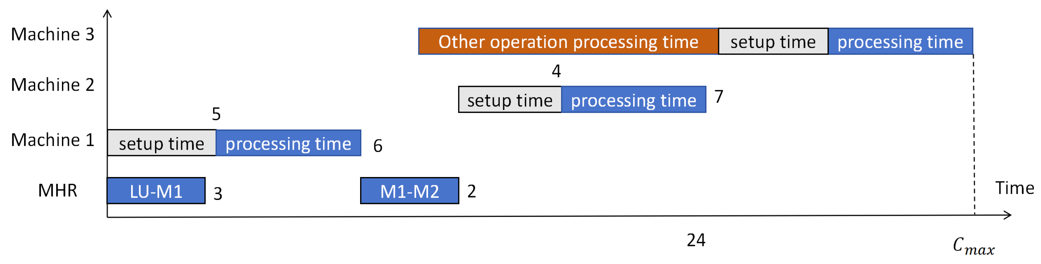
As shown in Figure 4, considering the setup time as a separate part makes it more aligned with real-world conditions of store production, making the optimization of store production scheduling more practically applicable.

3.2. Mathematical Model

The symbols employed in our model are detailed in

Table 2. The notations used in the model.

Notation	Description
n	Number of jobs
m	Number of machines
$o_i$	Number of operations of each job
v	Number of MHRs
i	Index of jobs
j	Index of operations
c	Index of machines
k	Index of MHRs
J	Set of n jobs, $\{J_1,J_2,\dots ,J_n\}$
M	Set of m machines, $\{M_1,M_2,\dots ,M_n\}$
O	Set of operations of job $J_i=\{O_{i,1},O_{i,2},\dots ,O_{i,n}\}$
V	Set of v MHRs, $\{V_1,V_2,\dots ,V_n\}$
D	A large positive number
$P{t}_{i,j}$	The processing time of operation $O_{i,j}$
$T{t}_{i,j}$	The travel time of transportation for operation $O_{i,j}$
$S{P}_{i,j}$	The start place of transportation for operation $O_{i,j}$
$E{P}_{i,j}$	The end place of transportation for operation $O_{i,j}$
$T_{c,c^{\prime }}$	The travel time from machine c to machine $c^{\prime }$
$C_i$	The completion time of job $J_i$
$C_{max}$	makespan
$ST{O}_{i,j}$	The start time of processing for operation $O_{i,j}$
$STL{O}_{i,j}$	The start time of loaded transportation for operation $O_{i,j}$
$x_{i,j,k}$	Binary variable that takes value 1 if MHR k is selected to perform the transportation for operation $O_{i,j}$, otherwise 0
$y_{i,j,i^{\prime },j^{\prime }}$	Binary variable that takes value 1 if operation $O_{i,j}$ is processed precedes operation $O_{i^{\prime },j^{\prime }}$ on the same machine, otherwise 0
$z_{i,j,i^{\prime },j^{\prime },k}$	Binary variable that takes value 1 if the transportation of operation $O_{i,j}$ is performed precedes operation $O_{i^{\prime },j^{\prime }}$ on MHR k, otherwise 0
$d_i$	The due date of $J_i$
$E/T$	Earliness and Tardiness
$S{E}_{i,j}$	The setup time operation $O_{i,j}$

.

The mathematical model can be described as follows:

$$minf(C_{max},E/T)$$

(1)

$$C_{max}=max(C_1,C_2,...,C_i,...,C_n)$$

(2)

$$C_i\ge {STO}_{i,o}+{Pt}_{i,o}+{SE}_{i,o},\forall i$$

(3)

$$E/T={\displaystyle \frac{{\sum }_{i=1}^n\left|c_i-d_i\right|}{n}}$$

(4)

$$\sum _{k\in v}{x}_{i,j,k}=1,\forall i,j,k$$

(5)

$${STO}_{i,j}\ge {STO}_{i^{\prime },j^{\prime }}+{Pt}_{i^{\prime },j^{\prime }}+{SE}_{i^{\prime },j^{\prime }}-D·y_{i,j,i^{\prime },j^{\prime }},\forall i,j,i^{\prime },j^{\prime },andj<j^{\prime }$$

(6)

$${STO}_{i,j^{\prime }}\ge {STO}_{i,j}+{Pt}_{i,j}+{SE}_{i,j}-D·(1-y_{i^{\prime },j^{\prime }i,j}),\forall i,j,i^{\prime },j^{\prime },andj<j^{\prime }$$

(7)

$${STO}_{i,j}\ge {STLO}_{i,j}+{Tt}_{i,j},\forall i,j$$

(8)

$${STLO}_{i,j}\ge {STO}_{i,(j-1)}+{Pt}_{i,(j-1)}+{SE}_{i,(j-1)},\forall i,jandj\ne 1$$

(9)

$$\begin{array}{c}{STLO}_{i,j}\ge {STLO}_{i^{\prime },j^{\prime }}+{Tt}_{i^{\prime },j^{\prime }}+T_{{{EP}_{i^{\prime },j^{\prime }}SP}_{i,j}}-D·(2-x_{i,j,k}-x_{i^{\prime },j^{\prime },k})-D·z_{i,j,i^{\prime },j^{\prime },k},\hfill \\ \hfill \forall i,j,i^{\prime },j^{\prime },andj<j^{\prime }\end{array}$$

(10)

$$\begin{array}{c}{STLO}_{i^{\prime },j^{\prime }}\ge {STLO}_{i,j}+{Tt}_{i,j}+T_{{{EP}_{i,j}SP}_{i^{\prime },j^{\prime }}}-D·(2-x_{i,j,k}-x_{i^{\prime },j^{\prime },k})-D·(1-z_{i,j,i^{\prime },j^{\prime },k}),\hfill \\ \hfill \forall i,j,i^{\prime },j^{\prime },andj<j^{\prime }\end{array}$$

(11)

$${STO}_{i,j}\ge 0,\forall i,j$$

(12)

$${STLO}_{i,j}\ge 0,\forall i,j$$

(13)

$$x_{i,j,k}\in \left\{0,1\right\},\forall i,j,k$$

(14)

$$y_{i,j,i^{\prime },j^{\prime }}\in \left\{0,1\right\},\forall i,j,k$$

(15)

$$z_{i,j,i^{\prime },j^{\prime },k}\in \left\{0,1\right\},\forall i,j,k$$

(16)

Constraint (1) presents the objective function, which aims to minimize both the makespan and the earliness and tardiness (E/T). Constraints (2) and (3) make sure that the makespan is longer than the finish time of any job. Constraint (4) calculates the ET. Constraint (5) provides for the allocation of traffic among the MHRs and for each transport to be allocated only one MHR. Constraints (6) and (7) indicate that each pair of concurrent operations is assigned a unique priority regardless of their processing time. Constraint (8) guarantees that a processing task must wait until the associated transport task has been finished before it can commence. Constraint (9) implies that the commencement of a transport activity is conditional on the completion of a previous activity, with the exception of the commencement of the work. Constraints (10) and (11) show the sequential relation of any two transports of the same MHR, ensuring that only one transport can be carried out by the MHR. The MHR will have an extra trip if the starting point of the ongoing transfer of the MHR and the last transmission are not the same. Constraints (12) and (13) ensure that the commencement times for both the processing and the loading of an operation are non-zero. Constraints (14), (15), and (16) define the decision variables.

3.3. Multi-Objective Optimization

The criterion of makespan has been extensively studied by researchers in the JSP domain. For manufacturing firms operating under a Just-In-Time (JIT) philosophy, adherence to due dates is paramount. The essence of JIT production lies in minimizing inventory, enhancing responsiveness, cash flow, and customer satisfaction. In the JIT paradigm, delivering early results in excess inventory, while late delivery leads to tardiness. Consequently, this study addresses the reduction of both the makespan in JSP and the average of earliness and tardiness. These objectives are mildly conflicting and have been referenced in existing literature.

4. Proposed Algorithm

4.1. Solution Representation

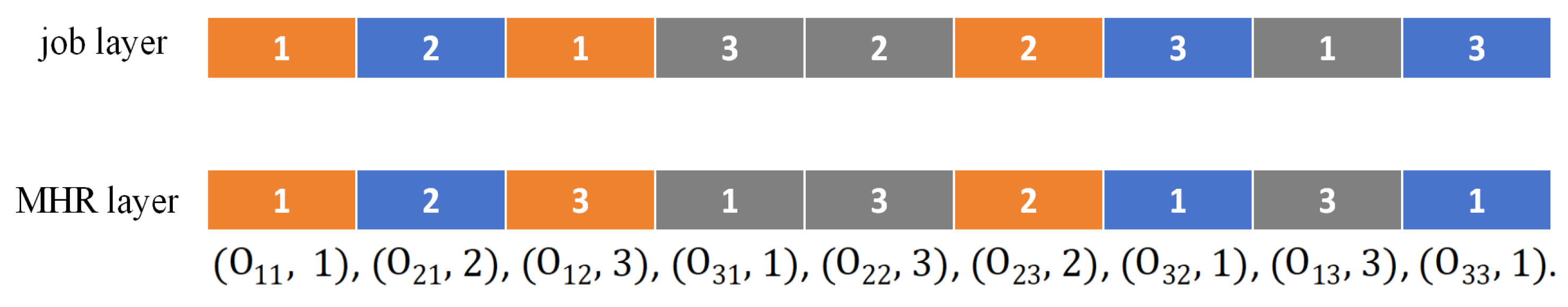
There are two sub-problems in BI-JSP-MHR, which are job scheduling and MHR scheduling. So, according to the characteristics of the concerned problem, a two-layer representation of the solution is used. The first layer (operation layer) is responsible for the expression of all operations. The second layer (MHR layer) is an indicator of the MHRs carrying the corresponding job. Figure 5 gives an example of an instance of a size 3 job, 3 machines, and 3 MHRs. The comprehensive scheduling scheme in this example can be described as a combination of operations and MHRs $(O_{i,j},k)$. Every $(O_{i,j},k)$ means $V_k$ carries $O_{i,j}$. Accordingly, the scheduling scheme may be described as follows: $(O_{1,1},1)$, $(O_{2,1},2)$, $(O_{1,2},3),(O_{3,1},1),(O_{2,2},3),(O_{2,3},2),(O_{3,2},1),(O_{1,3},3),$ and $(O_{3,3},1)$.

4.2. Meta-Heuristics

Meta-heuristics have been improved and refined to deal with complex optimization problems. Three classic meta-heuristics are used in this work, including ABC, PSO, and GA. They begin from an initial population, then are updated iteratively using algorithms and specific strategies. The main steps of the three meta-heuristics are as follows:

Step 1. Initialization of population and parameters.

Step 2. Evaluate the original solution.

Step 3. Execute strategies specific to algorithms.

Step 4. Produce new solutions and assess them.

Step 5. If the new solution is superior to the existing one, the population will be updated. Otherwise, keep the old one.

Step 6. If the stopping criterion is satisfied, output results. If not, return to Step 3.

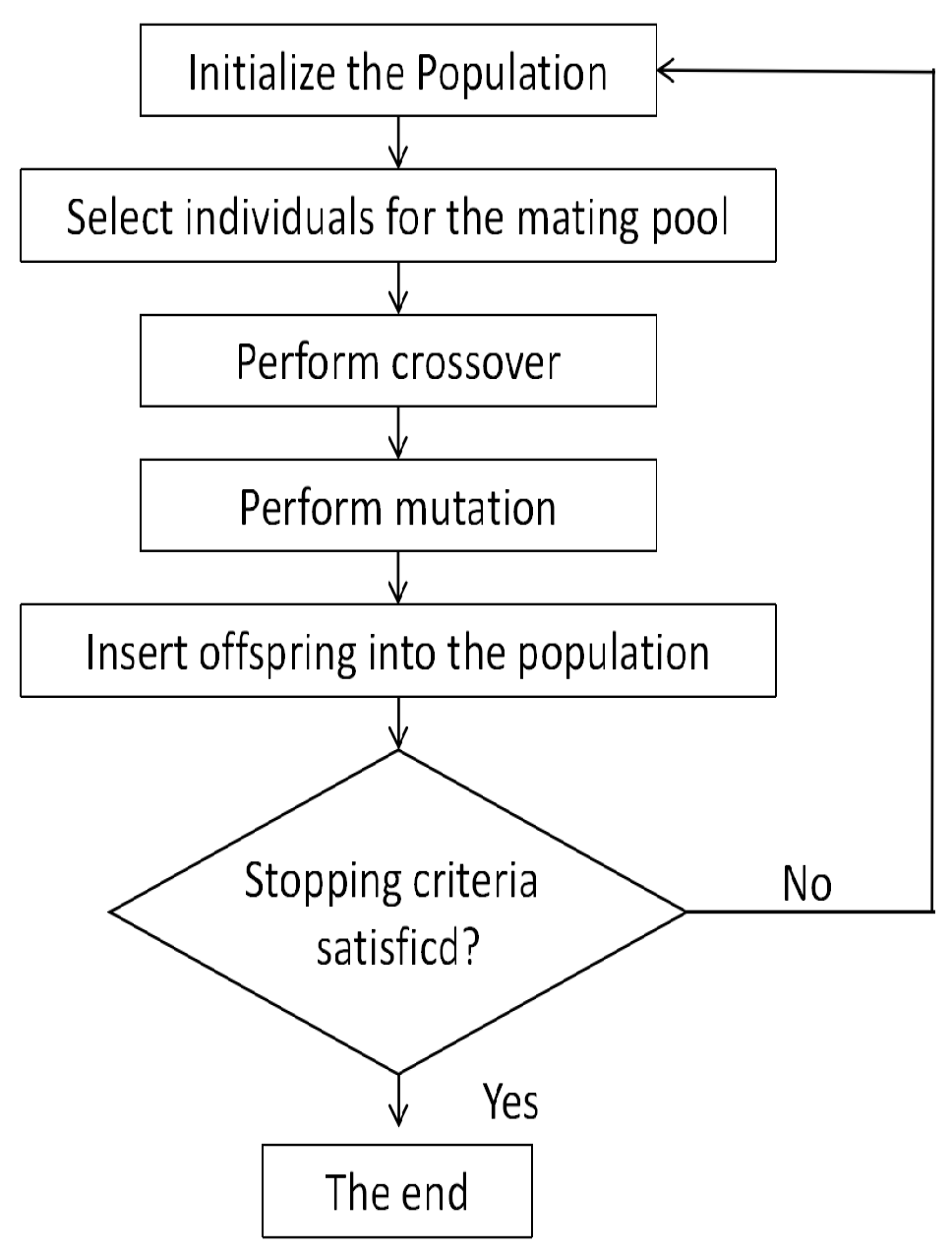
4.2.1. GA

The GA is well suited for addressing production scheduling issues because it operates on a set of potential solutions instead of focusing on a single solution as heuristic searches do. In GA, each chromosome or individual corresponds to a specific sequence of tasks. The algorithm is fundamentally an evolutionary technique that is based on the principle of natural selection, where the fittest survive. The fundamental unit of a GA is the solution encoding, often referred to as a chromosome or an individual, which embodies a potential solution to the problem at hand. Figure 6 depicts the flowchart of the GA process.

(1) Initial solution: The initial solution is obtained randomly as a set of job variations in each machine. The number of operations to perform is equal to the total generations for each chromosome.

(2) Selection: the work is performed using the roulette wheel tournament method.

(3) Crossover: a random procedure is used to cross two points.

(4) Mutation: the exchange mutation is used to avoid the deterioration of the population in its local optimum solution.

(5) Stopping criteria: Generation count is used as a stop condition. In order to solve this problem, we adopt three GA factors, which are population size, crossing probability ($PC$), and mutation probability ($Pm$). Figure 6 illustrates the flow pattern of GA factors.

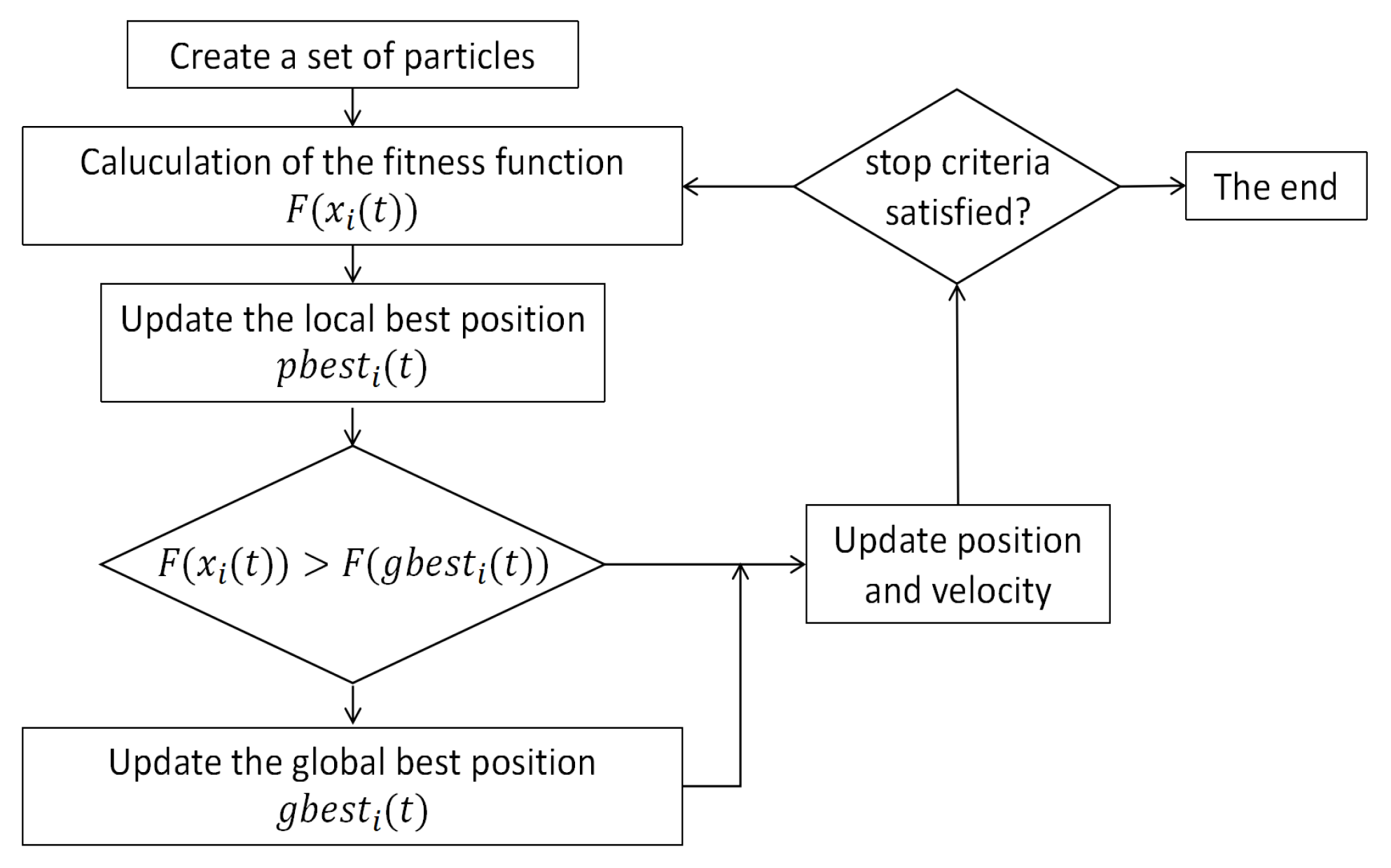
4.2.2. PSO

PSO was developed based on the assumption that birds were social. This paper presents a PSO algorithm that simulates the movement patterns of birds and their information sharing methods to solve an optimization problem. PSO is considered to be one of the most effective algorithms in the real world.

PSO is instrumental in tackling scheduling and routing challenges. The core parameters of PSO include the problem’s dimensionality, the swarm size (number of particles), the inertia weight, the range of iterations, the acceleration constants, and the social cognition factor. Figure 7 shows the operational flow of PSO.

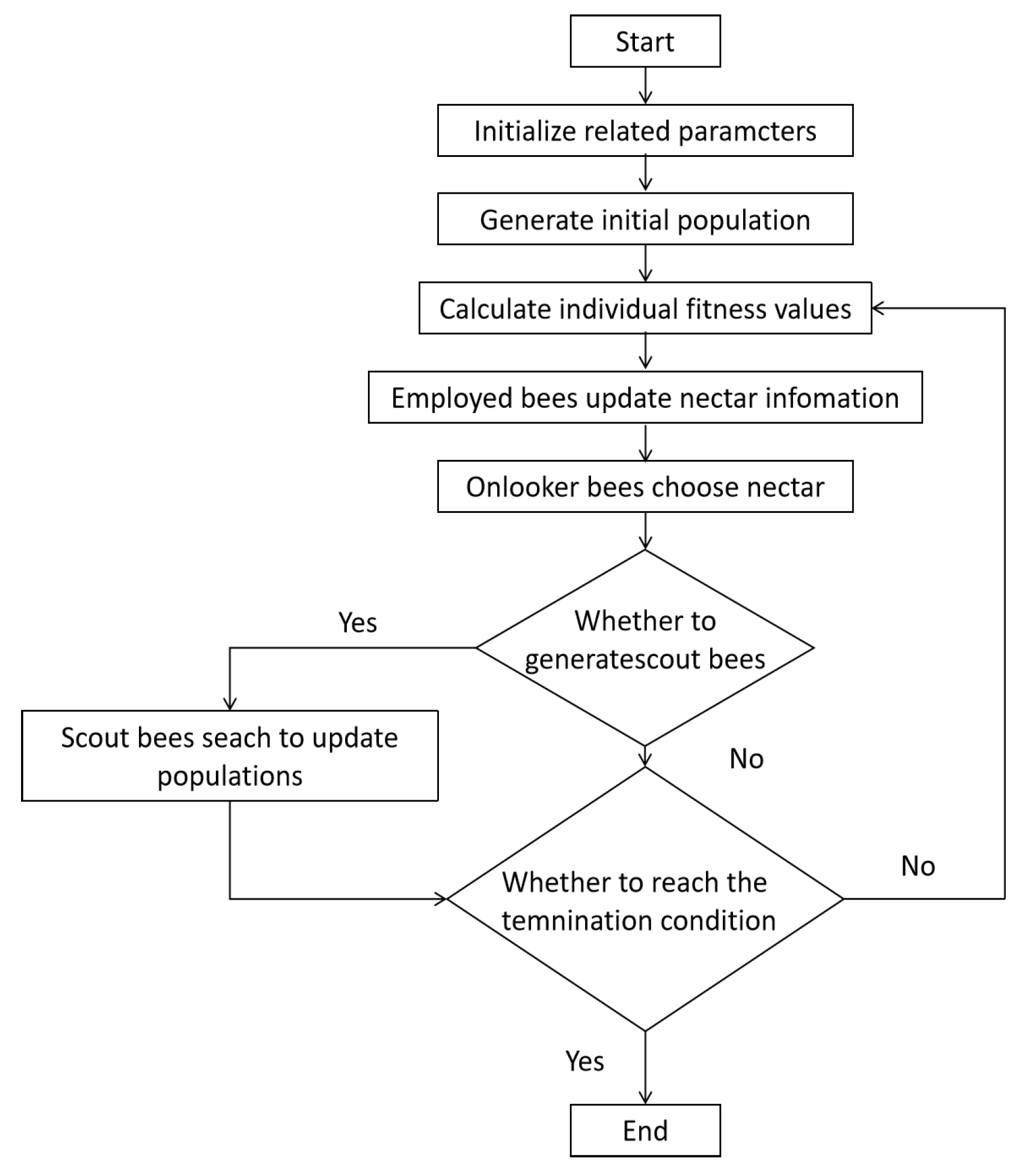
4.2.3. ABC

The problem’s solution space is presumed to be D-dimensional. The count of workers and onlookers is SN, equivalent to the number of nectar sources. The standard ABC algorithm addresses the optimization problem within a 2D search space framework. Each nectar source’s location symbolizes a potential solution, with the number of sources aligning with the fitness of the suitable solution. Employed bees are directly linked to nectar sources. To gain insight into the ABC algorithm, a flowchart is provided. The flowchart of the ABC algorithm is depicted in Figure 8.

4.3. Local Search

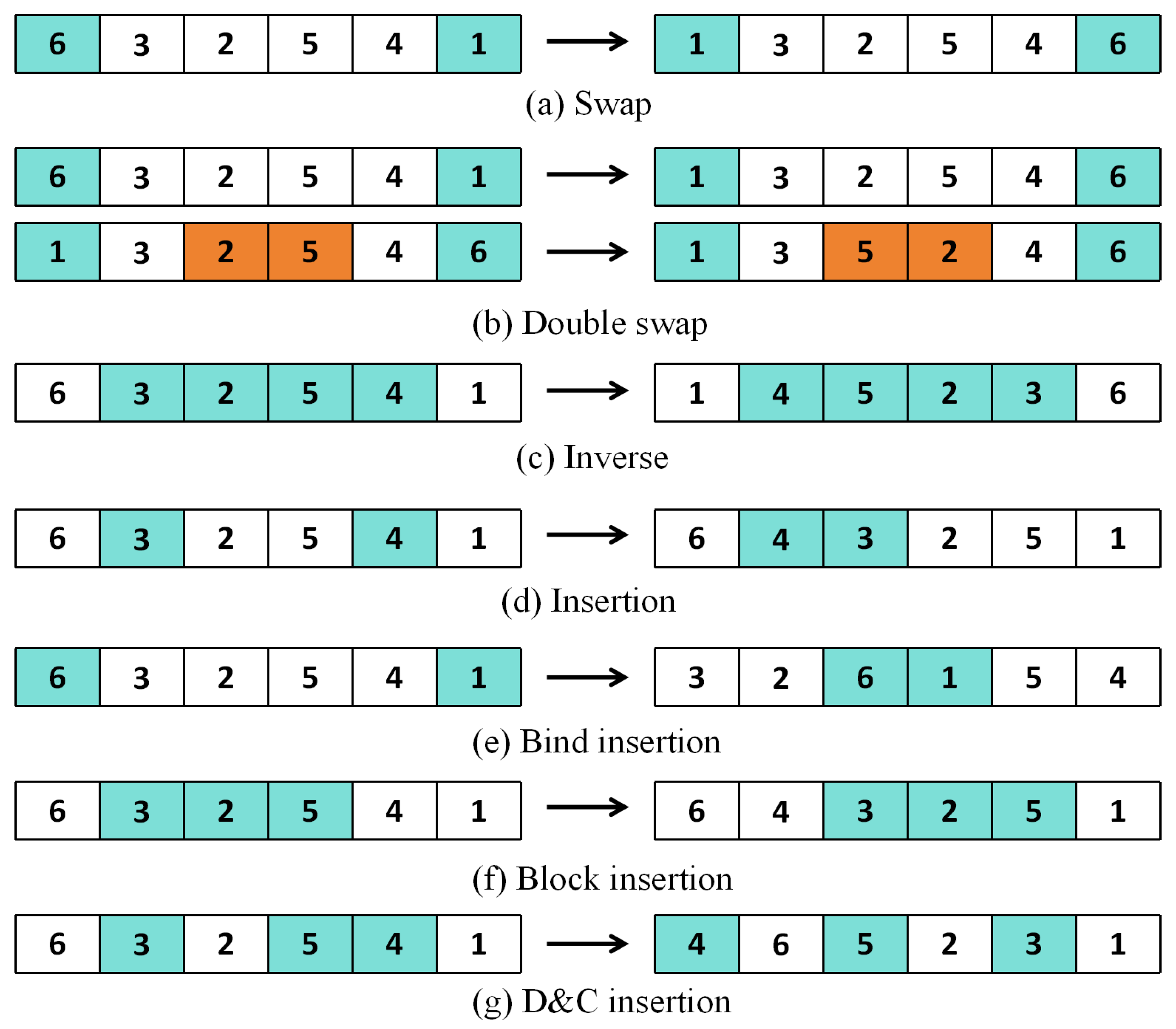
Meta-heuristics are known for their simplicity in implementation and rapid convergence. However, they are prone to falling into local optima during the iterative process. To circumvent settling for a suboptimal solution, this study designs seven local search techniques tailored to the problem’s characteristics. In the BI-JSP-MHR context, we conduct local searches on both the MHR sequences and the job sequence. The details of these seven local search operators are outlined as follows.

(1) Swap: within a solution, two jobs are randomly selected and their positions are interchanged, as shown in Figure 9a.

(2) Double swap: two separate swap operations are performed on a solution, as shown in Figure 9b.

(3) Reverse: two positions are arbitrarily chosen from a solution; reverse all the jobs between the two positions, as depicted in Figure 9c.

(4) Insert: two jobs are randomly chosen, their positional relationship is determined, the second job is inserted into the position of the first, and the subsequent jobs are shifted one position backward, as illustrated in Figure 9d.

(5) Bind insertion: Two jobs are randomly selected and placed in all possible locations while maintaining their order. The process is detailed in Figure 9e.

(6) Block insertion: two different positions within a solution are randomly chosen, treated as a single block, and the block is inserted into all possible locations within the solution, as shown in Figure 9f.

(7) D&C insertion: A set of jobs is randomly extracted from a solution, and these tasks are then randomly inserted back into all potential spots within the solution. Figure 9g shows the arrangement before and after the D&C insertion.

4.4. Reinforcement Learning

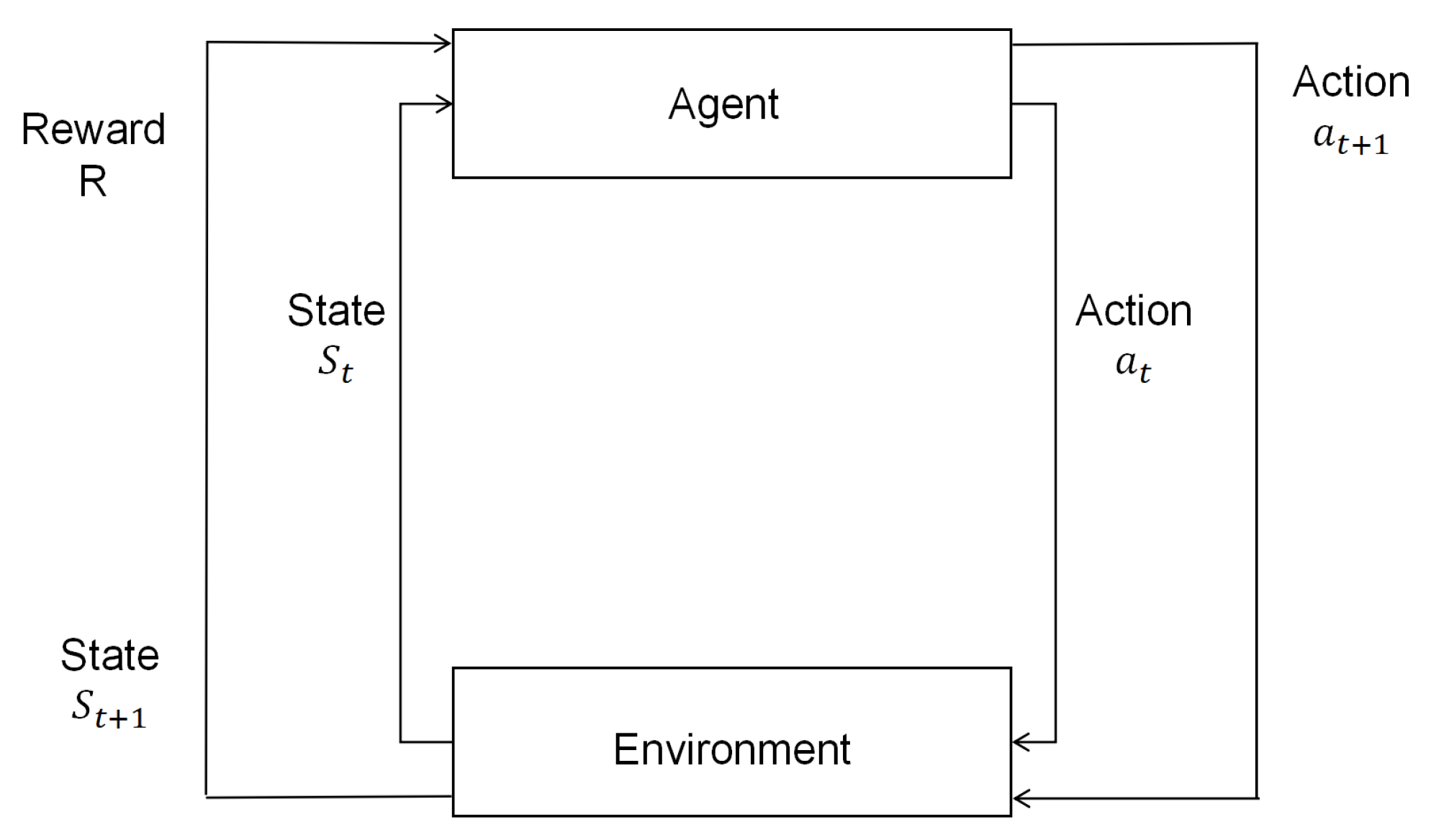
Reinforcement Learning (RL) is a type of machine learning framework in which an intelligent agent learns to make decisions by interacting with its environment to achieve specific goals. Through the process, the agent acquires knowledge and improves its performance over time based on feedback received from the environment. The foundation of RL lies in the ongoing exchange between the agent entities and their environment. Within the dynamic environment, the agent adjustment methods, in accordance with their accumulated experiences, have the objective of amplifying the aggregate value of sustained rewards over an extended period.

Using reinforcement learning to guide the local search process, the algorithm can focus on the most promising regions of the search space and select appropriate local structure. It can also learn to use more efficient search strategies, such as parallel exploration of different regions or adaptive adjustment of the search granularity. It can improve the scalability and efficiency of the algorithm, making it more suitable for solving large-scale and complex optimization problems.

4.4.1. Q-Learning

Q-learning is a decision-making method that does not directly train an agent to choose the correct action. Instead, it evaluates the agent’s actions based on responses from the environment. Through continuous interactions with the environment, agents select actions in response to feedback, with the ultimate goal of making the best decisions. The objective of Q-learning is to identify the Q-value for a specific state-action pair and subsequently determine the optimal action based on these values. Q-values are stored in a Q-table, which is initially a single matrix where the rows correspond to the number of states and the columns correspond to the number of possible actions.

In this study, the concepts of state and action are utilized as components of local search operators within the Q-learning framework. As depicted in Figure 10, the agent selects actions based on the roulette wheel selection approach, which leads to the acquisition of an appropriate reward. Initially, at time t, an agent acquires the current environmental state $s_t$ and performs the action $a_t$. Consequently, the environment transitions to the state $s_{t+1}$, and the agent receives the corresponding reward R. Furthermore, the agent refines its strategy for action selection, enabling the selection of an appropriate action $a_{t+1}$ in subsequent cycles.

At the beginning, the Q-values in the Q-table are initialized to be identical. With each execution of a local search operator by the algorithm, the Q-values in the Q-table are updated. The Q-table itself is refreshed after every iteration. Under certain conditions, Q-learning, being highly probable, can guide the selection of an appropriate local search operator (action). In other words, if an individual performs $L{S}_1$ in state $s_1$, it can select any of the seven local search operators in the next state, which is determined on the basis of Q-values in the Q-table. Thus, Q-learning is designed to assist meta-heuristics in the selection of local search operators. The Q-table appears in

Table 3. Q-table.

LS	a1	a2	a3	a4	a5	a6	a7
s1	Q(s1,a1)	Q(s1,a2)	Q(s1,a3)	Q(s1,a4)	Q(s1,a5)	Q(s1,a6)	Q(s1,a7)
s2	Q(s2,a1)	Q(s2,a2)	Q(s2,a3)	Q(s2,a4)	Q(s2,a5)	Q(s2,a6)	Q(s2,a7)
s3	Q(s3,a1)	Q(s3,a2)	Q(s3,a3)	Q(s3,a4)	Q(s3,a5)	Q(s3,a6)	Q(s3,a7)
s4	Q(s4,a1)	Q(s4,a2)	Q(s4,a3)	Q(s4,a4)	Q(s4,a5)	Q(s4,a6)	Q(s4,a7)
s5	Q(s5,a1)	Q(s5,a2)	Q(s5,a3)	Q(s5,a4)	Q(s5,a5)	Q(s5,a6)	Q(s5,a7)
s6	Q(s6,a1)	Q(s6,a2)	Q(s6,a3)	Q(s6,a4)	Q(s6,a5)	Q(s6,a6)	Q(s6,a7)
s7	Q(s7,a1)	Q(s7,a2)	Q(s7,a3)	Q(s7,a4)	Q(s7,a5)	Q(s7,a6)	Q(s7,a7)

.

The Q-value in the Q-table is updated after an operation is performed. The update formula is as follows:

$$Q\left(s_t,a_t\right)=Q\left(s_t,a_t\right)+\alpha \left[R+\gamma maxQ\left(s_{t+1},a_{t+1}\right)-Q\left(s_t,a_t\right)\right]$$

(17)

In this context, $Q(s_t,a_t)$ represents the Q-value associated with performing an action $a_t$ in the present state $s_t$. The parameter $\alpha$ denotes the learning rate, R signifies the reward received, $\gamma$ is the discount factor, and $maxQ(s_{t+1},a_{t+1})$ refers to the maximum Q-value that can be obtained by selecting an action $a_{t+1}$ in the next state $s_{t+1}$ using a roulette wheel selection method. The expression for R is given by

$$R=\left\{\begin{array}{c}\left(C_{max}-C_{max}^{\prime }\right)\times 2+\left(E/T-{E/T}^{\prime }\right)\times 2,C_{max}>C_{max}^{\prime }andE/T>{E/T}^{\prime }\\ 2,C_{max}>C_{max}^{\prime }andE/T={E/T}^{\prime }or{C}_{max}=C_{max}^{\prime }andE/T>{E/T}^{\prime }\\ 1,C_{max}>C_{max}^{\prime }andE/T<{E/T}^{\prime }or{C}_{max}<C_{max}^{\prime }andE/T>{E/T}^{\prime }\\ 0,C_{max}<C_{max}^{\prime }andE/T<{E/T}^{\prime }or{C}_{max}<C_{max}^{\prime }andE/T<{E/T}^{\prime }\end{array}\right.$$

(18)

where $C_{max}^{\prime }$, $E/T^{\prime }$ are the makespan and E/T of the new solution while the $C_{max}$ and $E/T$ are the old one.

4.4.2. SARSA

Unlike Q-Learning, SARSA is a web-based online learning algorithm. If the Q function is updated, it uses the action value of the following action $a^{\prime }$ that the agent actually receives: $Q_t(s^{\prime },a^{\prime })$. It means that SARSA takes into account the agent’s existing policy throughout the learning process. Therefore, the policy that SARSA has learned has a close relationship with the practice of the agent in the course of training.

The main difference between Q-learning and SARSA is the update strategy for Q-values. In Q-learning, the expected maximum Q-value obtained by all possible actions in the next state is selected as a factor to update the Q-value under the current state. However, the action with the expected maximum value may not necessarily be executed in the next state. In SARSA, a Q-value obtained by an action in the next state is also used to update the current Q-value, and the action is executed in the next state.

The SARSA algorithm updates the estimation of the value function in every strategy step.The agent operates based on the $\epsilon -greedy$ approach. It only needs to know the state of the preceding step ($s_t$), the prior action ($a_t$), the reward value (R), the present state ($s_t^{\prime }$), and the action ($a_t^{\prime }$). The formula for updating the action value function is given in the equation below. $Q(s,a)$ is used as the Q-value for the states to perform the action a, $\alpha$ is the learning rate, and $\gamma$ is the discount factor.

$$Q\left(s_t,a_t\right)=Q\left(s_t,a_t\right)+\alpha \left[R+\gamma Q\left(s_{t+1},a_{t+1}\right)-Q\left(s_t,a_t\right)\right]$$

(19)

Despite differences in action selection and Q-value update methodologies, there are similarities between SARSA and Q-learning in various aspects of their learning processes. Both algorithms initialize the Q-table with arbitrary values, typically zeros, and update their Q-value using equivalent reward values. Moreover, the objective of these two algorithms is to learn an optimal strategy that maximizes the cumulative reward.

In summary, SARSA introduces a more exploratory approach to action selection than Q-learning, which uses existing policies to decide what to do in the update. This may result in better environmental research and, in certain cases, quicker convergence towards optimum policies.

4.5. The Framework of Proposed Algorithms

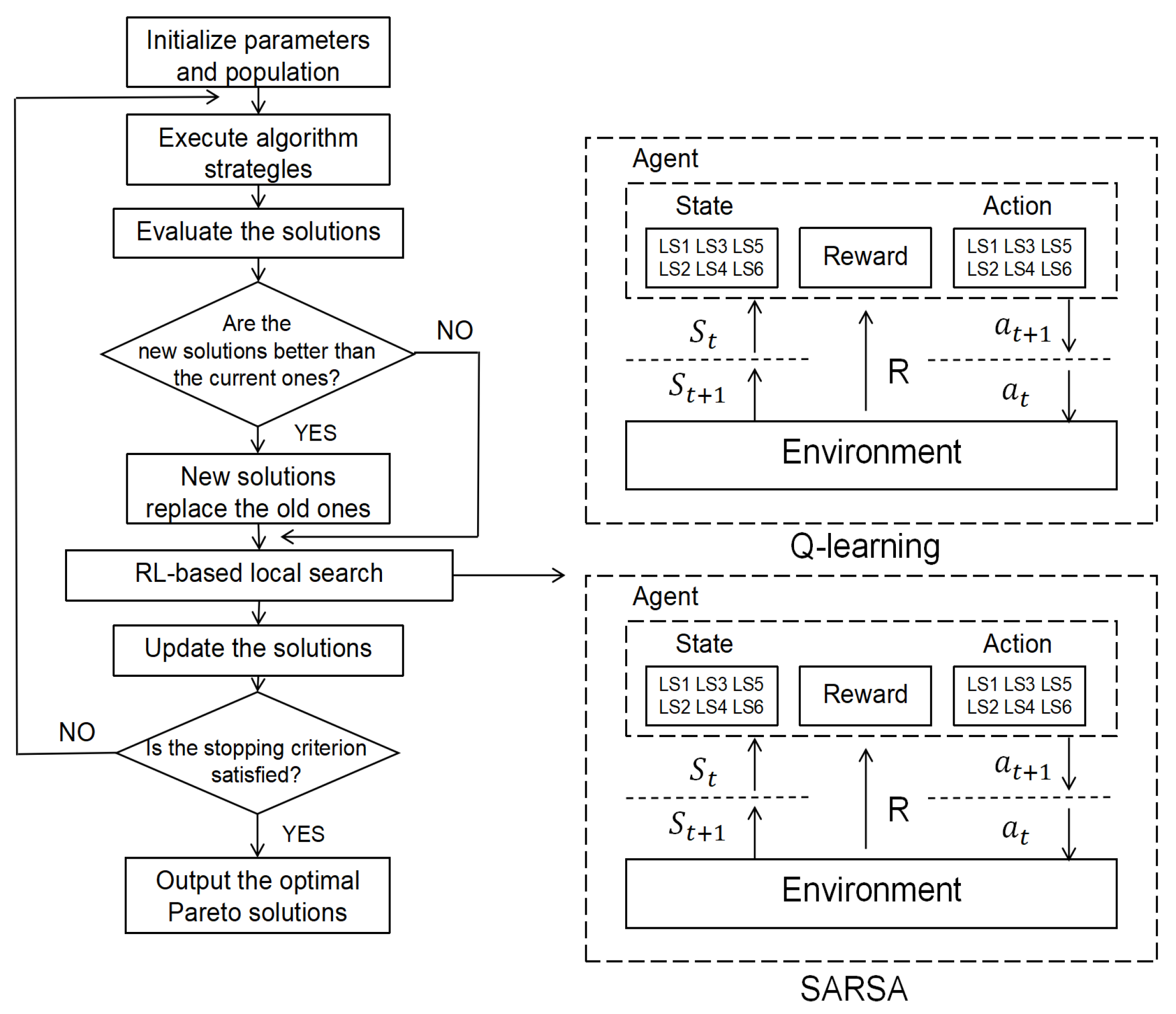
This work designs three enhanced meta-heuristics with Q-learning and SARSA. Figure 11 illustrates the architecture of the Q-learning and SARSA process. Initially, parameters and the population are established. Then, a novel solution is generated through a unique algorithmic approach. After that, the population is adjusted based on the newly generated solution. Next, a local search operator is determined using Q-learning or SARSA. If the Q-learning or SARSA strategy obtains a solution with better performance, it means that the chosen action (e.g., local search operator) is more conducive to maximizing the cumulative reward. Subsequently, the Q-values in the Q-table are updated. The larger the Q-value, the higher the probability that a local search operator will be selected in subsequent iterations. In conclusion, these steps are repeated in a loop until a predefined stopping criterion is met. At that point, the result of the process is reported as the final outcome.

5. Experiments and Discussions

5.1. Experimental Setup

To evaluate the performance of our method, we generate 82 extensive benchmark cases from [55]. These cases encompass combinations of the number of jobs n in $\{6,10,15,50\}$, the number of machines m in $\{5,6,10,15,20\}$, and Number of MHRs v in $\{3,4,5,6\}$. The setup time of the cases is generated within the range of 1 to 10 under a normal distribution. We adopt the strategy from Ciholami [56] to incorporate relevant data into our datasets. The deadline is calculated using the following formula:

$$D_i=\left(1+{\displaystyle \frac{T\times n}{m}}\right)\times \sum _{j=1}^{n_i}{P}_{i,j}$$

T is a constant, specifically $T=0.3$ [57], n represents the number of jobs, m denotes the number of machines, and $P_{i,j}$ is the mean processing time of all selected machines.

The algorithms under comparison are implemented in Python and executed on a system furnished with a 13th Gen Intel® Core™ i7-13700K CPU(Intel, Santa Clara, CA, USA) @ 3.40GHz and 64.0 GB of RAM, running Microsoft Windows 11 Pro for Workstations. For the fairness of the experiments, all instances are run in the same environment, and each algorithm is run independently 20 times for a case. The time limit for each run is set to $t=0.3\times m\times n\times v$ seconds, with a population size set at 5.

To assess the effectiveness of multi-objective optimization algorithms, we employ two metrics: $\rho$ [58] and the Inverse Generational Distance (IGD) [59]. The metric $\rho$ is utilized to evaluate the solution quality, while IGD measures the convergence and diversity of the algorithms. A higher $\rho$ value indicates superior algorithmic performance, and a lower IGD value implies a more competitive algorithm.

The $\rho$ metric is calculated as the proportion of elements in the set $\left\{x\in PS|x\in PF\right\}$ to $PF$. Here, $PS$ represents the Pareto non-dominated solutions obtained by an algorithm, and $PF$ denotes the approximate Pareto front. It is crucial to understand that the true Pareto front is typically unknown in practical scenarios. For this study, we consider the Pareto non-dominated solutions from all contrasted algorithms that constitute the approximate Pareto front.

The metric IGD can be computed as

$$IGD\left(P_S,P_F\right)={\displaystyle \frac{1}{\left|P_F\right|}}\sum _{V\in P_F}d(v,z)$$

where $d(v,z)$ denotes the gap between the solution v and the reference point z. The notation $\left|PF\right|$ refers to the count of solution instances that are spread across the Pareto front $PF$.

5.2. Parameter Setting

The settings of the parameters for an algorithm can significantly influence its effectiveness. The parameters are set based on our previous research and compared algorithms [48]. Taking the case of the instance “20_20”, we assess the advantages and disadvantages of diverse parameter arrangements for all compared algorithms. Each parameter setup is run separately for 20 times, with the IGD metric serving as the outcome measure, which IGD typically gauges the convergence and diversity of the algorithms’ values. A smaller IGD value generally suggests a more formidable algorithm, often reflecting a higher quality collection of solutions.

In the ABC. The ABC algorithm involves three key parameters: Employed Bees ($EP$), Onlooker Bees ($OP$), and Scout Bees ($SP$). Drawing on previous studies, we set the ratios of $EP$ and $SP$: $EP$ in $\{0.4,0.5,0.6,0.7\}$ and $SP$ in $\{0.1,0.2,0.3\}$. $OP$ can be calculated as $1-EP-SP$. Using the trend of parameters depicted in Figure 12, we set the parameters for ABC, where $EP=0.6$, $OP=0.2$, and $SP=0.2$.

In the PSO, three crucial parameters need consideration: the inertia weight (W), the personal cognition coefficient ($C1$), and the social cognition coefficient ($C2$). The possible values for these parameters are W in $\{0.2,0.4,0.6,0.8\}$, $C1$ in $\{1,2,3,4\}$, and $C2$ in $\{1,2,3,4\}$. Analyzing the graph presented in Figure 13, we determine the optimal values for W, $C1$, and $C2$ to be 0.6, 3, and 3, respectively.

The performance of the GA is largely affected by the crossover probability ($PC$) and mutation probability ($Pm$). Consequently, we conduct a parameter tuning experiment for these two parameters, $PC$ ranging in $\{0.6,0.7,0.8,0.9,1\}$ and $Pm$ ranging in $\{0.2,0.4,0.6,0.8,1\}$. Figure 14 indicates that the algorithm achieves optimal performance when $PC$ is set to 0.7 and $Pm$ is set to 0.8.

Additionally, for Q-learning and SARSA, we focus on two key parameters: the learning rate $\alpha$ and the discount rate $\gamma$. The values for $\alpha$ are considered within $\{0.6,0.7,0.8,0.9\}$ and for $\gamma$ within $\{0.1,0.2,0.3,0.4\}$. Given that GA_Q and GA_S have demonstrated superior performance in addressing similar problems, we fine-tune $\alpha$ and $\gamma$ in Q-learning based on the average performance metrics obtained from GA_Q and GA_S. Analyzing Figure 15 and Figure 16, we determine the optimal settings for $\alpha$ and $\gamma$ to be 0.7 and 0.2, respectively.

5.3. Results and Comparisons

5.3.1. Within-Group Comparisons of the Developed Methods

The efficacy of the proposed local search operators, Q-learning, and SARSA are confirmed through testing. We compare three meta-heuristic algorithms: GA, PSO, and ABCm with their variants with local search operators (GA_L, PSO_L, ABC_L), variants with Q-learning (GA_Q, PSO_Q, ABC_Q), and variants with SARSA-based local search operators (GA_S, PSO_S, ABC_S). Variants with local search operators refer to algorithms that randomly select local search operators during each iteration.

Table 4. IGD statistics results for GA and its variants.

	GA	GA_L	GA_Q	GA_S		GA	GA_L	GA_Q	GA_S
abz5	147.72	23.75	70.01	150.03	la34	755.15	213.75	175.71	0
abz6	178.9	58.37	0	71.82	la35	725.96	152.43	155.59	0
abz7	538.15	323.68	260.39	0	la36	525.89	143.76	151.32	0
abz8	516.83	202.76	131.04	0	la37	657.12	392.05	271.54	0
abz9	486.16	241.44	157.19	0	la38	514.69	200.86	149.68	0
ft06	37.77	3.92	43.38	55.25	la39	546.54	214.8	206.18	0
ft10	355.54	121.33	129.16	0	la40	673.66	306.23	274.15	0
ft20	284.42	31.75	69.79	31.75	orb01	316.31	98.65	66.27	0
la01	81	19.16	18.14	12.83	orb02	333.08	186.63	127.17	0
la02	93.12	27.67	3.82	6.94	orb03	276.57	25.59	40.12	27.84
la03	113.06	20.16	22.15	6.34	orb04	138.36	8.36	14.14	45.68
la04	45.52	0	17.15	26.78	orb05	336.48	171.56	90.01	0
la05	61.82	10.6	21.62	23.88	orb06	172.42	34.76	33.62	10.32
la06	82.99	48.44	19.67	6.43	orb07	300.08	113.47	145.77	0
la07	124.82	3.43	18.93	19.15	orb08	247.56	32.63	98.98	2.3
la08	130.94	72.72	58.7	0	orb09	132.32	37.77	34.16	33.05
la09	186.05	70.52	53.96	0	orb10	278.71	130.81	49.07	0
la10	141.68	65.3	19.48	0	swv01	659.8	185.13	236.78	0
la11	244.13	72.16	72.21	0	swv02	638.47	195.77	181.62	0
la12	215.28	59.67	45.44	0	swv03	623.95	14.98	22.06	31.54
la13	183.19	58.09	55.22	0	swv04	727.54	191.17	164.39	0
la14	153.56	50.1	46.71	0	swv05	639.67	142.15	93.38	0
la15	143.59	28.38	29.62	0	swv06	1104.3	473.09	350.89	0
la16	328.18	131.29	107.69	0	swv07	1050.05	338.08	278.38	0
la17	297.41	65.12	64.35	0	swv08	1109.45	367.4	195.16	0
la18	444.15	183.51	238.03	0	swv09	817.02	209.32	154.38	0
la19	243.86	16.97	11.57	8.75	swv10	1030.09	382.43	336.76	0
la20	311.92	72.93	82.53	0	swv11	1494.11	51.66	81.62	82.02
la21	393.95	121.26	80.47	0	swv12	1490.96	325.78	308.27	0
la22	414.8	87.21	23.68	1.25	swv13	1948.77	446.83	370.11	0
la23	300.65	70.66	0	82.33	swv14	1505.27	381.14	277.25	0
la24	328.62	37.56	0	113.35	swv15	1847.38	645.67	453.5	0
la25	381.66	149.85	103.87	0	swv16	1384.62	428.09	383.54	0
la26	389.63	53.07	85.53	0	swv17	1295.19	438.06	255.52	0
la27	624.76	188.63	69.37	0	swv18	1116.51	506.38	471.55	0
la28	526.4	209.7	151.67	0	swv19	1139.02	439.61	348.07	0
la29	627.13	225.71	283.07	0	swv20	1157.33	323.84	372.97	0
la30	585.38	160.88	204.63	0	yn1	710.56	348.32	315.43	0
la31	767.54	208.56	178.58	0	yn2	666.05	344.7	200.82	0
la32	814.13	307.07	151.98	0	yn3	605.92	316.39	282.71	0
la33	769.84	128.52	38.49	19.31	yn4	868.03	454.21	346.74	0

,

Table 5. IGD statistics results for PSO and its variants.

	PSO	PSO_L	PSO_Q	PSO_S		PSO	PSO_L	PSO_Q	PSO_S
abz5	735.28	76.49	21.93	12.48	la34	1088.31	59.71	14.2	30.72
abz6	680.59	142.92	39.22	0	la35	1027.17	68.76	42.14	5.22
abz7	989.29	191.87	227.97	0	la36	1002.37	42.33	0	148.83
abz8	769.32	57.57	51.94	25.2	la37	1331.35	303.87	252.26	0
abz9	909	110.98	0	115.48	la38	1202.26	195.27	225.37	0
ft06	62.93	0	19.11	51.34	la39	982.25	35.86	106.8	0
ft10	699.2	196.01	73.83	22.55	la40	1276.15	237.3	268.54	0
ft20	455.12	61.95	54.63	0	orb01	704.84	78.79	156.43	0
la01	186	2.93	28.93	15.99	orb02	653.98	166.7	165.9	0
la02	170.15	12.51	12.92	10.3	orb03	603.17	26.48	22.32	55.32
la03	183.66	5.26	10.53	14.33	orb04	615.33	52.84	142.95	0
la04	255.3	0	86.15	84.42	orb05	544.89	0	94.85	57.77
la05	133.48	4.85	14.58	8.29	orb06	685.41	230.46	237.52	0
la06	259.97	67.06	39	0	orb07	632.79	126.28	143.47	0
la07	356.05	61.11	76.26	0	orb08	681.69	284.13	237.43	0
la08	266.97	0	29.75	42.41	orb09	538.81	67.78	118	2.54
la09	314.65	0	61.48	18.57	orb10	634.68	109.92	0	91.29
la10	273.42	64.64	42.56	12.71	swv01	745.29	10.46	32.94	43.39
la11	344.01	0	55.91	41.02	swv02	983.67	218.76	236.64	0
la12	347.19	38.29	50.82	0.18	swv03	918.25	211.75	255.86	0
la13	441.02	21.57	59.93	8.43	swv04	1079.56	74.52	197.71	0
la14	417.24	29.82	41.86	29.82	swv05	1060.32	321.76	256.18	0
la15	400.95	24.92	64.14	25.19	swv06	1439.56	276.08	196.39	0
la16	607.37	127.45	17.08	0	swv07	1302.06	118.08	142.02	0
la17	600.97	117.27	106.68	0	swv08	1107.39	0	33.13	467
la18	585.48	110.64	76.03	0	swv09	1571.65	300.39	368.26	0
la19	453.78	20.86	29.88	42.68	swv10	1279.73	0	241.3	273.15
la20	693.76	165.52	151.85	0	swv11	1501.17	0	145.64	351.78
la21	546.65	23.94	76.94	0	swv12	1924.92	261.65	207.74	0
la22	673.06	0	172.45	70.8	swv13	1940.12	0	320.61	116.86
la23	663.78	114.15	104.18	0	swv14	1766.54	0	231	277.37
la24	728.82	215.68	171.15	0	swv15	1745.34	0	176.54	329.04
la25	666.12	146.04	69.93	22.74	swv16	1805.81	451.2	398.64	0
la26	842.95	69.24	92.01	0	swv17	1543.09	33.63	70.3	23.21
la27	1006.22	251.72	202.56	0	swv18	1391.1	14.97	14.97	111.67
la28	983.64	173.28	244.54	0	swv19	1927.8	612.32	536.94	0
la29	941.88	143.52	107.65	0	swv20	1864.4	449.45	421.7	0
la30	916.5	248.41	155.21	0	yn1	1448.87	98.32	203.41	0
la31	1052.93	72.86	59.61	12.5	yn2	1389.71	315.23	273.07	0
la32	1217.13	204.39	215.07	0	yn3	1300.86	28.18	0	90.17
la33	1139.49	98.12	0	77.23	yn4	1301.79	73.37	116.65	0

,

Table 6. IGD statistics results for ABC and its variants.

	ABC	ABC_L	ABC_Q	ABC_S		ABC	ABC_L	ABC_Q	ABC_S
abz5	824.25	0	69.17	164.27	la34	1065.36	0	118.72	251.4
abz6	767.1	85.05	158.52	0	la35	1381.84	265.74	266.85	0
abz7	908.43	236.69	152.01	0	la36	1294.68	179.81	186.38	0
abz8	949.57	0	106.53	190.63	la37	1244.43	56.75	114.11	0
abz9	898.92	67.59	66.84	31.03	la38	1183.16	75.84	48.97	17.81
ft06	125.64	37.64	38.73	0	la39	1191.42	98.63	0	87.28
ft10	570.49	43.27	85.45	0	la40	1361.61	213.34	232.78	0
ft20	341.79	54.92	32.57	34.3	orb01	624.15	27.48	47.18	130.34
la01	223.66	9.3	14.06	26.91	orb02	533.53	14.17	65.78	97.83
la02	141	43.35	13.44	34.06	orb03	557.16	62.24	9.2	32.34
la03	235.67	19.08	27.02	0	orb04	608.83	3.28	85.51	16.88
la04	249.15	23.23	8.23	20.89	orb05	717.11	55.23	66.59	132.19
la05	264.19	61.41	25.62	0	orb06	717.86	0	97.31	90.09
la06	248.94	20.38	74.46	72.86	orb07	636.6	75.71	68.27	0
la07	310.97	69.95	85.38	0	orb08	727.44	42.01	143.75	0
la08	300.32	46.45	10.48	20.94	orb09	671.37	74.06	0	183.67
la09	307.78	8.12	18.79	32.09	orb10	861.03	151.13	247	0
la10	377.49	37.26	40.15	7.91	swv01	853.22	74.76	117.14	8.19
la11	409.9	70.92	26.03	3.44	swv02	819.39	27.67	106.88	83.99
la12	414.14	48.96	71.2	0	swv03	914.84	141.51	87.51	20.04
la13	301.7	25.27	19.27	38.4	swv04	1002.65	135.93	283.65	0
la14	383.15	38.57	2.13	32.37	swv05	935.19	19.48	75.36	70.76
la15	390.37	13.96	26.84	13	swv06	1339.24	230.65	160.46	0
la16	444.43	28.97	0.93	114	swv07	1356.78	155.92	37.96	0
la17	619.49	62.23	70.73	0	swv08	1363.43	41.87	99.83	0
la18	605.23	123.69	206.15	0	swv09	990.69	8.57	77.13	159.79
la19	657.77	23.76	10.33	39.48	swv10	1356.43	171.02	170.97	0
la20	497.11	6.79	8.96	44.51	swv11	1773.39	135.59	406.47	48.37
la21	692.66	10.33	38.26	27.55	swv12	1583.19	32.16	58.15	193.12
la22	867.36	104.7	181.46	0	swv13	1828.81	239.52	323.52	0
la23	870.19	167.54	237.33	0	swv14	1744.14	129.18	138.67	0
la24	965.26	251.08	218.88	0	swv15	1882.24	330.48	431.01	0
la25	681.63	32.88	20.2	6.96	swv16	1621.61	0	141.96	314.24
la26	906.98	36.17	154.85	17.67	swv17	2146.63	503.39	447.73	0
la27	892.8	157.76	99.49	0	swv18	1875.72	101.28	263.06	0
la28	941.57	10.55	10.55	48.67	swv19	1540.95	165.64	25.63	187.65
la29	870.6	65.81	22.11	22.11	swv20	1718.84	18.12	80.34	56.32
la30	978.51	29.95	15.73	21.51	yn1	1169.4	0	60.7	293.64
la31	1026.3	57.54	27.2	30.9	yn2	1320.25	87.01	147.33	0
la32	1416.65	233.77	198.29	0	yn3	1313.44	140.81	38.39	35.01
la33	1126.26	68.2	76.1	12.02	yn4	1474.65	193.64	193.89	0

,

Table 7. $\rho$ statistics results for GA and its variants.

	GA	GA_L	GA_Q	GA_S		GA	GA_L	GA_Q	GA_S
abz5	0	0.5	0.5	0	la34	0	0	0	1
abz6	0	0	1	0	la35	0	0	0	1
abz7	0	0	0	1	la36	0	0	0	1
abz8	0	0	0	1	la37	0	0	0	1
abz9	0	0	0	1	la38	0	0	0	1
ft06	0	0.8	0	0.2	la39	0	0	0	1
ft10	0	0	0	1	la40	0	0	0	1
ft20	0	0.5	0	0.5	orb01	0	0	0	1
la01	0	0.4	0.2	0.4	orb02	0	0	0	1
la02	0	0	0.67	0.33	orb03	0	0.5	0.25	0.25
la03	0	0.25	0	0.75	orb04	0	0.5	0.5	0
la04	0	1	0	0	orb05	0	0	0	1
la05	0	0.5	0.25	0.25	orb06	0	0	0.33	0.67
la06	0	0	0.4	0.6	orb07	0	0	0	1
la07	0	0.75	0.25	0	orb08	0	0.14	0	0.86
la08	0	0	0	1	orb09	0	0.4	0.2	0.4
la09	0	0	0	1	orb10	0	0	0	1
la10	0	0	0	1	swv01	0	0	0	1
la11	0	0	0	1	swv02	0	0	0	1
la12	0	0	0	1	swv03	0	0.4	0.2	0.4
la13	0	0	0	1	swv04	0	0	0	1
la14	0	0	0	1	swv05	0	0	0	1
la15	0	0	0	1	swv06	0	0	0	1
la16	0	0	0	1	swv07	0	0	0	1
la17	0	0	0	1	swv08	0	0	0	1
la18	0	0	0	1	swv09	0	0	0	1
la19	0	0	0.5	0.5	swv10	0	0	0	1
la20	0	0	0	1	swv11	0	0.33	0.33	0.33
la21	0	0	0	1	swv12	0	0	0	1
la22	0	0	0.25	0.75	swv13	0	0	0	1
la23	0	0	1	0	swv14	0	0	0	1
la24	0	0	1	0	swv15	0	0	0	1
la25	0	0	0	1	swv16	0	0	0	1
la26	0	0	0	1	swv17	0	0	0	1
la27	0	0	0	1	swv18	0	0	0	1
la28	0	0	0	1	swv19	0	0	0	1
la29	0	0	0	1	swv20	0	0	0	1
la30	0	0	0	1	yn1	0	0	0	1
la31	0	0	0	1	yn2	0	0	0	1
la32	0	0	0	1	yn3	0	0	0	1
la33	0	0	0.33	0.67	yn4	0	0	0	1

,

Table 8. $\rho$ statistics results for PSO and its variants.

	PSO	PSO_L	PSO_Q	PSO_S		PSO	PSO_L	PSO_Q	PSO_S
abz5	0	0	0.333	0.167	la34	0	0	0.667	0.333
abz6	0	0	0	0.444	la35	0	0	0.25	0.75
abz7	0	0	0	0.667	la36	0	0	0.5	0
abz8	0	0	0.333	0.667	la37	0	0	0	0.75
abz9	0	0	1	0	la38	0	0	0	1
ft06	0	0.364	0	0	la39	0	0	0	0.333
ft10	0	0	0.25	0.5	la40	0	0	0	0.667
ft20	0	0	0	0.6	orb01	0	0	0	0.333
la01	0	0.143	0	0.143	orb02	0	0	0	0.667
la02	0	0.1	0.1	0.3	orb03	0	0.5	0.5	0
la03	0	0.333	0.333	0	orb04	0	0	0	1
la04	0	1	0	0	orb05	0	1	0	0
la05	0	0.375	0.125	0.25	orb06	0	0	0	1
la06	0	0	0	0.5	orb07	0	0	0	0.833
la07	0	0	0	1	orb08	0	0	0	1
la08	0	0.833	0	0	orb09	0	0.048	0	0.143
la09	0	1	0	0	orb10	0	0	0.5	0
la10	0	0	0.25	0.5	swv01	0	0.667	0.333	0
la11	0	0.75	0	0	swv02	0	0	0	0.667
la12	0	0.043	0	0.304	swv03	0	0	0	1
la13	0	0.2	0	0.4	swv04	0	0	0	1
la14	0	0.5	0	0.5	swv05	0	0	0	1
la15	0	0.333	0	0.667	swv06	0	0	0	0.667
la16	0	0	0	0.167	swv07	0	0	0	1
la17	0	0	0	0.375	swv08	0	0.8	0	0
la18	0	0	0	0.5	swv09	0	0	0	0.556
la19	0	0.333	0.333	0.167	swv10	0	1	0	0
la20	0	0	0	1	swv11	0	0.5	0	0
la21	0	0	0	0.667	swv12	0	0	0	0.25
la22	0	1	0	0	swv13	0	1	0	0
la23	0	0	0	0.6	swv14	0	1	0	0
la24	0	0	0	1	swv15	0	1	0	0
la25	0	0	0.25	0.5	swv16	0	0	0	1
la26	0	0	0	1	swv17	0	0.333	0	0.333
la27	0	0	0	1	swv18	0	0.5	0.5	0
la28	0	0	0	1	swv19	0	0	0	1
la29	0	0	0	1	swv20	0	0	0	0.5
la30	0	0	0	0.6	yn1	0	0	0	0.571
la31	0	0	0.2	0.6	yn2	0	0	0	1
la32	0	0	0	0.8	yn3	0	0	1	0
la33	0	0	1	0	yn4	0	0	0	0.6

and

Table 9. $\rho$ statistics results for ABC and its variants.

	ABC	ABC_L	ABC_Q	ABC_S		ABC	ABC_L	ABC_Q	ABC_S
abz5	0	1	0	0	la34	0	0.5	0	0
abz6	0	0	0	1	la35	0	0	0	1
abz7	0	0	0	1	la36	0	0	0	0.67
abz8	0	0.5	0	0	la37	0	0	0	1
abz9	0	0.17	0.17	0.17	la38	0	0	0.33	0.33
ft06	0	0	0	0.17	la39	0	0	1	0
ft10	0	0	0	0.67	la40	0	0	0	0.5
ft20	0	0	0.5	0.5	orb01	0	0.44	0.11	0.33
la01	0	0.67	0.17	0.17	orb02	0	0.67	0.33	0
la02	0	0.33	0.11	0	orb03	0	0.13	0.38	0.13
la03	0	0	0	1	orb04	0	0.2	0	0.2
la04	0	0	0.75	0.25	orb05	0	0.5	0.5	0
la05	0	0	0	1	orb06	0	0.29	0	0
la06	0	0.33	0.33	0.33	orb07	0	0	0	1
la07	0	0	0	0.83	orb08	0	0	0	1
la08	0	0.14	0.43	0.29	orb09	0	0	0.5	0
la09	0	0.6	0.2	0	orb10	0	0	0	1
la10	0	0.13	0.13	0.38	swv01	0	0.17	0	0.83
la11	0	0	0.25	0.25	swv02	0	0.5	0.25	0.25
la12	0	0	0	0.5	swv03	0	0	0.14	0.43
la13	0	0.33	0.33	0.33	swv04	0	0	0	0.67
la14	0	0.09	0.45	0.09	swv05	0	0.67	0	0.17
la15	0	0.21	0	0.21	swv06	0	0	0	0.67
la16	0	0.09	0.27	0	swv07	0	0	0	1
la17	0	0	0	1	swv08	0	0	0	0.5
la18	0	0	0	0.6	swv09	0	0.67	0.17	0
la19	0	0.33	0.67	0	swv10	0	0	0	1
la20	0	0.33	0.22	0	swv11	0	0.33	0	0.67
la21	0	0.33	0.33	0.17	swv12	0	0.43	0.29	0
la22	0	0	0	1	swv13	0	0	0	1
la23	0	0	0	0.67	swv14	0	0	0	1
la24	0	0	0	0.23	swv15	0	0	0	1
la25	0	0	0.33	0.67	swv16	0	1	0	0
la26	0	0.33	0	0.67	swv17	0	0	0	1
la27	0	0	0	1	swv18	0	0	0	1
la28	0	0.5	0.5	0	swv19	0	0.29	0.43	0.14
la29	0	0	0.5	0.5	swv20	0	0.67	0	0.33
la30	0	0	0.67	0.33	yn1	0	0.75	0	0
la31	0	0.2	0.2	0.6	yn2	0	0	0	1
la32	0	0	0	1	yn3	0	0	0.25	0.5
la33	0	0.25	0	0.75	yn4	0	0	0	1

present the mean IGD and $\rho$ values across 82 benchmark cases. From Table 4, Table 5 and Table 6, it is evident that the GA_S, PSO_S, and ABC_S algorithms obtained the best IGD values in 68, 55, and 47 out of 82 instances, respectively. It indicates that the meta-heuristics with SARSA-based local search operators outperform others in terms of average IGD, closely followed by those using Q-learning. Specifically, GA_Q, PSO_Q, and ABC_Q achieved the best IGD values in 8, 16, and 20 cases, respectively. From Table 7, Table 8 and Table 9, it can be observed that the meta-heuristics with SARSA-based local search operators produce better average $\rho$ values, and the meta-heuristics with Q-learning rank second. These results suggest that SARSA-based local search operators are particularly effective in enhancing the performance of meta-heuristics, both in terms of convergence and diversity, as measured by IGD and $\rho$ values.

For the metric IGD, the Friedman test is conducted to assess the differences among the compared algorithms. Figure 17 demonstrates significant differences among the base algorithms and their variants, as all asymptotic significance (Asymp. Sig.) values are less than 0.05. Then the Nemenyi post hoc test is used to rank the algorithms, the results depicted in Figure 18. It is evident that the variants with local search operators are superior to the basic ones. Particularly, meta-heuristics with SARSA-based local search operators produce the best performance in each group of algorithm comparisons. GA_S, PSO_S, and ABC_S have average ranks of 1.32, 1.52, and 1.66, respectively. The Friedmann’s Two Analysis of Variance by Rank reflects the rank distribution of compared algorithms. The lower the rank value of IGD, the better the performance of the algorithm. From Figure 19, it can be seen that GA_S, PSO_S, and ABC_S have the largest number of instances at the best rank.

Figure 20, Figure 21 and Figure 22 illustrate the results of the three aforementioned experiments for the $\rho$ values. In the Friedman test, Figure 20 shows that all asymptotic significance (Asymp. Sig.) values are less than 0.05 on metric $\rho$, further indicating significant performance differences among the algorithms in each group comparison. Figure 21 displays the Nemenyi post hoc test results on metric $\rho$, where the SARSA-based local search demonstrates the most competitive performance in each group comparison. Moreover, Figure 22 shows that the variants with SARSA-based local search have the highest rank value in each group comparison. The higher the rank value of $\rho$, the better the performance of one algorithm is.

In conclusion, the local search operator significantly enhances the performance of the basic meta-heuristic algorithm. To some extent, Q-learning improves the performance of local search. SARSA effectively boosts the performance of the meta-heuristics by assisting it in choosing the appropriate local search strategy based on different states.

5.3.2. Comparisons with Other Algorithms

We assess the effectiveness of SARSA-based local search operators by comparing ABC_S, PSO_S, and GA_S with MOEAD [60] and NSGA-II [61]. Under uniform conditions, each algorithm runs 20 times per case, and each execution lasts $0.3\times m\times n\times v$ seconds.

Figure 23 and Figure 24 present the IGD and $\rho$ metric outcomes for a selection of real-case scenarios from the initial dataset. Figure 23’s findings show that the asymptotic significance values for both metrics are considerably below the 0.05 threshold, highlighting significant performance differences among the algorithms. Figure 25 displays the Nemenyi post hoc test results, which rank the performance of the five algorithms. GA_S demonstrates the most competitive performance, with the lowest average rank across all algorithms. This is further validated by GA_S having the highest average rank of 5 in the $\rho$ metric, signifying its dominance.

Furthermore, Figure 26 and Figure 27 graphically represent the ranking distribution of the five algorithms with respect to different metrics. Figure 26 shows the IGD metric rankings, while Figure 27 concentrates on the $\rho$ metric. Figure 26 shows that GA_S has the most number of instances at the first rank on the IGD metric. In contrast, Figure 27 shows that GA_S is mostly ranked fifth and first in the fewest cases for the $\rho$ metric. Figure 28 plots the non-dominated solutions obtained by the five algorithms for two instances. It can be observed from Figure 28 that the non-dominated solutions obtained by GA_S, PSO_S and ABC_S dominate those by MOEAD and NSGA-II. The solutions obtained by GA_S dominate those by PSO_S and ABC_S. These findings further confirm the strong competitiveness of GA_S.

6. Conclusions and Future Work

This work develops a multi-objective mathematical model to solve the integrated scheduling of job shop problems and material handling robots with setup time. Then, we improve three meta-heuristics to address the problems. To enhance the performance of these algorithms, seven local search operators are developed. Finally, 82 benchmark instances with different scales are solved. Experimental results and comparisons show that GA with SARSA-based local search operators is the most competitive among all compared algorithms.

This study optimizes resource allocation and job scheduling through a collaborative mechanism between the MHR and machines, enhancing factory efficiency. It minimizes the maximum completion time and earliness and tardiness, ensuring production continuity and maximizing resource utilization. However, there are still some limitations. In the future, we will focus on the following research directions: (1) consider more objectives, such as machine workload and carbon emission-related ones; (2) add additional constraints, e.g., blocking time; (3) design more local search operators and more reinforcement learning methods to enhance performance, e.g., graph neural networks and deep Q-networks; (4) extend designed algorithms to other production scheduling problems; and (5) collaborate with industry partners to put the suggested models and algorithms to the scope of real-world applications. This study will offer valuable insights into their performance, scalability, and adaptability within actual production settings.