Article

Laguerre-Based Frequency-Limited Balanced Truncation of Discrete-Time Systems

1
School of Mechanical and Mining Engineering, The University of Queensland, Brisbane, QLD 4072, Australia
2
School of Mechatronic Engineering and Automation, Shanghai University, Shanghai 200072, China
3
School of Electronic Information and Electrical Engineering, Yangtze University, Jingzhou 434023, China
*
Author to whom correspondence should be addressed.
Mathematics 2025, 13(3), 448; https://doi.org/10.3390/math13030448
Submission received: 29 December 2024 / Revised: 18 January 2025 / Accepted: 22 January 2025 / Published: 28 January 2025
(This article belongs to the Section E: Applied Mathematics)

Abstract

:
This paper introduces a novel model order reduction (MOR) method for linear discrete-time systems, focusing on frequency-limited balanced truncation (BT) techniques. By leveraging Laguerre functions, we develop two efficient MOR algorithms that avoid the computationally expensive generalized Lyapunov equation solvers used in traditional methods. These algorithms employ recursive formulas to calculate Laguerre expansion coefficients, which are then used to derive low-rank decomposition factors for frequency-limited controllability and observability Gramians. Additionally, we enhance the Laguerre-based low-rank MOR algorithm by incorporating a modified frequency-limited BT method, further improving its computational efficiency. Numerical simulations validate the effectiveness of the proposed approach, demonstrating significant reductions in computational complexity while maintaining accuracy in system approximation.

1. Introduction

Model order reduction (MOR) plays a critical role in alleviating the computational burden associated with the simulation and analysis of complex systems [1,2]. It has gained increasing importance over the years, particularly in applications involving complex systems modeling, circuit design, and very-large-scale integration (VLSI) circuits. The fundamental goal of MOR is to generate a reduced-order model (ROM) that accurately represents the essential dynamics and properties of the original system, including its input–output behavior and stability. Balanced truncation (BT) was initially introduced by Moore in [3], and is one of the most widely recognized and theoretically grounded MOR techniques. When applied to stable systems, BT not only ensures stability preservation but also provides a priori error bounds on the approximation. However, despite its theoretical robustness, BT faces significant challenges when applied to large-scale systems due to the high computational cost involved in solving generalized Lyapunov equations, which results in computational complexity of O ( n 3 ) and a storage requirement of O ( n 2 ) . This necessitates the development of more computationally efficient approaches, particularly for large-scale applications [4].
Interestingly, the origin of many MOR methods can be traced back to singularly perturbed systems [1], where system dynamics are split into fast and slow components. These methods exploit the small parameters in these systems to reduce model complexity while preserving the most critical system features. The challenge of handling these perturbations efficiently has led to various reduced-order methods, which are especially useful in practical applications; however, the computational burden associated with exact balancing in large systems remains a limitation, spurring the exploration of approximate techniques in MOR.
While the classical BT method aims to minimize the reduction error across the entire frequency spectrum, many practical applications require the ROM to achieve low approximation error within specific frequency ranges crucial to the system’s operation [5,6]. This has led to the development of frequency-limited balanced truncation (FLBT), which restricts the BT procedure to a predefined frequency interval δ ω = [ ω 1 , ω 2 ] , where 0 ω 1 < ω 2 π  [7]. FLBT has the potential to improve accuracy by focusing computational efforts on the frequency range of interest, allowing for higher accuracy with ROMs of the same order compared to traditional BT. In [8], a novel FLBT method for discrete-time systems (DTSs) was introduced in which the definition of standard Gramians was modified to include a frequency-limited integral formulation. These frequency-limited Gramians can then be used in the traditional BT procedure. While this method is effective in practice, a significant limitation is that the ROM obtained in this way may not always be stable, and there are no computable a priori error bounds. Several modified FLBT schemes have been proposed to overcome these shortcomings, aiming to ensure stable ROMs and provide error bounds [9,10,11,12,13]. However, most of these FLBT-related methods still require the resolution of large (generalized) Lyapunov equations, which are computationally expensive or even infeasible for large-scale systems.
To address these limitations, this paper presents a novel approach to low-rank model order reduction for frequency-limited systems, particularly for discrete-time systems (DTSs). Our approach builds upon recent advancements in low-rank balanced truncation techniques and the use of Laguerre functions to efficiently approximate the Gramians [14,15,16]. Specifically, we propose a Laguerre-based method that computes low-rank approximations for the frequency-limited Gramians in FLBT. The key advantage of this method is that it avoids the need to solve (generalized) Lyapunov equations for the full Gramians, which is a significant computational bottleneck in traditional FLBT. By leveraging recursive formulas to compute the Laguerre expansion coefficient vectors, we can directly construct the low-rank decomposition factors of the frequency-limited controllability and observability Gramians. These factors are then combined with the low-rank square root method (LRSRM) to obtain efficient frequency-limited MOR algorithms.
Furthermore, our approach is extended to the modified FLBT, where the frequency-limited and frequency-dependent Gramians are handled similarly, improving the applicability of the method to a broader class of systems. The effectiveness of the proposed method is demonstrated through a series of numerical examples, showing its superiority in terms of computational efficiency when compared to traditional FLBT methods.
The rest of this paper is organized as follows: Section 2 provides an introduction to Moore’s balanced truncation for DTSs. Section 3 presents the Laguerre-based frequency-limited balanced truncation method, including low-rank Gramian approximations and algorithms, and also extends the method to modified FLBT while presenting corresponding algorithms and discussing their implementation. A numerical example is provided in Section 4 to validate the proposed approach. Finally, the paper concludes in Section 5 with a discussion of potential future research directions.

2. Moore’s Balanced Truncation of Discrete-Time Systems

Consider an asymptotically stable discrete-time system (DTS) { A , B , C }
x ˙ ( k + 1 ) = A x ( k ) + B u ( k ) y ( k ) = C x ( k )
with transfer function G ( z ) = C ( z I A ) 1 B , where x ( k ) R n , u ( k ) R m and y ( k ) R p are the state, input, and output, respectively. The constant matrices are A R n × n , B R n × m , C R p × n . The controllability and observability Gramians in the frequency domain of the DTS (1) are defined as [8]
P = 1 2 π π + π ( I e j ω A ) 1 B B T ( I e j ω A T ) 1 d ω ,
Q = 1 2 π π + π ( I e j ω A T ) 1 C T C ( I e j ω A ) 1 d ω ,
which satisfy the Lyapunov equations
A P A T P + B B T = 0 ,
A T Q A Q + C T C = 0 .
A realization of the DTS, denoted by { A , B , C } , is said to be internally balanced [3] if and only if the following conditions are met:
P = Q = Σ = d i a g { σ 1 , σ 2 , , σ n }
where σ i σ i + 1 , i = 1 , 2 , , n 1 . After transformation (1) into an internally balanced structure, the resulting balanced system and Gramians can be partitioned accordingly:
A = A 11 A 12 A 21 A 22 , B = B 1 B 2 , C = C 1 C 2 , Σ = Σ 1 0 0 Σ 2
where A 11 , Σ 1 R r × r and r < n . Subsequently, a reduced-order system { A 11 , B 1 , C 1 } of order r can be derived through a direct truncation of the balanced system [3,17]. This truncated system serves as a commendable approximation of the original system, and is deemed asymptotically stable if the diagonal elements σ r > σ r + 1 . Additionally, a rigorous error bound exists for the balanced approximation method [18] provided by
G ( e j ω ) G r ( e j ω ) 2 t r a c e ( Σ 2 ) ,
where G r ( e j ω ) represents the transfer function of the subsystem { A 11 , B 1 , C 1 } and t r a c e ( · ) denotes the trace of a matrix.

3. Laguerre-Based Frequency-Limited MOR of Discrete-Time Systems

The frequency-limited controllability and observability Gramians defined in [8] are respectively provided by
P f l = 1 2 π δ ω ( I e j ω A ) 1 B B T ( I e j ω A T ) 1 d ω ,
Q f l = 1 2 π δ ω ( I e j ω A T ) 1 C T C ( I e j ω A ) 1 d ω ,
where δ ω = [ ω 1 , ω 2 ] represents the frequency range of operation, with 0 ω 1 < ω 2 π . It is noteworthy that due to the symmetry of the Fourier transform, the integration spans both intervals [ ω 1 , ω 2 ] and [ ω 2 , ω 1 ] , ensuring real-valued Gramians [19]. These Gramians, P f l and Q f l , satisfy the Lyapunov equations
A P f l A T P f l + F δ ω B B T + B B T F δ ω * = 0 ,
A T Q f l A Q f l + F δ ω * C T C + C T C F δ ω = 0 ,
where F δ ω = ω 2 ω 1 4 π I + 1 2 π δ ω ( I e j ω A ) 1 d ω and F δ ω * denotes the conjugate transpose of F δ ω .

3.1. Laguerre-Based Low-Rank Decompositions of Frequency-Limited Gramians P f l and Q f l

First, we define
H ( j ω ) = I e j ω A 1 B
and express it in terms of frequency-domain Laguerre functions, as follows:
H ( j ω ) = I e j ω A 1 B = i = 0 + f i Φ i α ( j ω )
where f i R n × m are the corresponding expansion coefficient matrices. The functions Φ i α ( j ω ) take the form
Φ i α ( j ω ) = 2 α j ω + α j ω α j ω + α i , i = 0 , 1 , ,
representing the Laplace transforms of scaled Laguerre functions ϕ i α ( t ) , where α ( α > 0 ) serves as the scaling parameter and
ϕ i α ( t ) = 2 α e α t l i ( 2 α t ) ,
with l i ( t ) denoting the i-th Laguerre polynomial as defined in [20]:
l i ( t ) = e t i ! d i d t i ( e t t i ) , i = 0 , 1 , .
To derive the expansion coefficient matrices f i , let us assume that e j ω can be expanded as
e j ω = i = 0 e i Φ i α ( j ω ) = i = 0 e i 2 α j ω + α j ω α j ω + α i ,
where e i represents the scalar coefficient. Utilizing the bilinear transformation u = j ω α j ω + α , we obtain
e j ω = 1 2 α i = 0 e i ( 1 u ) u i
and
2 α e α e 2 α u 1 u ( 1 u ) 1 = i = 0 e i u i .
Referring to the generating function for Laguerre polynomials [21]
e x t 1 x ( 1 x ) 1 = i = 0 l i ( t ) x i ,
where l i ( t ) = e t i ! d i d t i ( t i e t ) is the i-th Laguerre polynomial, we deduce e i = 2 α e α l i ( 2 α ) .
Substituting the bilinear transformation into (5), we arrive at
H ( j ω ) = 1 2 α i = 0 f i ( 1 u ) u i .
From (5), we know that
( I e j ω A ) H ( j ω ) = B .
By substituting (7) and (9) into (10), we obtain
I A 1 2 α i = 0 e i ( 1 u ) u i 1 2 α i = 0 f i ( 1 u ) u i = B ,
which simplifies to
I I u 1 2 α A i = 0 e i ( u i 2 u i + 1 + u i + 2 ) i = 0 f i u i = 2 α B .
Equating coefficients of the term u i for i = 0 , 1 , , N 1 , the Laguerre expansion coefficient matrices f i of H ( j ω ) satisfy the following linear system:
L 0 L 1 L 0 L 2 L 1 L 0 L N 1 L 2 L 1 L 0 f 0 f 1 f 2 f N 1 = 2 α B 0 0 0
where the components of the coefficient matrix are as follows:
L 0 = I 1 2 α e 0 A , L 1 = I 1 2 α ( e 1 2 e 0 ) A , L 2 = 1 2 α ( e 2 2 e 1 + e 0 ) A , L i = 1 2 α ( e i 2 e i 1 + e i 2 ) A , i 3 .
Assuming L 0 is invertible, the Laguerre coefficients f i can be calculated iteratively as follows:
f 0 = 2 α L 0 1 B , f 1 = L 0 1 L 1 f 0 , f i = L 0 1 ( L i f 0 + L i 1 f 1 + + L 1 f i 1 ) , i 2 .
This iterative approach is enabled by the block lower triangular structure of the coefficient matrix.
Then, the frequency-limited controllability Gramian P f l can be rewritten as
P f l = 1 2 π δ ω H ( j ω ) H ( j ω ) * d ω .
Assuming that H ( j ω ) can be expressed using Laguerre functions as follows
H ( j ω ) = i = 0 f i Φ i α ( j ω ) i = 0 N 1 f i Φ i α ( j ω )
and substituting (14) into the controllability Gramian P f l in (13), we obtain
P f l 1 2 π δ ω i = 0 N 1 f i Φ i α ( j ω ) i = 0 N 1 f i Φ i α ( j ω ) H d ω = f 0 f 1 f N 1 M δ ω f 0 T f 1 T f N 1 T ,
where M δ ω = M δ ω I m , I m is the identity matrix of dimension m, and
M δ ω = 1 2 π δ ω Φ 0 α ( j ω ) Φ 1 α ( j ω ) Φ N 1 α ( j ω ) Φ 0 α ( j ω ) ¯ Φ 1 α ( j ω ) ¯ Φ N 1 α ( j ω ) ¯ d ω .
Here, denotes the Kronecker product. If M δ ω can be decomposed as M δ ω = R δ ω R δ ω T , where R δ ω R N × N , then
M δ ω = ( R δ ω R δ ω T ) I m = ( R δ ω I m ) ( R δ ω I m ) T .
Finally, the frequency-limited controllability Gramian P f l can be approximated by the above structure
P f l F ( R δ ω I m ) ( R δ ω I m ) T F T = F f l F f l T ,
where F = f 0 f 1 f N 1 R n × N m is calculated iteratively using (12) and where F f l = F ( R δ ω I m ) . Similarly, a low-rank approximation of the frequency-limited observability Gramian Q f l can be expressed as
Q f l G f l G f l T ,
where G f l = G ( R δ ω I p ) , G = g 0 g 1 g N 1 R n × N p , and g i are the Laguerre expansion coefficient matrices of ( I e j ω A T ) 1 C T , which can be calculated iteratively as described by
g 0 = 2 α L 0 T C T , g 1 = L 0 T L 1 T g 0 , g i = L 0 T ( L i T g 0 + L i 1 T g 1 + + L 1 T g i 1 ) , i 2 .
Remark 1. 
In Equations (15) and (16), the decomposition M δ ω = R δ ω R δ ω T is crucial. It is evident that M δ ω is a real symmetric matrix. If it is positive definite or positive semi-definite, then the Cheolesky decomposition can be applied. Otherwise, the decomposition M δ ω = R δ ω Λ R δ ω T is necessary, where Λ is a diagonal matrix with entries ± 1 along the main diagonal. In the case where M δ ω = ( R δ ω Λ 1 ) ( R δ ω Λ 1 ) T = R ˜ δ ω R ˜ δ ω T with Λ 1 = diag ( 1 , 1 , , i , i ) , the matrix G f l T F f l may become complex. To handle this indefiniteness, we apply the method proposed in [22] to achieve a semi-definite factorization. For simplicity, let P f l P ˜ f l = F ( M δ ω I m ) F T . Even though M δ ω is indefinite, we assume that P ˜ f l 0 , as P f l 0 . This assumption is practical only if P ˜ f l is a sufficiently accurate approximation of P f l . The next step is to compute a QR-decomposition U 1 R = F , followed by a spectral decomposition U 2 Λ ˜ U 2 T = R ( M δ ω I m ) R T . The approximation solution P ˜ f l can then be expressed as a semi-definite factorization P ˜ f l = F ˜ f l F ˜ f l T , where F ˜ f l = U 1 U 2 Λ ˜ 1 2 .

3.2. Frequency-Limited Balanced Truncation of Discrete-Time Systems

Utilizing the low-rank approximations of the frequency-limited Gramians P f l and Q f l as details in Equations (15) and (16), respectively, we can establish the ROM through LRSRM, employing the low-rank decomposition factors F f l and G f l . The reduction procedure is outlined in Algorithm 1.
Algorithm 1 Frequency-limited low-rank square root method for discrete-time systems (FL-LRSRM)
Input: 
Original system: { A , B , C , D } , frequency-interval Ω = [ ω 1 , ω 2 ] , N , α , tol;
Output: 
ROM: { A ˜ , B ˜ , C ˜ , D ˜ } ;
  • Compute low-rank factors F f l and G f l from (15) and (16), respectively;
  • Compute the SVD: G f l T F f l = U Σ V T , U r = U ( : , 1 : r ) , V r = V ( : , 1 : r ) , and Σ r = Σ ( 1 : r , 1 : r ) ;
  • Compute projection matrices: T r = F f l V r Σ r 1 2 , S r = Σ r 1 2 U r T G f l T ;
  • Construct the ROM: A ˜ = S r A T r , B ˜ = S r B , C ˜ = C T r , D ˜ = D .
Given a tolerance “tol”, the order r of the ROM is adaptively determined as the smallest integer satisfying the condition
δ = 2 j = r + 1 r N σ ˜ j tol ,
where r N = rank ( G f l T F f l ) , { σ ˜ 1 , σ ˜ 1 , , σ ˜ r N } represent the singular values of G f l T F f l in descending order. New frequency-limited techniques proposed in [23] ensure the stability of the ROM and provide error bounds for the frequency response. These results suggest that frequency-limited singular values offer a reliable criterion for selecting an appropriate reduced-order r, making δ a valuable guide for adaptively determining the ROM order.
The choice of the Laguerre parameter α significantly affects both the stability and accuracy of the ROM. Insights into selecting α for traditional or infinite-frequency Laguerre-based MOR methods in linear systems can be found in [24,25]. While strategies for guiding the selection of α exist, their application to frequency-limited or time-limited MOR methods as well as to more general cases requires further investigation. Our numerical results demonstrate the effectiveness of choosing α = ω 2 + ω 1 2 , where 0 ω 1 < ω 2 π .
In Algorithm 1, apart from Step 1, the SVD of an N p × N m -dimensional matrix is only needed once, with computational complexity of O ( max { m 2 , p 2 } N 2 n ) . The overall complexity mainly depends on the computation of low-rank factors F f l and G f l in Step 1, which is highly influenced by the structure and sparsity of matrix A. Using a sparse matrix with a direct method typically leads to a computational complexity of O ( c 2 N n )  [26], where c is the average number of non-zero elements per row/column. This complexity can be significantly reduced compared to O ( n 3 ) when effective iterative solvers are applied, especially in sparse cases [27].

3.3. Stability Preservation and Modified Frequency-Limited Balanced Truncation

As noted in [9], the Lyapunov Equations (3) and (4) typically involve indefinite inhomogeneities, raising concerns about preserving stability in the ROM. Then, a modified version of frequency-limited BT is introduced to ensure stability preservation. To better understand this, let us examine the eigenvalue decompositions of the inhomogeneities in (3) and (4):
F δ ω B B T + B B T F δ ω * = Q B S B Q B T , S B = d i a g ( λ 1 B , λ 2 B , , λ 2 m B , 0 , , 0 ) R n × n ,
F δ ω * C T C + C T C F δ ω = Q C S C Q C T , S C = d i a g ( λ 1 C , λ 2 C , , λ 2 p C , 0 , , 0 ) R n × n ,
with Q B T Q B = Q C T Q C = I , Q B , Q C R n × n . Assuming that
r a n k B F δ ω B = r B 2 m and r a n k C T F δ ω * C T = r C 2 p ,
it is noteworthy that λ i B and λ j C are non-zero for i = 1 , 2 , , r B and j = 1 , 2 , , r C . However, it is important to acknowledge that λ i B and λ j C can both be negative or positive. Let Q B , 1 R n × r B and Q C , 1 R n × r C represent the first r B and r C columns of Q B and Q C , respectively. Now, let us delve into the modified frequency-limited Lyapunov equations
A P f l mod A T P f l mod + B f l mod B f l mod T = 0 ,
A T Q f l mod A Q f l mod + C f l mod T C f l mod = 0 ,
with B f l mod : = Q B , 1 d i a g ( | λ 1 B | , | λ 2 B | , , | λ r B B | ) 1 2 C f l mod : = d i a g ( | λ 1 C | , | λ 2 C | , , | λ r C C | ) 1 2 Q C , 1 T . In essence, the negative values in S B and S C are simply negated. It is worth noting that computing the r B , r C n non-zero eigenvalues λ i B , λ j C and their corresponding eigenvectors can be accomplished inexpensively. Balancing and truncating based on these modified frequency-limited Gramians P f l mod and Q f l mod leads to the modified FLBT (FLBTmod). This approach ensures that the reduced-order model is asymptotically stable under mild conditions. Similar to (2), the error bound
G ( e j ω ) G r mod ( e j ω ) 2 J B J C j = r + 1 n σ j mod
is established, where
J B : = d i a g ( | λ 1 B | , | λ 2 B | , , | λ r B B | ) 1 2 Q B , 1 T B , J C : = C Q C , 1 d i a g ( | λ 1 C | , | λ 2 C | , , | λ r C C | ) 1 2 .
Here, G ( e j ω ) and G r mod ( e j ω ) represent the transfer functions of the original DTS A , B , C and the reduced-order system obtained by balanced truncation for A , B f l mod , C f l mod , respectively, while σ j mod denotes the modified frequency-limited singular values, i.e., the square roots of the eigenvalues of P f l mod Q f l mod . The computation of low-rank factors of P f l mod and Q f l mod can be carried out in a similar way to the previous approach by using Algorithm 1. After an accurate approximation of, e.g., F δ ω B has been computed, B f l mod is constructed as above. Subsequently, we use P f l mod as an example to illustrate the Laguerre-based approach for approximating the matrix F δ ω B and obtaining the low-rank factor of P f l mod .
To obtain the frequency-limited Gramian P f l mod by solving the modified frequency-limited Lyapunov Equation (17), we note that only F δ ω B is required to set up the inhomogeneities in (3). From the integral expression of F δ ω , we have
F δ ω B = ω 2 ω 1 4 π B + 1 2 π δ ω ( I e j ω A ) 1 B d ω .
Substituting (5) into the above equation, we obtain
F δ ω B = ω 2 ω 1 4 π B + 1 2 π δ ω H ( j ω ) d ω ω 2 ω 1 4 π B + 1 2 π δ ω i = 0 N 1 f i Φ i α ( j ω ) d ω = ω 2 ω 1 4 π B + 1 2 π δ ω i = 0 N 1 f i Φ i α ( j ω ) d ω = ω 2 ω 1 4 π B + F ( D δ ω I m ) ,
where
D δ ω = 1 2 π δ ω Φ 0 α ( j ω ) Φ 1 α ( j ω ) Φ N 1 α ( j ω ) T d ω R N × 1 .
This expression demonstrates that approximating F δ ω B becomes highly efficient after we obtain the Laguerre expansion coefficient matrix F of H ( j ω ) through the recursive formula in (12), as it only involves calculating the integral of an N-dimensional vector, where N n .
In the low-rank decomposition (15) of P f l , with δ ω = [ 0 , π ] and B f l mod replaced by B, we derive a low-rank decomposition of P f l mod as follows:
P f l mod = 1 2 π π + π ( I e j ω A ) 1 B f l mod B f l mod T ( I e j ω A T ) 1 d ω F f l mod F f l mod T ,
where F f l mod = F mod ( R π I m ) , F mod = f 0 mod f 1 mod f N 1 mod R n × N m is calculated iteratively as follows:
f 0 mod = 2 α L 0 1 B f l mod , f 1 mod = L 0 1 L 1 f 0 mod , f i mod = L 0 1 ( L i f 0 mod + L i 1 f 1 mod + + L 1 f i 1 mod ) , i 2 .
Here, R π is the decomposition factor of M π , such that M π = R π R π T and
M π = 1 2 π π + π Φ 0 α ( j ω ) Φ 1 α ( j ω ) Φ N 1 α ( j ω ) Φ 0 α ( j ω ) ¯ Φ 1 α ( j ω ) ¯ Φ N 1 α ( j ω ) ¯ d ω .
Similarly, a low-rank approximation of the modified frequency-limited observability Gramian Q f l mod can be expressed as
Q f l mod G f l mod G f l mod T ,
where G f l mod = G mod ( R π I p ) , G mod = g 0 mod g 1 mod g N 1 mod R n × N p , and g i mod are calculated iteratively as follows:
g 0 mod = 2 α L 0 T C f l mod T , g 1 mod = L 0 T L 1 T g 0 mod , g i mod = L 0 T ( L i T g 0 mod + L i 1 T g 1 mod + + L 1 T g i 1 mod ) , i 2 .
Having obtained the low-rank decomposition factors F f l mod and G f l mod , we can then construct the modified Laguerre-based low-rank MOR method for linear discrete-time systems, as described by Algorithm 2.
Algorithm 2 Modified Laguerre-based frequency-limited MOR for linear discrete systems (Modified FL-LRSRM)
Input: 
Original system: { A , B , C , D } , frequency-interval Ω = [ ω 1 , ω 2 ] , N , α , tol;
Output: 
ROM: { A ˜ , B ˜ , C ˜ , D ˜ } ;
  • Compute low-rank factors F f l mod and G f l mod from (19) and (20), respectively;
  • Compute the SVD: G f l mod T F f l mod = U Σ V T , U r = U ( : , 1 : r ) , V r = V ( : , 1 : r ) , and Σ r = Σ ( 1 : r , 1 : r ) ;
  • Compute projection matrices: T r = F f l mod V r Σ r 1 2 , S r = Σ r 1 2 U r T G f l mod T ;
  • Construct the ROM: A ˜ = S r A T r , B ˜ = S r B , C ˜ = C T r , D ˜ = D .

4. Numerical Experiments

In this section, we evaluate the effectiveness of our algorithm using an Interconnect Layout in IC Chips [14,28]. We also compare our approach with Moore’s BT [3] (Moore-BT) and Laguerre-based low-rank BT (LRBT) proposed in [14]. All experiments were conducted in MATLAB (R2017b) on a PC equipped with an Intel(R) Core(TM) i7-4712MQ CPU (2.30 GHz) and 12 GB RAM.
The interconnect layout of integrated circuit (IC) chips plays a critical role in signal propagation, especially at high frequencies, where transmission line effects become more pronounced. In the context of the interconnection structure described in Figure 1, which resembles a tree configuration, the signal transmission between various components of the IC is not purely resistive; instead, it behaves like a transmission line, meaning that we need to account for the inductive, capacitive, and resistive elements of the interconnections in order to accurately model the signal behavior. To effectively model this interconnection, we can break the transmission line into smaller segments, each of which can be approximated as an RLC circuit, where the resistance (R), inductance (L), and capacitance (C) are distributed across the length of the interconnect. The number of segments required to accurately model the transmission line depends on the delay per unit length and the rise time of the signal. The key relationship is provided by the following inequality:
n 10 τ d t r
where n is the number of RLC segments used to model the transmission line, τ = L C represents the delay per unit length of the transmission line (accounting for both inductance and capacitance), d is the length of the transmission line, and t r is the rise time of the signal. This inequality ensures that the model has enough segments to accurately capture the transmission line’s behavior. Specifically, it guarantees that the number of segments is large enough to resolve the propagation delay of the signal across the transmission line and take into account the transmission line effects on high-frequency signals.
Applying Kirchhoff’s current and voltage laws to each node of the RLC circuit yields
Δ h C d V i d t = i i i i + 1 , Δ h L d i i d t = V i 1 V i Δ h R i i ,
where i = 1 , 2 , , n / 2 , Δ h denotes the length of each segment, and n is even. After performing semi-implicit Euler discretization with a length Δ t = 0.05 , we construct a discrete-time system of order 300 with m = 1 and p = 2 .
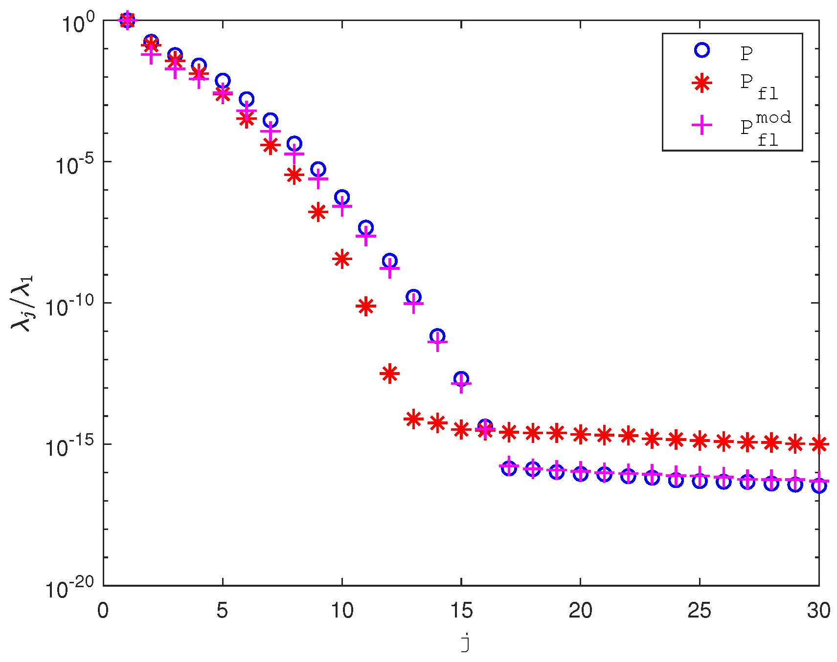
First, we examine the normalized eigenvalues (ratios to the largest eigenvalues) of the controllability Gramian P, the frequency-limited controllability Gramian P f l , and its modified version P f l mod , as shown in Figure 2. The Gramians P, P f l and P f l mod are accurately computed using MATLAB’s dlyap routine, while the matrix-valued function F ( δ ω ) B or B f l mod is handled using the integral routine. Eigenvalues smaller than 10 16 are discarded. As seen in the figure, the eigenvalues of P f l decay slightly faster than those of P and P f l mod , with their decay patterns being nearly identical. These results are consistent with the theoretical analysis presented in [22], suggesting that the frequency-limited Gramians P f l and Q f l can be effectively approximated using low-rank factors.
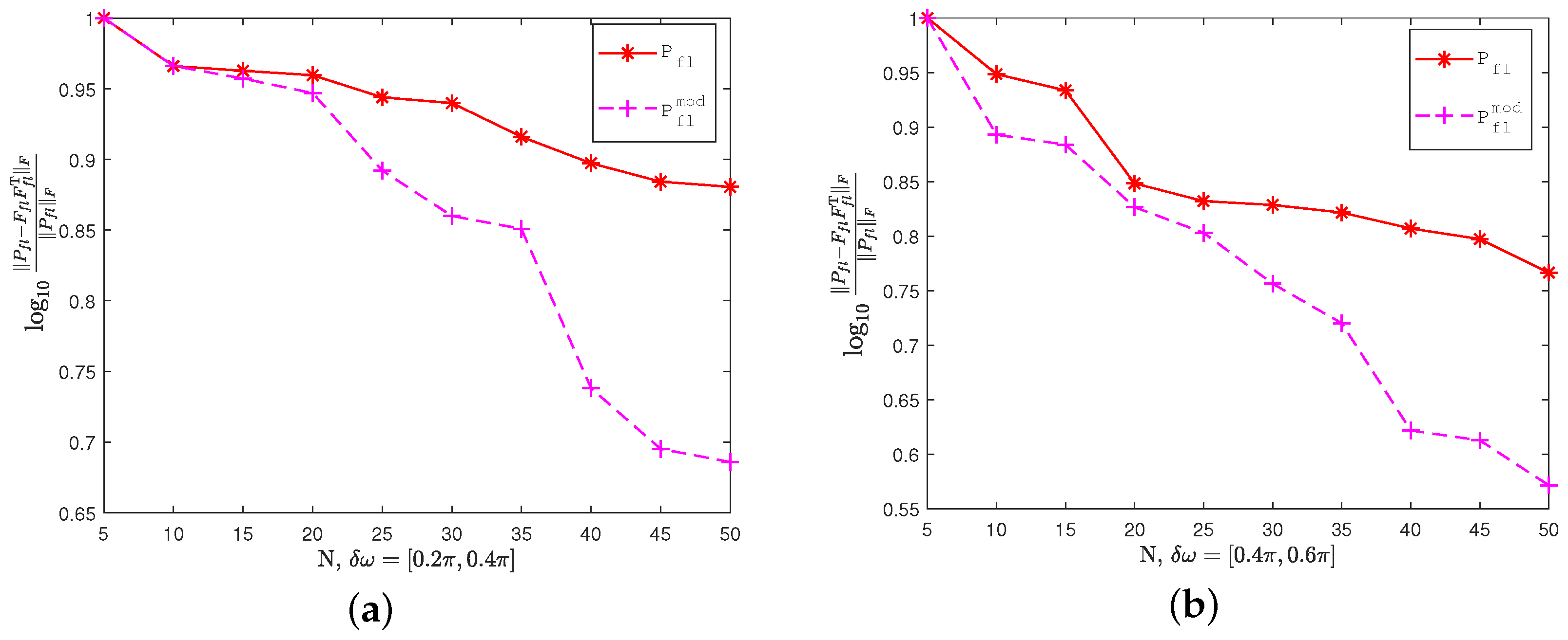
Next, to evaluate the performance of low-rank approximation for P f l and P f l mod using Laguerre functions, we plot the relative errors in a logarithmic scale
log 10 P f l F f l F f l T F P f l F and log 10 P f l mod F f l mod F f l mod T F P f l mod F
with respect to the truncation term N in the frequency intervals [ 0.2 π , 0.4 π ] and [ 0.4 π , 0.6 π ] , as shown in Figure 3. The results indicate an exponential decay in errors as the truncation term N increases. According to [20], the orthogonal polynomials expansion of a Lebesgue-measurable function converges uniformly, leading to optimal least-squares error approximation. Therefore, even a modest order of approximation can yield high accuracy.
We also implemented Moore’s BT and frequency-limited BT using the low-rank factors of the respective Gramians. For Moore’s BT, the low-rank factors of the Gramians P and Q were computed using the dlyapchol routine in MATLAB. Algorithms 1 and 2 based on Laguerre functions were used to calculate the low-rank factors of the frequency-limited Gramians P f l and Q f l along with their modifications P f l mod and Q f l mod . The parameters are listed in Table 1 with the Laguerre parameter α = ω 2 + ω 1 2 , where 0 ω 1 < ω 2 π . Given a tolerance t o l = 10 8 , the order r of the ROM is adaptively determined by the indicator δ t o l .
To assess the approximation quality of the constructed ROMs, we used the following relative error:
E ( ω ) = | G ( e j ω ) G r ( e j ω ) | / | G ( e j ω ) | , ω [ 0 , π ]
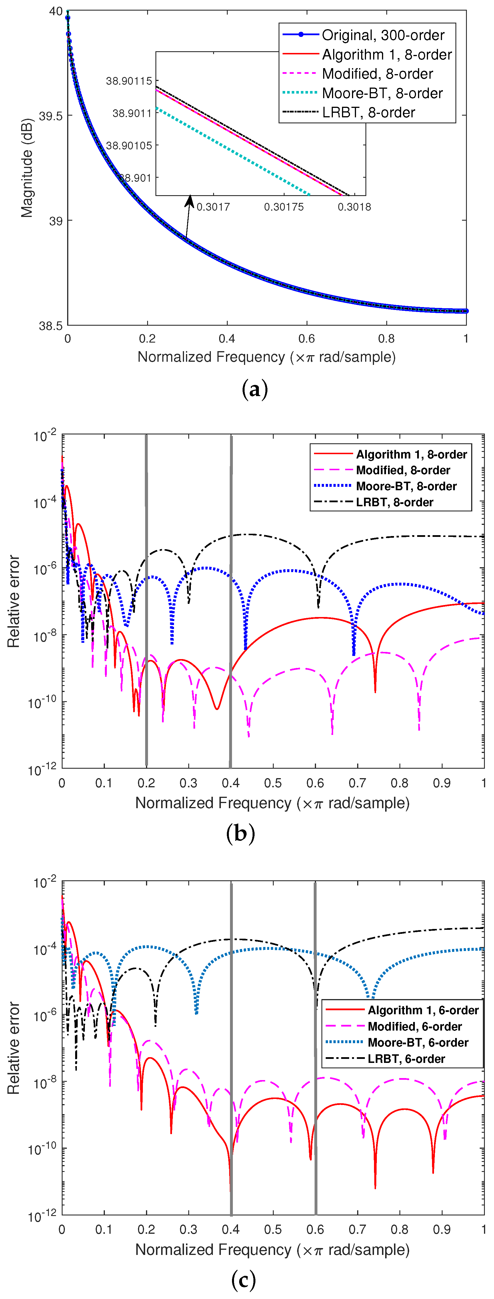
where G ( z ) and G r ( z ) represent the transfer function matrices of the original system and the ROMs, respectively. The magnitude plots of G ( z ) , G r ( z ) and the relative errors E ( ω ) obtained using the MATLAB freqz routine are shown in Figure 4, with the frequency interval boundaries ω 1 and ω 2 indicated by thick vertical lines.
Next, we compared the performance of our proposed low-rank MOR algorithms with traditional methods. Specifically, we evaluated Moore’s BT, FLBT, and the proposed Laguerre-based algorithms in terms of computational time and approximation error.
From Table 2, it is evident that the proposed Laguerre-based algorithms exhibit superior approximation accuracy compared to traditional methods such as Moore’s BT and FLBT. Furthermore, the computational time is significantly reduced, especially when compared to methods that require the direct solution of Lyapunov equations. The proposed approach also uses less memory, making it more suitable for large-scale systems.
The simulation results show that all four ROMs demonstrate superior performance in approximating the frequency responses of the original system. In the considered frequency intervals, it is evident that the approximation achieved by Algorithm 1 and Algorithm 1 surpasses that of Moore’s BT and LRBT with the same reduced order r. Compared to other frequency-limited BT methods, our proposed approach involves computing an N-dimensional integral matrix of Laguerre functions and its subsequent decomposition. This method offers the advantage of generating ROMs with high accuracy, particularly for small and medium-sized systems, while avoiding the complexity of matrix-valued functions and the direct solution of related generalized Lyapunov equations. This makes it particularly suitable for frequency-limited MOR of larger-scale systems.

5. Conclusions

This paper presents a novel approach to frequency-limited MOR for linear discrete-time systems leveraging low-rank approximations of Gramians. We introduce two MOR algorithms based on Laguerre functions, which differ from traditional methods that rely on solving generalized Lyapunov equations. These algorithms utilize Laguerre expansion coefficient vectors computed using recursive formulas to derive low-rank factors of frequency-limited controllability and observability Gramians, thereby ensuring computational efficiency. Additionally, a Laguerre-based frequency-limited low-rank MOR algorithm is proposed in combination with the modified frequency-limited BT method.
The proposed algorithms are demonstrated to be effective and efficient through numerical examples. However, to further enhance the approach’s performance, careful selection of the Laguerre parameter α is essential. Although there are established methods for parameter selection in frequency-free or infinite-frequency MOR in linear systems [24,25], the optimal choice of parameters for frequency-limited or more general cases remains an open question. Future research should focus on addressing this challenge in order to refine the proposed method and extend its applicability to more complex scenarios such as nonlinear and bilinear systems, which could ultimately provide more robust solutions for large-scale systems analysis and simulations.

Author Contributions

Methodology, Z.S. and Q.-Y.S.; Software, Z.S.; Writing—original draft, Z.S.; Writing—review & editing, Q.-Y.S. and U.Z.; Supervision, Q.-Y.S. and U.Z.; Funding acquisition, U.Z. All authors have read and agreed to the published version of the manuscript.

Funding

This work was supported by the National Natural Science Foundation of China (NSFC) under grants 62273059 and 62350410484 and in part by the High-End Foreign Expert Programs No. G2023027005L granted by the State Administration of Foreign Experts Affairs (SAFEA).

Data Availability Statement

The original contributions presented in the study are included in the article; further inquiries can be directed to the corresponding author.

Conflicts of Interest

The authors declare no conflicts of interest.

References

  1. Antoulas, A.C. Approximation of Large-Scale Dynamical Systems; SIAM: Philadelphia, PA, USA, 2005. [Google Scholar]
  2. Jiang, Y.L. Model Order Reduction Methods; Science Press: Beijing, China, 2010. [Google Scholar]
  3. Moore, B. Principal component analysis in linear systems: Controllability, observability, and model reduction. IEEE Trans. Autom. Control 1981, 26, 17–32. [Google Scholar] [CrossRef]
  4. Gugercin, S.; Antoulas, A.C. A survey of model reduction by balanced truncation and some new results. Int. J. Control 2004, 77, 748–766. [Google Scholar] [CrossRef]
  5. Zulfiqar, U.; Du, X.; Song, Q.Y.; Sreeram, V. On frequency-and time-limited μH2-optimal model order reduction. Automatica 2023, 153, 111012. [Google Scholar] [CrossRef]
  6. Song, Q.Y.; Zulfiqar, U.; Du, X. Finite-frequency model order reduction of linear and bilinear systems via low-rank approximation. J. Comput. Appl. Math. 2025, 457, 116287. [Google Scholar] [CrossRef]
  7. Gawronski, W.; Juang, J.N. Model reduction in limited time and frequency intervals. Int. J. Syst. Sci. 1990, 21, 349–376. [Google Scholar] [CrossRef]
  8. Wang, D.; Zilouchian, A. Model reduction of discrete linear systems via frequency-domain balanced structure. IEEE Trans. Circuits Syst. Fundam. Theory Appl. 2000, 47, 830–837. [Google Scholar] [CrossRef]
  9. Ghafoor, A.; Sreeram, V. Model reduction via limited frequency interval Gramians. IEEE Trans. Circuits Syst. I Regul. Pap. 2008, 55, 2806–2812. [Google Scholar] [CrossRef]
  10. Imran, M.; Ghafoor, A. Stability preserving model reduction technique and error bounds using frequency-limited Gramians for discrete-time systems. IEEE Trans. Circuits Syst. II Express Briefs 2014, 61, 716–720. [Google Scholar] [CrossRef]
  11. Kumar, D.; Sreeram, V.; Du, X. Model reduction using parameterized limited frequency interval Gramians for 1-D and 2-D separable denominator discrete-time systems. IEEE Trans. Circuits Syst. I Regul. Pap. 2018, 65, 2571–2580. [Google Scholar] [CrossRef]
  12. Toor, H.I.; Imran, M.; Ghafoor, A.; Kumar, D.; Sreeram, V.; Rauf, A. Frequency limited model reduction techniques for discrete-time systems. IEEE Trans. Circuits Syst. II Express Briefs 2019, 67, 345–349. [Google Scholar] [CrossRef]
  13. Batool, S.; Imran, M. Stability preserving model reduction technique for weighted and limited interval discrete-time systems with error bound. IEEE Trans. Circuits Syst. II Express Briefs 2021, 68, 3281–3285. [Google Scholar] [CrossRef]
  14. Xiao, Z.H.; Fang, Y.X.; Jiang, Y.L. Laguerre-Based Low-Rank Balanced Truncation of Discrete-Time Systems. IEEE Trans. Circuits Syst. II Express Briefs 2023, 70, 3014–3018. [Google Scholar] [CrossRef]
  15. Fang, Y.X.; Xiao, Z.H.; Qi, Z.Z. Low-rank balanced truncation of discrete time-delay systems based on Laguerre expansions. J. Frankl. Inst. 2024, 361, 106752. [Google Scholar] [CrossRef]
  16. Xiao, Z.H.; Jiang, Y.L.; Qi, Z.Z. Dimension reduction based on time-limited cross Gramians for bilinear systems. J. Comput. Appl. Math. 2025, 457, 116302. [Google Scholar] [CrossRef]
  17. Pernebo, L.; Silverman, L. Model reduction via balanced state space representations. IEEE Trans. Autom. Control 1982, 27, 382–387. [Google Scholar] [CrossRef]
  18. Al-Saggaf, U.; Franklin, G. An error bound for a discrete reduced order model of a linear multivariable system. IEEE Trans. Autom. Control 1987, 32, 815–819. [Google Scholar] [CrossRef]
  19. Horta, L.G.; Juang, J.N.; Longman, R.W. Discrete-time model reduction in limited frequency ranges. J. Guid. Control Dyn. 1993, 16, 1125–1130. [Google Scholar] [CrossRef]
  20. Szegö, G. Orthogonal Polynomials; American Mathematical Society: New York, NY, USA, 1939. [Google Scholar]
  21. Samuel, E.R.; Knockaert, L.; Dhaene, T. Model order reduction of time-delay systems using a Laguerre expansion technique. IEEE Trans. Circuits Syst. I Regul. Pap. 2014, 61, 1815–1823. [Google Scholar] [CrossRef]
  22. Benner, P.; Kurschner, P.; Saak, J. Frequency-limited balanced truncation with low-rank approximations. SIAM J. Sci. Comput. 2016, 38, A471–A499. [Google Scholar] [CrossRef]
  23. Imran, M.; Ghafoor, A. Frequency limited model reduction techniques with error bounds. IEEE Trans. Circuits Syst. II Express Briefs 2017, 65, 86–90. [Google Scholar] [CrossRef]
  24. Knockaert, L.; De Zutter, D. Stable Laguerre-SVD reduced-order modeling. IEEE Trans. Circuits Syst. I Fundam. Theory Appl. 2003, 50, 576–579. [Google Scholar] [CrossRef]
  25. Xiao, Z.H.; Song, Q.Y.; Jiang, Y.L.; Qi, Z.Z. Model order reduction of linear and bilinear systems via low-rank Gramian approximation. Appl. Math. Model. 2022, 106, 100–113. [Google Scholar] [CrossRef]
  26. Davis, T.A. Direct Methods for Sparse Linear Systems; SIAM: Philadelphia, PA, USA, 2006. [Google Scholar]
  27. Saad, Y. Iterative Methods for Sparse Linear Systems; SIAM: Philadelphia, PA, USA, 2003. [Google Scholar]
  28. Jiang, Y.L.; Wang, W.G. H2 optimal model order reduction of the discrete system on the product manifold. Appl. Math. Model. 2019, 69, 593–603. [Google Scholar] [CrossRef]
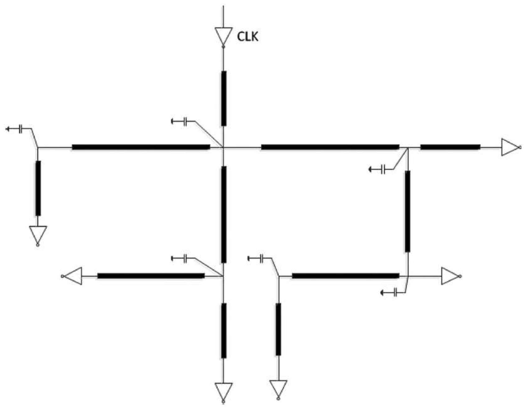
Figure 1. Interconnect layout in IC chips.
Mathematics 13 00448 g001
Figure 2. Normalized eigenvalues of the Gramians P, P f l , and P f l mod .
Mathematics 13 00448 g002
Figure 3. Relative errors in logarithmic sense of the Gramians P f l and P f l mod via Laguerre functions: (a) relative errors in [ 0.2 π , 0.4 π ] and (b) relative errors in [ 0.4 π , 0.6 π ] .
Mathematics 13 00448 g003
Figure 4. Results of the ROMs obtained by different BT versions: (a) magnitude plots of the original system and the ROMs, (b) relative errors E ( ω ) of the ROMs with the frequency interval δ ω = [ 0.2 π , 0.4 π ] , and (c) relative errors E ( ω ) of the ROMs with the frequency interval δ ω = [ 0.4 π , 0.6 π ] .
Mathematics 13 00448 g004
Table 1. Settings of the relevant parameters.
δ ω α N tol r
[ 0.2 π , 0.4 π ] 0.3 π 10 10 8 8
[ 0.4 π , 0.6 π ] 0.5 π 10 10 8 6
Table 2. The computational time and approximation error of the ROMs obtained by different methods.
MethodTime (Second)Relative ErrorRemark
δ ω = [0.2π, 0.4π] δ ω = [0.4π, 0.6π]
Algorithm 11.7542.025 × 10−82.051 × 10⁻⁹Low-rank (frequency-limited)
Modified1.7391.391 × 10−99.742 × 10⁻⁹Improved stability
Moore-BT14.7272.804 × 10−66.362 × 10⁻⁵Standard
LRBT0.8997.213 × 10−61.257 × 10⁻⁴Low-rank (infinite-frequency)
Disclaimer/Publisher’s Note: The statements, opinions and data contained in all publications are solely those of the individual author(s) and contributor(s) and not of MDPI and/or the editor(s). MDPI and/or the editor(s) disclaim responsibility for any injury to people or property resulting from any ideas, methods, instructions or products referred to in the content.