The Proximal Alternating Direction Method of Multipliers for a Class of Nonlinear Constrained Optimization Problems

Abstract

This paper presents a class of proximal alternating direction multiplier methods for solving nonconvex, nonsmooth optimization problems with nonlinear coupled constraints. The key feature of the proposed algorithm is that we use a linearized proximal technique to update the primary variables, followed by updating the dual variables using a discounting approach. This approach eliminates the requirement for an additional proxy function and then simplifies the optimization process. In addition, the algorithm maintains fixed parameter selection throughout the update process, removing the requirement to adjust parameters to ensure the decreasing nature of the generated sequence. Building on this framework, we establish a Lyapunov function with sufficient decrease and a lower bound, which is essential for analyzing the convergence properties of the algorithm. We rigorously prove both the subsequence convergence and the global convergence of the algorithm and ensure its robustness and effectiveness in solving complex optimization problems. Our paper provides a solid theoretical foundation for the practical application of this method in solving nonconvex optimization problems with nonlinear coupled constraints.

1. Introduction

This paper considers the following nonconvex, nonsmooth optimization problem with nonlinear coupled constraints:

$$minf\left(x\right)+g\left(x\right)+p\left(y\right),$$

$$\mathrm{s}.\mathrm{t}.h\left(x\right)+By=0.$$

(1)

where $x\in {\mathbb{R}}^n,y\in {\mathbb{R}}^m,f:{\mathbb{R}}^n\to \mathbb{R}\cup \{\infty \}$ is a proper lower semicontinuous function, $g:{\mathbb{R}}^n\to \mathbb{R}$ is a continuously differentiable function with local Lipschitz continuous gradients, $p:{\mathbb{R}}^m\to \mathbb{R}$ is a function with local Lipschitz continuous gradients $L_p$, where $L_p>0$, and $h:{\mathbb{R}}^n\to {\mathbb{R}}^q$ is a mapping with a locally continuous Jacobian matrix. $B\in {\mathbb{R}}^{q\times m}$ is a full-row rank matrix with the smallest eigenvalue $\lambda \left(B{B}^T\right)>0$.

Problem (1) is equivalent to many important problems, such as the risk parity portfolio selection problem [1], the robust phase recovery problem [2], and generative adversarial networks (GANs) [3]. When $B=-I$ (where I is the identity matrix), problem (1) is equivalent to the following problem:

$$minf\left(x\right)+g\left(x\right)+p\left(h\right(x\left)\right).$$

(2)

The typical example of problem (2) is the following Logistic Matrix Factorization problem [4]:

$$min\sum _{i=1}^m\sum _{j=1}^n\left((1+c{y}_{ij}-y_{ij})log\left(1+exp\left(u_i{v}_j^T\right)\right)-c{y}_{ij}{u}_i{v}_j^T\right)+{\displaystyle \frac{{\lambda }_d}{2}}{\parallel U\parallel }_F^2+{\displaystyle \frac{{\lambda }_t}{2}}{\parallel V\parallel }_F^2,$$

(3)

where elements $y_{ij}\in \{0,1\},{\lambda }_d,$ and ${\lambda }_t$ are regularization coefficients, and $c>0$ is a given constant.

In previous studies, when problem (1) is convex and involves linear coupled constraints, that is, $h\left(x\right)$ is an affine mapping, the alternating direction multiplier method (ADMM) has been extensively studied in many studies. In particular, when $h\left(x\right)=Ax$ and A and B are both full-rank, the global convergence of ADMM was established in references [5,6]. Researchers have found that many limitations arise when the problem is set as convex, while nonconvex formulations can better describe the problem model. So, the focus of research gradually shifted toward applying ADMM to nonconvex optimization problems. For example, references [7,8,9,10] established the global convergence of ADMM for nonconvex models with linear constraints.

Although the formulation of nonconvex problems has addressed some practical scenarios, the limitations of linear coupled constraint problems become evident as real-world constraints increase. As a result, researchers have shifted their focus to the study of nonlinear coupled constraint problems. For nonlinear coupled constraint problems, paper [11] proposed the concept of an information region within the Lagrange algorithm framework, where the boundedness of the multiplier sequence is a key assumption for the effect of the information region. The selection of parameters in the paper is related to the upper bound constant of the multiplier sequence, and in practice, determining the upper bound for the multipliers can be very challenging. Building on the idea of an information region from [11], paper [12] designed a proximal linearized alternating direction multiplier method with a backtracking process. Although convergence analysis does not rely on the boundedness of the multiplier sequence, it requires dynamically generated parameters during the backtracking process to ensure the boundedness of the generated sequence. Paper [13] used the upper bound minimization method to update the primal block variables. Building on this, paper [4] introduced inertia techniques and proposed a convergent alternating direction multiplier method with scaling factors to establish update rules. However, this requires the use of appropriate proxy functions to recover proximal points and proximal gradient descent steps, which is also challenging in practice.

In this paper, we propose a proximal linearized alternating direction multiplier method for problem (1). The core idea of this method is to use the proximal linearized alternating direction multiplier method and update the dual variables using a discount strategy. This method does not require selecting an additional proxy function and the parameter selection is fixed, eliminating the need to adjust the parameters to ensure the decreasing nature of the generated sequence, which leads to the convergence analysis of the algorithm.

The structure of this paper is as follows. Section 2 introduces the preliminary knowledge required for the convergence analysis of the algorithm. Section 3 describes the algorithm in detail and provides the convergence theorem. Section 4 presents the numerical experimental results of the algorithm for the non-negative matrix factorization problem. Section 5 concludes the paper and provides final remarks. In the Appendix A, we provide the proof process for some propositions.

2. Materials and Methods

In this section, we present the preliminaries needed for the convergence analysis. Based on the variational analysis of the problem (refer to [14]), we introduce the following constraint qualification conditions for problem (1). Here, $\nabla h(·)\in {\mathbb{R}}^{q\times n}$ represents the Jacobian matrix of h.

Definition 1

(Constraint Qualification [13]). A point $x\in {\mathbb{R}}^n$ satisfies the constraint qualification (CQ) for problem (1) if the following conditions hold:

(i) 

The subdifferential of f in x is regular.

(ii) 

${\partial }^{\infty }f\left(x\right)\cap \nabla h{\left(x\right)}^T=\left\{0\right\}$, i.e., the limiting subdifferential of f at x does not overlap with the range of the transpose of the gradient of the mapping hat x.

The [CQ] conditions ensure the smoothness and regularity of the constraint set, providing the necessary subdifferential calculus rules to establish the necessary first-order optimality conditions for problem (1).

Lemma 1

(First-Order Optimality Condition). Let $(x^{*},y^{*})\in {\mathbb{R}}^n\times {\mathbb{R}}^m$ be a local minimum of problem (1), and let $x^{*}$ satisfy the [CQ] condition. Then, we have the following:

(i) 

$h\left(x^{*}\right)+B{y}^{*}=0.$

(ii) 

There exists $u^{*}\in {\mathbb{R}}^q$ such that

$$0\in {\partial }_x(f\left(x^{*}\right)+g\left(x^{*}\right))+{\nabla }_{x}h{\left(x^{*}\right)}^T{u}^{*},{\nabla }_q\left(y^{*}\right)+B^T{u}^{*}=0,h\left(x^{*}\right)+B{y}^{*}=0.$$

This paper mainly considers the nonconvex and nonsmooth problem (1). Therefore, we provide some definitions and lemmas for convergence analysis [14,15,16].

Definition 2

(Subdifferential). Let E be a Euclidean vector space, and let $\Psi :E\to (-\infty ,\infty ]$ be a proper lower semicontinuous function. If $z\in dom(\Psi )$, then we have the following:

(i) 

The Fréchet (regular) subdifferential of Ψ at Z, denoted by $\partial \widehat{\Psi }\left(z\right)$, is defined as follows: For any vector $v\in E$, we have

$$\Psi \left(x\right)\ge \Psi \left(z\right)+\langle v,x-z\rangle +o(\parallel x-z\parallel ).$$

(ii) 

The limiting subdifferential of Ψ at Z, denoted by $\partial \Psi \left(z\right)$, is defined as follows: For any vector $v\in E$, there exists a sequence ${\left\{z^k\right\}}_{k\in \mathbb{N}}$ and ${\left\{v^k\right\}}_{k\in \mathbb{N}}$ such that $z^k\to z$, $\Psi \left(z^k\right)\to \Psi \left(z\right)$, $v^k\in \partial \widehat{\Psi }\left(z^k\right)$, and $v^k\to v$.

(iii) 

The horizontal subdifferential of Ψ at Z, denoted by ${\partial }^{\infty }\Psi \left(z\right)$, is similar to the definition in (ii), but for some real number sequence $t^k\to 0$, we do not have $v^k\to v$, but instead, $t^k{v}^k\to v$. For $z\notin dom(\Psi )$, we define $\partial \widehat{\Psi }\left(z\right)=\partial \Psi \left(z\right)={\partial }^{\infty }\Psi \left(z\right)=\varnothing$.

Proposition 1.

Let $\Psi :\mathbb{R}\to (-\infty ,\infty ]$ be an extended value function, and $\phi :{\mathbb{R}}^d\to \mathbb{R}$ be a smooth function. Then, we have the following:

$$\partial (\Psi +\phi )=\partial \Psi \left(x\right)+\nabla \phi \left(x\right),\forall x\in {\mathbb{R}}^d.$$

In problem (1), we consider the concept of Lipschitz functions and local Lipschitz continuity. Next, we provide the relevant concepts.

Definition 3.

Let $S\subseteq X$ be a non-empty set, and let $\phi :S\to Y$ be a continuous map on S. Then, we have the following:

(i) 

If $\parallel \phi \left(x\right)-\phi \left(z\right)\parallel \le L\parallel x-z\parallel$ for all $x,z\in S$ and $L\ge 0$, then φ is L-Lipschitz continuous on S.

(ii) 

If for each $z\in S$, there exist $ϵ\left(z\right)>0,L_{ϵ}\left(z\right)\ge 0$, and a neighborhood $N_{ϵ}\left(z\right):=\{x\in S:\parallel x-z\parallel <ϵ\left(z\right)\}$ such that φ is $L_{ϵ}\left(z\right)$-Lipschitz continuous on $N_{ϵ}\left(z\right)$, i.e.,

$$\parallel \phi \left(x\right)-\phi \left(z\right)\parallel \le L_{ϵ}\left(z\right)\parallel x-z\parallel ,\forall x,z\in N_{ϵ}\left(z\right).$$

When (i) or (ii) holds for $S\equiv X$, $\phi$ is called L-Lipschitz continuous or locally Lipschitz continuous, respectively.

Lemma 2

(Local Lipschitz Continuity of $\nabla \varphi$ [12]). The function $\varphi (x,y,u):=g\left(x\right)+\langle u,h\left(x\right)+By\rangle +{\displaystyle \frac{\rho }{2}}{\parallel h\left(x\right)+By\parallel }^2$ satisfies that for every non-empty and compact set $C\subset {\mathbb{R}}^n\times {\mathbb{R}}^m\times {\mathbb{R}}^q$, there exists $L_C\ge 0$ such that

$$\parallel \nabla \varphi \left(x\right)-\nabla \varphi \left(z\right)\parallel \le L_C\parallel x-z\parallel ,\forall x,z\in C.$$

This means that $\nabla \varphi$ is locally Lipschitz continuous.

Proposition 2

(Local Lipschitz Continuity and Compact Sets [17]). Let $S\subseteq X$ be a non-empty set, and let the mapping $\phi :X\to Y$ be locally Lipschitz continuous on S. Then, for every non-empty compact set $C\subseteq S$, there exists $L\ge 0$ such that φ is L-Lipschitz continuous on C, i.e.,

$$\parallel \phi \left(x\right)-\phi \left(z\right)\parallel \le L_C\parallel x-z\parallel ,\forall x,z\in C.$$

Proposition 3

(Differential Mapping and Lipschitz Continuity [18]). Let $\phi :X\to Y$ be a $C^1$-mapping. Then, the following statements hold:

(i) 

φ is locally Lipschitz continuous.

(ii) 

Let $B\subset X$ be a closed ball, i.e., $B=\{x:\parallel x-z\parallel \le r\}$ for some $z\in X$ and $r\in (0,\infty ]$. If φ is L-Lipschitz continuous on B, with $L_B\ge 0$, then $\parallel \nabla \phi \left(x\right)\parallel \le L_B$, for all $x\in B$.

3. Results

3.1. Algorithm

First, we define the augmented Lagrangian function associated with problem (1), $L:{\mathbb{R}}^n\times {\mathbb{R}}^m\times {\mathbb{R}}^q\to (-\infty ,\infty ]$, with penalty parameter $\rho >0$:

$$L_{\rho }(x,y,u):=f\left(x\right)+g\left(x\right)+p\left(y\right)+\langle u,h\left(x\right)+By\rangle +{\displaystyle \frac{\rho }{2}}{\parallel h\left(x\right)+By\parallel }^2,$$

(4)

where $\parallel ·\parallel$ denotes the standard Euclidean $l_2$-norm.

To distinguish between the smooth and nonsmooth components in L, we define $\varphi :{\mathbb{R}}^n\times {\mathbb{R}}^m\times {\mathbb{R}}^q\to \mathbb{R}$ as

$$\varphi (x,y,u):=g\left(x\right)+\langle u,h\left(x\right)+By\rangle +{\displaystyle \frac{\rho }{2}}{\parallel h\left(x\right)+By\parallel }^2.$$

(5)

Thus, $L_{\rho }(x,y,u)=f\left(x\right)+p\left(y\right)+\varphi (x,y,u).$

Next, we present Algorithm 1 proposed in this paper.

Algorithm 1 Proximal Linearized ADMM (PADMM)

Input: Initial values $(x^0,y^0,u^0)\in {\mathbb{R}}^n\times {\mathbb{R}}^m\times {\mathbb{R}}^q$, $\theta >0$, $\eta >0$, $\tau \in [0,1)$, and let $k\to 0$.

Repeat:

Primal update:

$$x^{k+1}\in arg\underset{x\in {\mathbb{R}}^n}{min}\left\{{\phi }_k\left(x\right):=f\left(x\right)+\langle {\nabla }_x\varphi (x^k,y^k,u^k),x\rangle +{\displaystyle \frac{\eta }{2}}{\parallel x-x^k\parallel }^2\right\}$$ (6)

$$y^{k+1}\in arg\underset{y\in {\mathbb{R}}^m}{min}\left\{{\psi }_k\left(y\right):=\varphi (x^{k+1},y,u^k)+\langle \nabla p\left(y^k\right),y\rangle +{\displaystyle \frac{\theta }{2}}{\parallel y-y^k\parallel }^2\right\}$$ (7)

Dual update:

$$u^{k+1}=(1-\tau )u^k+\rho \left(h\left(x^{k+1}\right)+B{y}^{k+1}\right)$$ (8)

Until the convergence criterion is satisfied.

Remark 1.

For Equation (6), we first provide the properties of the proximal mapping [14]: when $\xi :{\mathbb{R}}^d\to (-\infty ,\infty ]$ be a proper lower semicontinuous function, with ${inf}_{{\mathbb{R}}^d}\xi >-\infty$, let $x\in {\mathbb{R}}^d$. When $t>0$, the proximal mapping ${\mathit{prox}}_{\xi /t}\left(x\right)$ is defined as

$${prox}_{\xi /t}\left(x\right)=argmin\left\{\xi \left(z\right)+{\displaystyle \frac{t}{2}}{\parallel z-x\parallel }^2:z\in {\mathbb{R}}^d\right\}.$$

So, Equation (6) is essentially a proximal gradient update step:

$$\begin{array}{cc}\hfill x^{k+1}& \in argmi{n}_{x\in {\mathbb{R}}^n}\left\{f\left(x\right)+\langle {\nabla }_x\varphi (x^k,y^k,u^k),x\rangle +{\displaystyle \frac{\eta }{2}}{\parallel x-x^k\parallel }^2\right\}\hfill \\ \hfill & ={\mathit{prox}}_{{\eta }^{-1}f}\left(x^k-{\eta }^{-1}{\nabla }_x\varphi (x^k,y^k,u^k)\right).\hfill \end{array}$$

(9)

For Equation (7), we note that ψ is a strongly convex function. Since for any $\theta >0$ matrix $\rho B^{\top }B+\theta I>0$, we can derive the explicit update expression for $y^{k+1}$ from the first-order optimality condition of (7):

$$\begin{array}{c}\hfill y^{k+1}={(\rho B^{\top }B+\theta I)}^{-1}\left(\theta y^k-B^{\top }(u^k+\rho h\left(x^{k+1}\right))-\nabla q\left(y^k\right)\right).\end{array}$$

(10)

For Equation (8), we adopt a discount update scheme:

$$\begin{array}{cc}\hfill u^{k+1}& =(1-\tau )u^k+\rho (h\left(x^{k+1}\right)+B{y}^{k+1})\hfill \\ \hfill & ={(1-\tau )}^2{u}^{k-1}+(1-\tau )\rho (h\left(x^k\right)+B{y}^k)+\rho (h\left(x^{k+1}\right)+B{y}^{k+1})\hfill \\ \hfill & ⋮\hfill \\ \hfill & ={(1-\tau )}^{k+1}{u}^0+\sum _{l=0}^k{(1-\tau )}^{k-l}\rho \left(h\left(x^{l+1}\right)+B{y}^{l+1}\right).\hfill \end{array}$$

(11)

In contrast, the dual update for the ADMM method with nonlinear coupling constraints is typically

$$\begin{array}{cc}\hfill u^{k+1}& =u^k+\rho \left(h\left(x^{k+1}\right)+B{y}^{k+1}\right)\hfill \\ \hfill & =u^{k-1}+\rho \left(h\left(x^k\right)+B{y}^k\right)+\rho \left(h\left(x^{k+1}\right)+B{y}^{k+1}\right)\hfill \\ \hfill & ⋮\hfill \\ \hfill & =u^0+\sum _{l=0}^k\rho \left(h\left(x^{l+1}\right)+B{y}^{l+1}\right).\hfill \end{array}$$

(12)

In the proximal alternating direction method of multipliers (proximal ADMM), the primal and dual updates alternate until the stopping criteria are met.

3.2. Convergence Analysis

Our analysis will focus on the function $\varphi$. For the convenience of subsequent proofs, we first present some formulas:

$${\nabla }_x\varphi (x,y,u)=\nabla g\left(x\right)+\nabla h^T\left(x\right)(u+\rho (h\left(x\right)+By)),$$

(13)

$${\nabla }_y\varphi (x,y,u)=B^T(u+\rho (h\left(x\right)+By)),$$

(14)

$${\nabla }_u\varphi (x,y,u)=h\left(x\right)+By.$$

(15)

We also state the assumptions required for our proof. We assume that the functions g and p have lower bounds, that is, $g\left(x\right)>-\infty ,\forall x\in {\mathbb{R}}^n$ and $p\left(y\right)>-\infty ,\forall y\in {\mathbb{R}}^m.$

First, we provide the relationship between y and u.

Proposition 4.

Assume ${\widehat{u}}^k:=u^k+\rho (h\left(x^{k+1}\right)+B{y}^{k+1})$, for all $k\ge 1$; then, we have

$$\parallel u^{k+1}-u^k{\parallel }^2\le {\displaystyle \frac{1}{\lambda }}{\left(\theta \parallel y^{k+1}-y^k\parallel +(L_q+\theta )\parallel y^k-y^{k-1}\parallel \right)}^2.$$

(16)

Proof of Proposition 4.

We defer the proof to Appendix A.1.    □

Let $L_{\rho }^{+}(x^{k+1},y^{k+1},u^{k+1})=L_{\rho }(x^{k+1},y^{k+1},u^{k+1})-{\displaystyle \frac{\tau }{2\rho }}{\parallel u^{k+1}\parallel }^2$. For all $k\ge 1$, let this be the regularized AL function. We have the following proposition to quantify the change in the regularized AL function over successive iterations.

Proposition 5.

For all $k\ge 1$, we have

$$\begin{array}{cc}\hfill & L_{\rho }^{+}(x^{k+1},y^{k+1},u^{k+1})-L_{\rho }^{+}(x^k,y^k,u^k)\hfill \\ \hfill & \le -{\displaystyle \frac{\eta -L_C}{2}}\parallel x^{k+1}-x^k{\parallel }^2-\left({\displaystyle \frac{2\theta -L_q}{2}}-{\displaystyle \frac{(2-\tau ){\theta }^2}{\rho {\lambda }_{min}\left(B{B}^T\right)}}\right){\parallel y^{k+1}-y^k\parallel }^2\hfill \\ \hfill & +{\displaystyle \frac{(2-\tau ){(\theta +L_h)}^2}{\rho {\lambda }_{min}\left(B{B}^T\right)}}{\parallel y^k-y^{k-1}\parallel }^2.\hfill \end{array}$$

Proof of Proposition 5.

We defer the proof to Appendix A.2.    □

In particular, the authors of [19] built a general framework to establish convergence for nonconvex settings, comprising two key steps: (1) identifying a so-called sufficiently decreasing Lyapunov function and (2) establishing the lower boundness property of the Lyapunov function. The augmented Lagrangian (AL) function has often been used as the Lyapunov function in nonconvex settings. In Proposition 5, $L_{\rho }^{+}(x,y,u)$ is the regularized AL function. We observe that the sufficient descent property of the AL function can only hold when the primal update restricts the dual update, i.e., $\parallel u^{k+1}-u^k{\parallel }^2$, for the sufficient descent property of the AL function to hold. First, based on the ascent–descent relationship established in Proposition 6, we introduce the Lyapunov function ${\Gamma }_{\beta }:{\mathbb{R}}^n\times {\mathbb{R}}^m\times {\mathbb{R}}^q\times {\mathbb{R}}^m\to (-\infty ,\infty ]$, defined as ${\Gamma }_{\beta }=L_{\rho }^{+}(x,y,u)+{\displaystyle \frac{\beta }{2}}{\parallel y-w\parallel }^2,$ where $\beta >0$ is a constant parameter required to ensure the sufficient descent and lower bound properties of the Lyapunov function. Next, we establish the sufficient descent property of the Lyapunov function. For convenience, we define the sequence ${\{z^k\equiv (x^k,y^k,u^k,y^{k-1})\}}_{k\ge 1}$ as a descent sequence for the Lyapunov function ${\Gamma }_{\beta }$. Based on Proposition 4 and Proposition 5, the following proposition can be easily obtained.

Proposition 6.

For $k\ge 1$,

$${\Gamma }_{\beta }\left(z^{k+1}\right)-{\Gamma }_{\beta }\left(z^k\right)\le -{\displaystyle \frac{\eta -L_C}{2}}\parallel x^{k+1}-x^k{\parallel }^2-{\alpha }_1\parallel y^{k+1}-y^k{\parallel }^2-{\alpha }_2{\parallel y^k-y^{k-1}\parallel }^2,$$

where $\lambda ={\lambda }_{min}\left(B{B}^T\right),{\alpha }_1={\displaystyle \frac{2\theta -L_p-\beta }{2}}-{\displaystyle \frac{(2-\tau ){\theta }^2}{\rho \lambda }}$, and ${\alpha }_2={\displaystyle \frac{\beta }{2}}-{\displaystyle \frac{(2-\tau ){(\theta +L_h)}^2}{\rho \lambda }}$.

This implies that when ${\displaystyle \frac{\eta -L_C}{2}}>0,{\alpha }_1>0$, and ${\alpha }_2>0$, the Lyapunov function we constructed maintains sufficient descent properties. Another key step for the convergence of the algorithm is to establish the lower bound properties of the Lyapunov function. To do so, we first prove the lower bound property of the Lagrange multipliers generated by the discounted dual update scheme.

Proposition 7.

Let ${\Delta }^k:=\parallel h\left(x^k\right)+B{y}^k\parallel$ be the constraint residual at iteration k, and let ${\Delta }^{max}=max\parallel h\left(x^k\right)+B{y}^k\parallel$ represent the maximum constraint residual over the feasible set. Algorithm 1, starting from any given initial dual variable $u^0$, guarantees that $\parallel u^k\parallel$ is bounded, i.e.,

$$\parallel u^k\parallel \le \parallel u^0\parallel +{\tau }^{-1}\rho {\Delta }^{max},$$

or equivalently,

$$\parallel u^k{\parallel }^2\le 2{\parallel u^0\parallel }^2+2{\tau }^{-2}{\rho }^2{\left({\Delta }^{max}\right)}^2.$$

Proof. 

From Equation (12), we have

$$\begin{array}{cc}\hfill \parallel u^k\parallel & {=\parallel (1-\tau )}^{k+1}{u}^0+\sum _{l=0}^k\rho {(1-\tau )}^{k-l}{\Delta }^{l+1}\parallel \hfill \\ \hfill & {\le \parallel (1-\tau )}^{k+1}{u}^0\parallel +\sum _{l=0}^k\parallel \rho {(1-\tau )}^{k-l}{\Delta }^{l+1}\parallel \hfill \\ \hfill & {\le \parallel (1-\tau )}^{k+1}{u}^0\parallel +\rho {\Delta }^{\max }{\displaystyle \frac{1-{(1-\tau )}^k}{\tau }}\hfill \\ \hfill & \le \parallel u^0\parallel +{\tau }^{-1}\rho {\Delta }^{\max }.\hfill \end{array}$$

   □

The first inequality follows from the triangle inequality, the second inequality comes from ${\Delta }^k\le {\Delta }^{\max }$, and the final inequality holds because $\tau \in (0,1)$. Furthermore, by applying the inequality ${\parallel a+b\parallel }^2\le {2\parallel a\parallel }^2+2{\parallel b\parallel }^2$, we can establish the lower bound property of the Lyapunov function.

Proposition 8.

For the sequence ${\left\{z^k\right\}}_{k\in K}$ generated by the algorithm, we have ${\Gamma }_{\beta }\left(z^k\right)>-\infty$ for all $k\in K$.

Proof. 

Observe the construction of ${\Gamma }_{\beta }\left(z^k\right)=L_{\rho }(x^k,y^k,u^k)-{\displaystyle \frac{\tau }{2\rho }}\parallel u^k{\parallel }^2+{\displaystyle \frac{\beta }{2}}{\parallel y^{k-1}-y^{k-2}\parallel }^2$. Clearly, ${\displaystyle \frac{\beta }{2}}{\parallel y^k-y^{k-1}\parallel }^2$ is non-negative and has a lower bound, and, by Proposition 7, since $\parallel u^k{\parallel }^2$ is bounded, $-{\displaystyle \frac{\tau }{2\rho }}{\parallel u^k\parallel }^2$ is also bounded. Therefore, we need to prove the boundedness of $L_{\rho }(x^k,y^k,u^k)$. Observe that $L_{\rho }(x^k,y^k,u^k)$, based on our assumptions, has $g>-\infty$ and $p>-\infty ,f>-\infty$, and ${\displaystyle \frac{\rho }{2}}{\parallel h\left(x\right)+By\parallel }^2$ is non-negative and has a lower bound. Thus, we only need to prove the lower bound of $\langle u,h\left(x\right)+By\rangle$. Based on dual update (10), we have

$$\begin{array}{cc}\hfill & \langle u^{k+1},h\left(x^{k+1}\right)+B{y}^{k+1}\rangle =\langle u^{k+1},{\displaystyle \frac{u^{k+1}-(1-\tau )u^k}{\rho }}\rangle \hfill \\ \hfill & =\langle u^{k+1},{\displaystyle \frac{1-\tau }{\rho }}(u^{k+1}-u^k)+{\displaystyle \frac{\tau }{\rho }}{u}^{k+1}\rangle \hfill \\ \hfill & ={\displaystyle \frac{\tau }{\rho }}{\parallel u^{k+1}\parallel }^2+{\displaystyle \frac{1-\tau }{\rho }}\langle u^{k+1},u^{k+1}-u^k\rangle \hfill \\ \hfill & ={\displaystyle \frac{\tau }{\rho }}{\parallel u^{k+1}\parallel }^2+{\displaystyle \frac{1-\tau }{2\rho }}\left(\parallel u^{k+1}-u^k{\parallel }^2+\parallel u^{k+1}{\parallel }^2-{\parallel u^k\parallel }^2\right)\hfill \end{array}$$

(17)

We know that $\parallel u^k{\parallel }^2$ is bounded, so we conclude that $L_{\rho }(x^k,y^k,u^k)$ has a lower bound. The proof is complete.    □

3.3. Main Result

To demonstrate the convergence result of the algorithm, we first define the notion of an approximate stationary solution.

Definition 4.

For all ϵ, when $(x^{*},y^{*},u^{*})$ is an ϵ-approximate stationary solution of problem (1), we have

$$\begin{array}{cc}\hfill & dist\left(\nabla f\left(x^{*}\right)+\nabla g\left(x^{*}\right)+\nabla h^T\left(x^{*}\right){\widehat{u}}^{*}+N\left(x^{*}\right),0\right)+dist\left({\nabla }_{y}p\left(y^{*}\right)+B^T{\widehat{u}}^{*},0\right)\hfill \\ \hfill & +\parallel h\left(x^{*}\right)+B{y}^{*}\parallel \le ϵ.\hfill \end{array}$$

Theorem 1.

Assume that the parameters used in the algorithm satisfy the conditions under which the lemmas hold. Then, we have the following:

(i) 

The sequences $\left\{x^k\right\}$, $\left\{y^k\right\}$, and $\left\{u^k\right\}$ generated by the algorithm are bounded and converge, i.e.,

$$x^{k+1}-x^k\to 0,y^{k+1}-y^k\to 0,u^{k+1}-u^k\to 0.$$

(ii) 

Suppose there is a limit point $(x^{*},y^{*},u^{*})$. Then, when ${\widehat{u}}^{*}=(1+\tau )u^{*}$, the point $(x^{*},y^{*},{\widehat{u}}^{*})$ is a $\tau {\rho }^{-1}\parallel u^{*}\parallel$-approximate stationary solution to problem (1).

Proof. 

From Proposition 6, we have

$$\sum _{k=1}^K\left({\Gamma }_{\beta }\left(z^k\right)-{\Gamma }_{\beta }\left(z^{k+1}\right)\right)\ge {\displaystyle \frac{\eta -L_C}{2}}\sum _{k=1}^K\parallel x^{k+1}-x^k{\parallel }^2+{\alpha }_1\sum _{k=1}^K\parallel y^{k+1}-y^k{\parallel }^2+{\alpha }_2\sum _{k=1}^K{\parallel y^k-y^{k-1}\parallel }^2.$$

Let $K\to \infty$, and we obtain

$${\Gamma }_{\beta }\left(z^1\right)-\underset{K\to \infty }{lim}{\Gamma }_{\beta }\left(z^{k+1}\right)\ge {\displaystyle \frac{\eta -L_C}{2}}\sum _{k=1}^{\infty }\parallel x^{k+1}-x^k{\parallel }^2+{\alpha }_1\sum _{k=1}^{\infty }\parallel y^{k+1}-y^k{\parallel }^2+{\alpha }_2\sum _{k=1}^{\infty }{\parallel y^k-y^{k-1}\parallel }^2.$$

Since ${\Gamma }_{\beta }\left(z^{k+1}\right)>-\infty$, we have

$$\infty >{\displaystyle \frac{\eta -L_C}{2}}\sum _{k=1}^{\infty }\parallel x^{k+1}-x^k{\parallel }^2+{\alpha }_1\sum _{k=1}^{\infty }\parallel y^{k+1}-y^k{\parallel }^2+{\alpha }_2\sum _{k=1}^{\infty }{\parallel y^k-y^{k-1}\parallel }^2.$$

This implies that

$$\parallel x^{k+1}-x^k\parallel \to 0,\parallel y^{k+1}-y^k\parallel \to 0,\parallel u^{k+1}-u^k\parallel \to 0.$$

Therefore, sequences $\left\{x^k\right\}$, $\left\{y^k\right\}$, and $\left\{u^k\right\}$ converge to $x^{*},y^{*}$, and $u^{*}$, i.e., as $K\to \infty$, we have $x^{k+1}\to x^{*},y^{k+1}\to y^{*}$, and $u^{k+1}\to u^{*},$ and also $x^{k+1}\to x^k,y^{k+1}\to y^k$, and $u^{k+1}\to u^k.$

From the dual updates, $(x^{*},y^{*},u^{*})$ satisfies

$$h\left(x^{*}\right)+B{y}^{*}=\tau {\rho }^{-1}{u}^{*}.$$

(18)

As we defined ${\widehat{u}}^k:=u^k+\rho (h\left(x^{k+1}\right)+B{y}^{k+1})$, we know that ${\widehat{u}}^k\to (1+\tau )u^{*}$. Thus, by setting ${\widehat{u}}^{*}=(1+\tau )u^{*}$, we have ${\widehat{u}}^k\to {\widehat{u}}^{*}$.

Next, for part (ii), we consider the first-order optimality conditions for the update when $k\ge 1$, and by taking $k\to \infty$, we have

$$0\in {\partial }_{x}f\left(x^{k+1}\right)+{\nabla }_x\varphi (x^k,y^k,u^k)+\eta (x^{k+1}-x^k)={\partial }_{x}f\left(x^{*}\right)+\nabla g\left(x^{*}\right)+\nabla h^T\left(x^{*}\right){\widehat{u}}^{*}.$$

(19)

$$0={\nabla }_{y}p\left(y^{*}\right)+B^T{\widehat{u}}^{*},h\left(x^{*}\right)+B{y}^{*}=\tau {\rho }^{-1}{u}^{*}.$$

(20)

From (19), according to [7], there exists $v^{k+1}\in N_x\left(x^{k+1}\right)$ such that

$$0={\nabla }_{x}f\left(x^{k+1}\right)+{\nabla }_x\varphi (x^k,y^k,u^k)+\eta (x^{k+1}-x^k)+v^{k+1}.$$

Thus, we obtain

$$0\in \nabla f\left(x^{*}\right)+\nabla g\left(x^{*}\right)+\nabla h^T\left(x^{*}\right){\widehat{u}}^{*}+N\left(x^{*}\right).$$

This leads to

$$dist\left(\nabla f\left(x^{*}\right)+\nabla g\left(x^{*}\right)+\nabla h^T\left(x^{*}\right){\widehat{u}}^{*}+N\left(x^{*}\right),0\right)=0,\mathrm{dist}\left({\nabla }_{y}p\left(y^{*}\right)+B^T{\widehat{u}}^{*},0\right)=0.$$

(21)

Therefore, from (18) and (21), we obtain

$$\begin{array}{cc}\hfill & dist\left(\nabla f\left(x^{*}\right)+\nabla g\left(x^{*}\right)+\nabla h^T\left(x^{*}\right){\widehat{u}}^{*}+N\left(x^{*}\right),0\right)+\mathrm{dist}\left({\nabla }_{y}p\left(y^{*}\right)+B^T{\widehat{u}}^{*},0\right)\hfill \\ & +\parallel h\left(x^{*}\right)+B{y}^{*}\parallel \le \tau {\rho }^{-1}\parallel u^{*}\parallel .\hfill \end{array}$$

Next, we consider the convergence of $u^{*}$ depending on $\tau$ and $\rho$, which we can still achieve by setting the initial points and parameters. First, from Proposition 7, we know that

$${\Gamma }_{\beta }\left(z^{k+1}\right)\le {\Gamma }_{\beta }\left(z^0\right),$$

and from (17), we obtain

$$\begin{array}{cc}\hfill Gamm{a}_{\beta }\left(z^{k+1}\right)& =f\left(x^{k+1}\right)+g\left(x^{k+1}\right)+p\left(y^{k+1}\right)+{\displaystyle \frac{\rho }{2}}\parallel h\left(x^{k+1}\right)+B{y}^{k+1}{\parallel }^2+{\displaystyle \frac{\tau }{2\rho }}{\parallel u^{k+1}\parallel }^2\hfill \\ \hfill & +{\displaystyle \frac{\beta }{2}}{\parallel y^k-y^{k-1}\parallel }^2+{\displaystyle \frac{1-\tau }{2\rho }}\left(\parallel u^{k+1}-u^k{\parallel }^2+\parallel u^{k+1}{\parallel }^2-{\parallel u^k\parallel }^2\right).\hfill \end{array}$$

Thus, we have

$${\displaystyle \frac{1-\tau }{2\rho }}\left(\parallel u^{k+1}{\parallel }^2-{\parallel u^k\parallel }^2\right)+{\displaystyle \frac{\tau }{2\rho }}{\parallel u^{k+1}\parallel }^2\le {\Gamma }_{\beta }\left(z^0\right).$$

(22)

This is because $f\left(x^{k+1}\right)\ge 0$, $g\left(x^{k+1}\right)\ge 0$, $p\left(y^{k+1}\right)\ge 0$, and the remaining terms are non-negative. Next, we prove by induction that ${\displaystyle \frac{\tau }{2\rho }}{\parallel u^{k+1}\parallel }^2\le {\Gamma }_{\beta }\left(z^0\right)$. For $k=0$, we can appropriately choose the initial point to satisfy the inequality. For k, assume ${\displaystyle \frac{\tau }{2\rho }}{\parallel u^k\parallel }^2\le {\Gamma }_{\beta }\left(z^0\right)$ and consider two cases for the $k+1$-th iteration: if $\parallel u^{k+1}{\parallel }^2\le {\parallel u^k\parallel }^2$, we can directly conclude that ${\displaystyle \frac{\tau }{2\rho }}\parallel u^{k+1}{\parallel }^2\le {\displaystyle \frac{\tau }{2\rho }}{\parallel u^k\parallel }^2\le {\Gamma }_{\beta }\left(z^0\right)$. If $\parallel u^{k+1}{\parallel }^2\ge {\parallel u^k\parallel }^2$, based on (22), we can again conclude the desired result. Therefore, we can infer that $\parallel u^{*}{\parallel }^2\le 2\rho {\tau }^{-1}{\Gamma }_{\beta }\left(z^0\right)$. Clearly, there exists a constant c such that ${\Gamma }_{\beta }\left(z^0\right)<c$. Thus, there exists an $ϵ$ such that ${\tau }^2{\rho }^{-2}{\parallel u^{*}\parallel }^2\le {ϵ}^2$. Therefore, we conclude the following:

$$\begin{array}{cc}\hfill & dist\left(\nabla f\left(x^{*}\right)+\nabla g\left(x^{*}\right)+\nabla h^T\left(x^{*}\right){\widehat{u}}^{*}+N\left(x^{*}\right),0\right)+\mathrm{dist}\left({\nabla }_{y}p\left(y^{*}\right)+B^T{\widehat{u}}^{*},0\right)\hfill \\ & +\parallel h\left(x^{*}\right)+B{y}^{*}\parallel \le \tau {\rho }^{-1}\parallel u^{*}\parallel .\hfill \end{array}$$

   □

4. Discussion

In this study, we tested the algorithm proposed in this paper on problem (3). All tests were conducted using Matlab R2023b on a Macbook Air M2.

We primarily focused on the application of the proposed algorithm to the Logistic Matrix Factorization problem. Problem (3) is written in the same form as problem (1):

$$\begin{array}{c}min g(U,V)+p\left(W\right)\\ s.t.UV-W=0.\end{array}$$

where $p\left(W\right)={\sum }_{i,j}\left((1+c{y}_{ij}-y_{ij})log(1+exp\left(W_{ij}\right))-c{y}_{ij}{W}_{ij}\right),$ and $g(U,V)={\displaystyle \frac{{\lambda }_d}{2}}{\parallel U\parallel }_F^2+{\displaystyle \frac{{\lambda }_t}{2}}{\parallel V\parallel }_F^2,f=0,h=UV.$ The augmented Lagrangian function for the problem is

$$L_{\rho }(U,V,W,u)=g(U,V)+q\left(W\right)+\langle u,UV-W\rangle +{\displaystyle \frac{\rho }{2}}{\parallel UV-W\parallel }^2.$$

From Equation (6), U is updated as follows:

$$\begin{array}{cc}\hfill U^{k+1}& \in argmin\left\{\langle \nabla g\left(U^k\right)+\nabla h{\left(U^k\right)}^T(u^k+\rho (U^k{V}^k-W^k)),U\rangle +{\displaystyle \frac{\eta }{2}}{\parallel U-U^k\parallel }^2\right\}\hfill \\ \hfill & ={\displaystyle \frac{1}{\eta }}\left(U^k-{\lambda }_d{U}^k+{\left(V^k\right)}^T(u^k+\rho (U^k{V}^k-W^k))\right).\hfill \end{array}$$

Similarly, for V,

$$\begin{array}{cc}\hfill V^{k+1}& \in argmin\left\{\langle \nabla g\left(V^k\right)+\nabla h{\left(V^k\right)}^T(u^k+\rho (U^k{V}^k-W^k)),V\rangle +{\displaystyle \frac{\eta }{2}}{\parallel V-V^k\parallel }^2\right\}\hfill \\ \hfill & ={\displaystyle \frac{1}{\eta }}\left(V^k-{\lambda }_t{V}^k+{\left(U^k\right)}^T(u^k+\rho (U^k{V}^k-W^k))\right).\hfill \end{array}$$

W is updated using the explicit expression in Equation (7):

$$W^{k+1}={(\rho +\theta )}^{-1}\left(\theta W^k-B^T(u^k+\rho \left(U^{k+1}{V}^{k+1}\right))-\nabla q\left(W^k\right)\right).$$

Finally, $u^{k+1}$ is updated as

$$u^{k+1}=(1-\tau )u^k+\rho (U^{k+1}{V}^{k+1}-W^{k+1}).$$

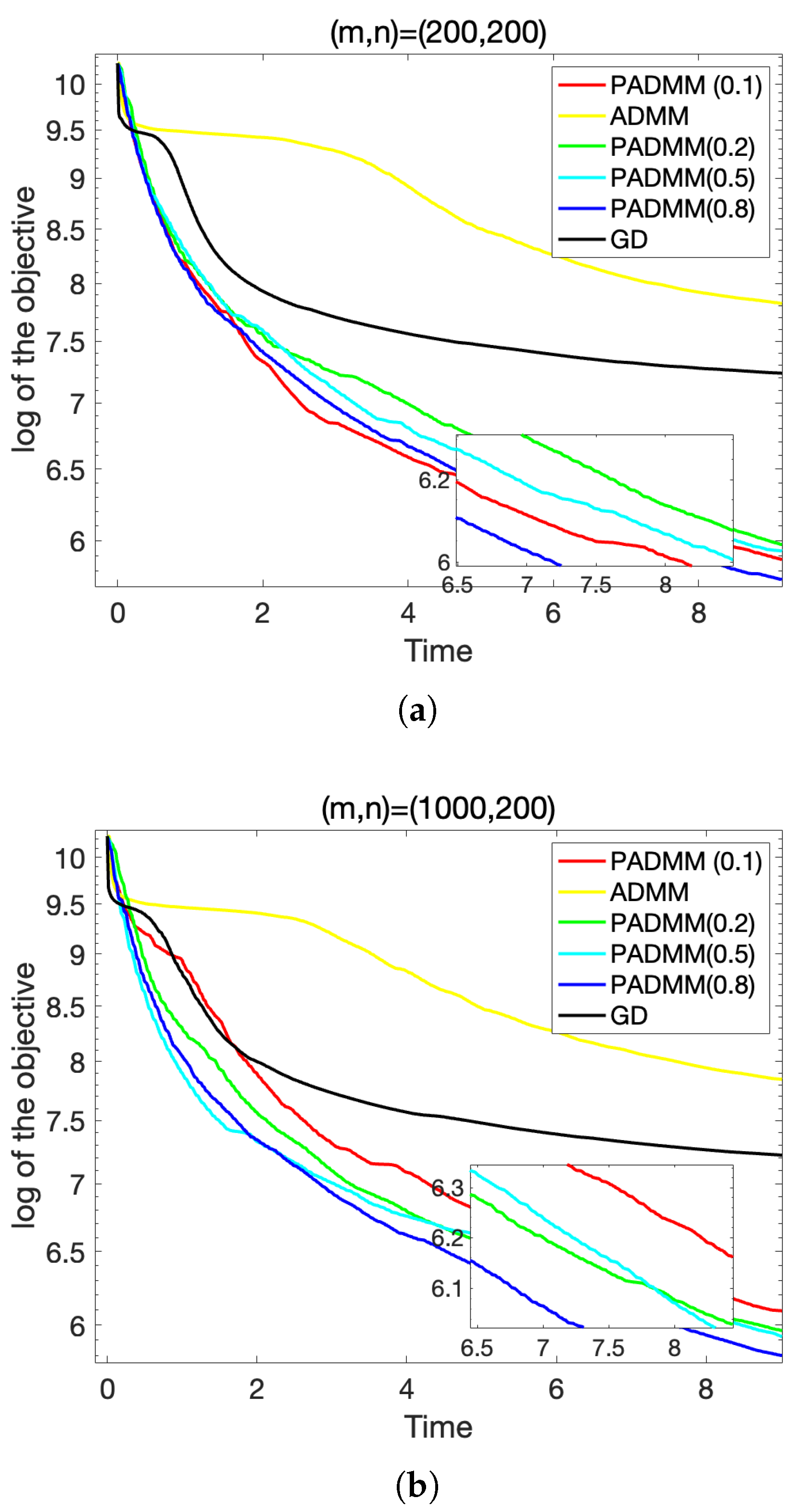
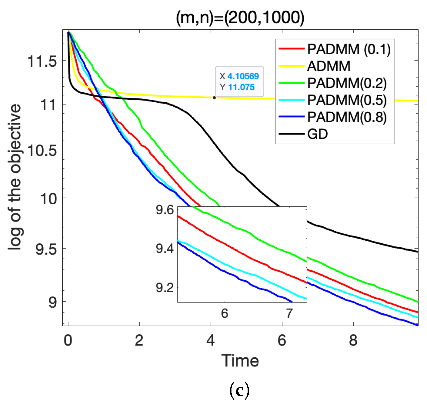
To generate sparse data $W\in {\mathbb{R}}^{m\times n}$, where each element $w_{ij}\in \{0,1\}$, we used the Matlab command sprand(m, n, s) and assigned them to W such that $W(W>0)=1$. In subsequent experiments, for each $(m,n)\in \left\{\right(200,200),(200,1000),(1000,200\left)\right\}$, we randomly generated a matrix Y and set $s=0.1$, meaning that 90% of the elements in Y were 0, with parameters $r=100,c=1,{\lambda }_d={\lambda }_t={\displaystyle \frac{1}{8}}$, and $\rho =1$. For each Y, we randomly generated initial points and ran each algorithm with the same initial points and running time. The running time for $(m,n)=(200,200)$ was set to 10 s, and for $(m,n)\in \left\{\right(200,1000),(1000,200\left)\right\}$, the running time was set to 20 s.

We conducted a comparative analysis of the proposed algorithm against two traditional methods: ADMM and the GD alternating gradient multiplier method. The GD alternating gradient multiplier method works by alternately updating matrices U and V using gradient descent steps. In our experiments, we evaluated the performance of the algorithm for different values of the regularization parameter $\tau$, specifically $\tau =0.1,0.2,0.5,0.8$.

To assess the performance of each method, we calculated the objective value of problem (3) throughout the iterations, and we present the change in this objective value over time in Figure 1 and

Table 1. Objective function value.

Algorithm/(m,n)	(200,200)	(1000,200)	(200,1000)
ADMM	7.4626 × 102	6.2803 × 103	6.3880 × 103
PADMM ($\tau =0.1$)	3.2967 × 102	4.8188 × 103	4.7594 × 103
PADMM ($\tau =0.2$)	3.6218 × 102	5.1283 × 103	4.6801 × 103
PADMM ($\tau =0.5$)	3.4799 × 102	4.7661 × 103	4.4719 × 103
PADMM ($\tau =0.8$)	3.6689 × 103	4.7492 × 103	4.2894 × 103
GD	4.5551 × 102	5.5551 × 103	5.4918 × 103

. The experimental results clearly show that the proposed algorithm consistently outperforms both the ADMM and GD alternating gradient multiplier methods on all values tested of $\tau$.

In particular, we observe that for $\tau =0.8$, the proposed algorithm achieves the best performance, with the objective value converging more rapidly and reaching a lower final value compared to the other methods. This suggests that the choice of $\tau$ plays a crucial role in optimizing the algorithm’s performance. Based on the experimental findings, we conclude that $\tau =0.8$ provides the optimal balance between efficiency and accuracy, making it the most effective choice for solving the problem at hand. This was also validated in subsequent experiments with real-world data.

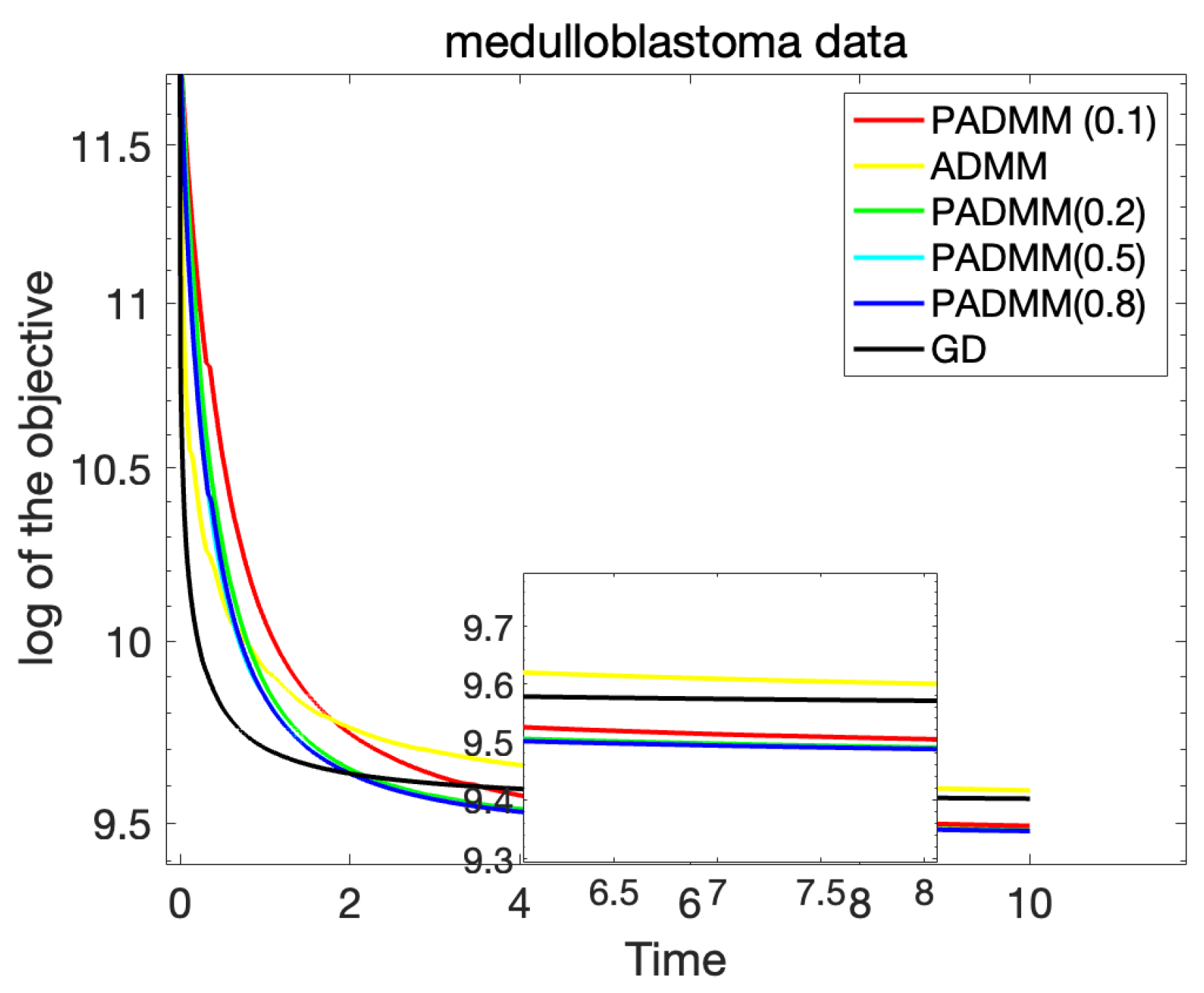
Similarly, we applied the proposed algorithm to a dataset containing medulloblastoma matrix data [20] and a real-world biomedical dataset and analyzed several key factors, including the relationship between the training values and the number of iterations, as well as the difference between the training value and the optimal value. This allowed us to evaluate how effectively the algorithm converges and whether it consistently approaches the optimal solution.

In Figure 2, we present the results of this analysis, which clearly highlight the superior performance of the PADMM algorithm in addressing real-world problems, particularly in the context of complex medical data. The graph shows that the proposed algorithm converges quickly and accurately, maintaining a small gap between the training value and the optimal value over time.

From these results, we can further conclude that, similarly to our earlier experiments, the regularization parameter $\tau =0.8$ delivers the best performance in this real-world scenario as well. The results validate the robustness and efficiency of the proposed algorithm, confirming that it can effectively handle practical, large-scale datasets while providing high accuracy and fast convergence.

5. Conclusions

We present a proximal linear alternating direction multiplier method for solving nonconvex, nonsmooth optimization problems with nonlinear coupling constraints. In this problem, the differentiable parts of the objective and constraints have locally Lipschitz continuous gradients. Our algorithm provides an alternating direction multiplier method for problem (1) that updates the variables using a linearized proximal technique and updates the dual variables through a discounting approach. By fixing the parameter selection, the algorithm does not require an additional proxy function or parameter adjustments to ensure the monotonicity of the generated sequence, and numerical experiments were conducted to demonstrate its effectiveness.