Article

Flow Shop Scheduling with Shortening Jobs for Makespan Minimization

1
School of Computer, Shenyang Aerospace University, Shenyang 110136, China
2
School of Mechatronics Engineering, Shenyang Aerospace University, Shenyang 110136, China
3
Key Laboratory of Rapid Development & Manufacturing Technology for Aircraft, Shenyang Aerospace University, Ministry of Education, Shenyang 110136, China
4
School of Mathematics and Computer, Shantou University, Shantou 515063, China
*
Authors to whom correspondence should be addressed.
These authors contributed equally to this work.
Mathematics 2025, 13(3), 363; https://doi.org/10.3390/math13030363
Submission received: 26 December 2024 / Revised: 15 January 2025 / Accepted: 21 January 2025 / Published: 23 January 2025

Abstract

:
This paper deals with a two-machine flow shop problem with shortening jobs. A shortening job means that the job’s processing time is a decreasing function of its starting time. The aim is to find a sequence that minimizes the makespan of all the jobs. several dominance properties, some lower bounds, and an initial upper bound are derived, which are applied to propose a branch-and-bound algorithm to solve the problem. We also propose some heuristics and mathematical programming. Computational experiments are conducted to evaluate the performance of the proposed algorithms.

1. Introduction

In scheduling theory, situations in which the job processing times increase or decrease compared with the starting time are often encountered, i.e., time-dependent processing times (denoted as T D P T s) (Strusevich and Rustogi [1], Gawiejnowicz [2], and Lee et al. [3]). The shortening of the processing time can effectively improve the efficiency of the work and reduce the consumption of resources, which is essential in industry. Generally, there are two models that are used to describe the T D P T . The first type concerns cases where the job processing time is a non-decreasing function of the starting time, i.e., a deteriorating job D e t e r J (Huang and Wang [4], Miao [5] Sun and Geng [6], Liu et al. [7], and Huang [8]). The second type is the case where the job processing time is a non-increasing function of the starting time, i.e., a shortening job (denoted by S h o r J , as shown in Ho et al. [9], Ng et al. [10], Bachman et al. [11]).
More recently, Qian and Zhan [12], Miao et al. [13], Qian and Han [14], and Lu et al. [15] considered the single-machine delivery time scheduling problems with D e t e r J . Using due date assignment, Qian and Zhan [12] proved that some problems can be solved in polynomial time. Considering release dates, Miao et al. [13] proved that some problems are NP-hard. With due window assignment, Qian and Han [14] and Lu et al. [15] proved that some problems can be solved in polynomial time. Sun et al. [16] studied single-machine maintenance activity scheduling with D e t e r J ; the corresponding solution algorithms (the parts that coul be solved in polynomial time, using branch-and-bound for the parts that could not be solved as well as heuristic algorithms) were also proposed for the studied elements. Atsmony and Mosheiov [17] explored single-machine total completion time minimization with D e t e r J ; the computational complexity of this problem remains an open problem. Qiu and Wang [18] studied single-machine scheduling with due window assignment and D e t e r J . Wang et al.  [19] conducted single-machine controllable processing time scheduling with D e t e r J . Li et al. [20] addressed two-agent single-machine scheduling with resource allocation, slack due date assignment, and general D e t e r J . Yin and Gao [21] studied single-machine group scheduling with a general D e t e r J and learning effects. None of the above-mentioned studies (Wang et al.  [19], Li et al. [20], Yin and Gao [21]) solved the problem in polynomial time. Wang et al. [22] considered single-machine group scheduling with S h o r J , subject to makespan minimization. The former can be solved in polynomial time for a given number of groups, while the latter considers the more general case, which has no exact solution algorithm. Obviously, there are fewer studies on S h o r J -type T D P T scheduling problems; thus, this paper fills the gap regarding such problems from this perspective.
For flow shop scheduling (Kovalev et al. [23] and Panwalkar and Koulamas  [24]) with T D P T , Kononov and Gawiejnowicz [25] and Mosheiov [26] considered computational complexity flow shop scheduling with D e t e r J , where the goal was to minimize the makespan. Lee et al. [27] (resp. Lee et al. [28]) studied two-machine flow shop problems with D e t e r J subject to makespan (resp. total completion time) minimization. Yin and Kang [29] considered some dominant relationships in flow shop problems with D e t e r J . Wang et al. [30] studied a flow shop problem with D e t e r J . For total tardy time minimization, they proposed an effective metaheuristic algorithm. Shabtay and Mor  [31] considered proportionate flow shop scheduling with step- D e t e r J . For makespan and total load minimizations, they proposed exact algorithms and approximation schemes. Wang and Wang [32] delved into flow shop scheduling with S h o r J . Under two-machine and total weighted completion time minimization, they proposed a branch-and-bound algorithm and two heuristics. Wang et al. [33] considered three-machine flow shop scheduling with S h o r J subject to makespan minimization. S h o r J has been less studied in standalone scheduling and even less in flow shops. Therefore, this paper combines S h o r J with flow shop settings and discusses the special case of two machines.
Due to the limited exploration of flow shop settings with S h o r J , in this paper, we tackle two-machine flow shop scheduling with S h o r J , where the shortening rates of all jobs are identical. For makespan minimization, we present a branch-and-bound algorithm and some heuristic algorithms. The main contributions of this paper are as follows: (i) flow shop scheduling with S h o r J is studied and simulated with data; (ii) for a given schedule, the optimal solution properties are given; (iii) for the problem of makespan minimization, we analyze the lower bound of the problem, design a branch-and-bound algorithm and several heuristic algorithms to solve the problem, and verify the performance of each algorithm through computational experiments. The rest of this paper is organized as follows: In Section 2, we describe the problem. In Section 3, we propose the branch-and-bound algorithm, some heuristic algorithms, and mathematical programming. In Section 4, we present the results of computational experiments. In Section 5, we conclude this paper.

2. Problem Formulation

Let N = { J 1 , J 2 , , J n } be a set of jobs to be processed in a 2-machine flow shop, where the set of 2 machines is M = { M 1 , M 2 } . All jobs have the same processing order through the machines and are ready for processing at time t 0 0 . Let p i j be the actual processing time of J j   ( j = 1 , 2 , , n ) on   M i ( i = 1 , 2 ) (i.e., operation O i j ) if it is started at time t. For the general model, the actual processing time of operation O i j is p i j = ϑ i j λ i j t , where ϑ i j (resp. λ i j ) is the normal processing time (resp. shortening rate). As in Cheng et al. [34], we consider the S h o r J model
p i j = ϑ i j λ t ,
where λ 0 is the identical shortening rate for all the jobs, λ satisfies 0 < λ < 1 , and in order to ensure that the actual processing time of any job is greater than 0, λ also needs to satisfy λ ( t 0 + i = 1 n j = 1 n ϑ i j ϑ min ) < 1 , where ϑ min = min i = 1 , 2 ; j = 1 , 2 , , n { ϑ i j } .
Let C i , j ( π ) be the completion time of J j on M i under some sequence π . Thus, the completion time of J j is C j = C 2 , j . The aim is to minimize the makespan; the problem can be denoted as F 2 | p i j = ϑ i j λ t | C max . Table 1 presents the flow shop research results related to this study.

3. Solution Algorithms

Simply, ϑ 1 j (resp. ϑ 2 j ) is denogted by α j (resp. β j ). Obviously, fothe machine M 1 , we have
C 1 , 1 = t 0 + α 1 λ t 0 = α 1 + 1 λ t 0 , C 1 , 2 = C 1 , 1 + α 2 λ C 1 , 1 = α 2 + 1 λ α 1 + 1 λ 2 t 0 ;
thus, for the jth in M 1 , we can obtain the following equation:
C 1 , [ j ] = t 0 ( 1 λ ) j + i = 1 j α [ i ] ( 1 λ ) j i , j = 1 , 2 , , n .
For problem F 2 | p i j = ϑ i j λ t | C max , we conjecture that its computational complexity is NP-hard; hence, some solution algorithms (including the branch-and-bound and heuristic algorithms) are proposed to solve this problem.

3.1. Dominance Properties

Given S 1 = ( π , J j , J i , π ) and S 2 = ( π , J i , J j , π ) , where π and π are partial sequences, and there are r 1 jobs in π . Let E (resp. F) be the completion time of the last job in π on M 1 (resp. M 2 ). To show that S 2 dominates S 1 , it suffices to show that C j ( S 2 ) C i ( S 1 ) (i.e., C [ h ] ( S 2 ) C [ h ] ( S 1 ) , h = r + 1 , r + 2 , , n , where C [ h ] denotes the completion time of the hth job).
Proposition 1.
It is supposed that two jobs J i and J j satisfy the following conditions:
(i) 
Either ( α i α j ) ( 1 λ ) 2 λ ( β i β j ) or β j λ β i α j ( 1 λ ) 2 λ ( 1 λ ) α i or E ( 1 λ ) 3 + α i ( 1 λ ) 2 F ( 1 λ ) 2 + λ ( β i β j ) ;
(ii) 
Either α i ( 1 λ ) 2 + λ ( 1 λ ) α j β i λ β j or λ ( 1 λ ) ( α j α i ) β i β j or E ( 1 λ ) 3 + α i ( 1 λ ) 2 + α j ( 1 λ ) F ( 1 λ ) 2 + β i λ β j ;
(iii) 
Either F ( 1 λ ) 2 + λ ( β j β i ) E ( 1 λ ) 3 + α j ( 1 λ ) 2 or F ( 1 λ ) 2 + β j λ β i E ( 1 λ ) 3 + α j ( 1 λ ) 2 + α i ( 1 λ ) or β j β i .
Then, S 2 dominates S 1 .
Proof. 
See Appendix A.    □

3.2. Lower Bounds

Lemma 1
(Hardy et al. [35]). j = 1 n x j y j is minimized if x 1 , x 2 , , x n (resp. y 1 , y 2 , , y n ) is ordered non-decreasingly (resp. non-increasingly) or vice versa.
Suppose S = ( π P S , π ) , where π P S (resp. π ) is a partial schedule that has (resp. not) been sorted, and there are k jobs in π P S . Let A be the completion time of the kth job on M 1 . We have
C [ k + 1 ] ( S ) = ( 1 λ ) max { ( 1 λ ) A + α [ k + 1 ] , C [ k ] ( S ) } + β [ k + 1 ] ( 1 λ ) 2 A + ( 1 λ ) α [ k + 1 ] + β [ k + 1 ] .
Similarly, for the nth job, we have
C [ n ] ( S ) ( 1 λ ) n k + 1 A + i = k + 1 n ( 1 λ ) n i + 1 α [ i ] + β [ n ] .
It can be noticed that ( 1 λ ) n k + 1 A is fixed, and ( 1 λ ) n i + 1 is a increasing function of i; thus, i = k + 1 n ( 1 λ ) n i + 1 α [ i ] is minimized by the non-increasing order of α i through Lemma 1, and β [ n ] is minimized by min i π β i ; hence, the first lower bound is
L B 1 = ( 1 λ ) n k + 1 A + i = k + 1 n ( 1 λ ) n i + 1 α ( i ) + min i π β i ,
where α ( k + 1 ) α ( k + 2 ) α ( n ) . In addition, we have
C [ k + 1 ] ( S ) = ( 1 λ ) max { ( 1 λ ) A + α [ k + 1 ] , C [ k ] ( S ) } + β [ k + 1 ] ( 1 λ ) C [ k ] ( S ) + β [ k + 1 ]
and
C [ n ] ( S ) ( 1 λ ) n k C [ k ] ( S ) + i = k + 1 n ( 1 λ ) n i β [ i ] .
Note that ( 1 λ ) n k C [ k ] ( S ) is fixed; similarly, the second lower bound is
L B 2 = ( 1 λ ) n k C [ k ] ( S ) + i = k + 1 n ( 1 λ ) n i β ( i ) ,
where β ( k + 1 ) β ( k + 2 ) β ( n ) .
Adding (3) and (5) yields
C [ n ] ( S ) 1 2 ( 1 λ ) n k + 1 A + β [ n ] + ( 1 λ ) n k C [ k ] ( S ) + i = k + 1 n ( 1 λ ) n i + 1 ( α [ i ] + β [ i ] ) .
Note that ( 1 λ ) n k + 1 A + ( 1 λ ) n k C [ k ] ( S ) is fixed; similarly, the third lower bound is
L B 3 = 1 2 ( 1 λ ) n k + 1 A + ( 1 λ ) n k C [ k ] ( S ) + min i π β i + i = k + 1 n ( 1 λ ) n i + 1 ( α ( i ) + β ( i ) ) ,
where α ( k + 1 ) + β ( k + 1 ) α ( k + 2 ) + β ( k + 2 ) α ( n ) + β ( n ) .
From the maximum value of (4), (6), and (8), the tighter lower bound is
L B = max { L B 1 , L B 2 , L B 3 } .

3.3. Heuristic Algorithms

It is well known that the Johnson solution provides the optimal solution to F 2 | p i j = ϑ i j | C max (i.e., λ = 0  [36]), hence the first heuristic algorithm is Johnson solution (denoted by J S ). In addition, by the calculation procedure of the lower bound, the second (resp. third, fourth) heuristic algorithm is: Sort all the jobs in non-decreasing order of α j (resp. β j , α j + β j ), and this heuristic algorithm can be denoted as L P T 1 ( L P T 2 , L P T 1 + 2 
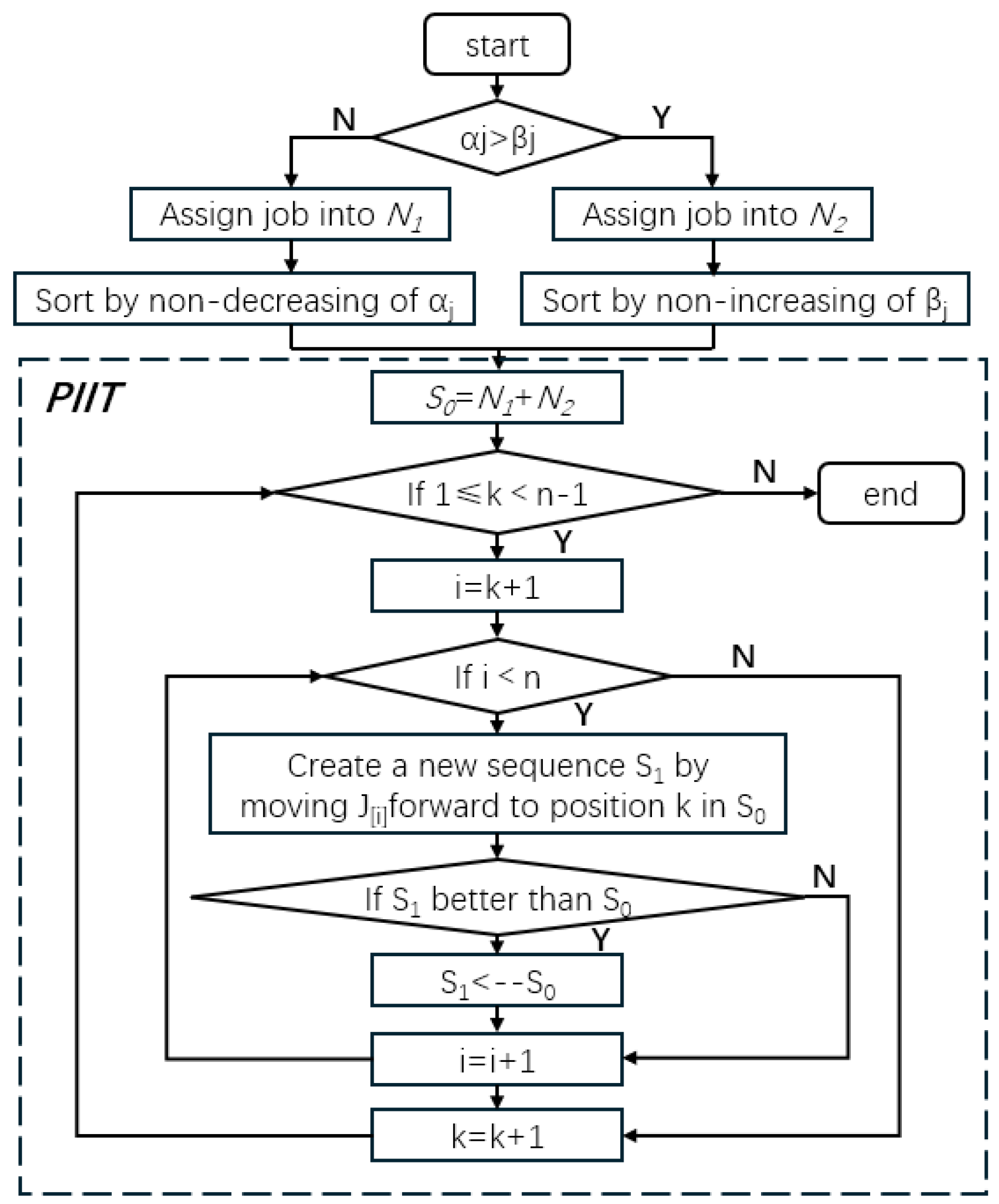
). All these heuristic algorithms are further improved by pairwise interchange technology, the flowchart of Algorithm 1 is shown in Figure 1, and these heuristic algorithms can be given as follows:
Algorithm 1:  J S .
  • Step 1. Partition the set of jobs N = { J 1 , J 2 , , J n } into two subsets N 1 = { J j | α j β j } and N 2 = { J j | α j > β j } .
  • Step 2. Order the jobs of N 1 (resp. N 2 ) in non-decreasing (resp. non-increasing) order of α j (resp. β j ), and the ordered jobs N 1 precede the order of N 2 .
  • Step 3. Let S 0 be the schedule obtained from Steps 1 and 2.
  • Step 4. Set k = 1 and i = k + 1 .
  • Step 5. Create a new sequence S 1 by moving J [ i ] forward to position k in S 0 . Replace S 0 with S 1 if the makespan value of S 1 is smaller than that of S 0 .
  • Step 6. If i < n , set i = i + 1 , and go to Step 5.
  • Step 7. If k < n 1 , set k = k + 1 , and go to Step 4. Otherwise, stop. Steps 3–7 describe the pairwise interchange improvement technology, denoted by P I I T )
Theorem 1.
The time complexity of Algorithm 1 is O ( n 2 ) .
Proof. 
Partition all jobs into two subsets N 1 and N 2 ; this step needs O ( n ) time. Then, the jobs in N 1 and N 2 are sorted, and the time complexity of this operation is O ( n log n ) . P I I T contains two layers of loops from 1 to n, so the time complexity of P I I T is O ( n 2 ) . The overall time complexity of Algorithm 1 is determined by the part with the highest complexity among the above steps, so the time complexity of Algorithm 1 is O ( n 2 ) .    □
Theorem 2.
The time complexity of Algorithms 2–4 is O ( n 2 ) .
Algorithm 2:  L P T 1 .
  • Step 1. Arrange the jobs in non-increasing order of α j to obtain an initial schedule.
  • Step 2. Use P I I T .
Algorithm 3:  L P T 2 .
  • Step 1. Arrange the jobs in non-increasing order of β j to obtain an initial schedule.
  • Step 2. Use P I I T .
Algorithm 4:  L P T 1 + 2 .
  • Step 1. Arrange the jobs in non-increasing order of α j + β j to obtain an initial schedule.
  • Step 2. Use P I I T .
Proof. 
This proof is similar to the proof for Theorem 1.    □

3.4. Tabu Search

In order to compare the above proposed heuristic with others, the same tabu search algorithm with a wide range of applications in scheduling problems was used. From Glover and Laguna [37], the tabu search Algorithm 5 is proposed to solve F 2 | p i j = ϑ i j λ t | C max , where an initial sequence can be obtained by J S , and the maximum number of iterations is equal to 100 n (Wu et al. [38], Lv and Wang  [39] and Liu and Wang  [40]).
Algorithm 5:  T S .
  • Step 1. Let the tabu list be empty and the iteration number be zero.
  • Step 2. Set the initial sequence of Algorithm 5, calculate the makespan, and set the current schedule as the best solution S 0 .
  • Step 3. Search the associated neighborhood of the current sequence and resolve it if there is a sequence S 1 with the smallest makespan in the associated neighborhood and it is not in the tabu list.
  • Step 4. If S 1 is better than S 0 , let S 0 = S 1 . Update the tabu list and the iteration number.
  • Step 5. If there is no sequence in the associated neighborhood but it is not in the tabu list or the maximum number of iterations is reached, output the final sequence. Otherwise, update the tabu list and go to Step 3.

3.5. The Branch-And-Bound Algorithm

From Section 3.1, Section 3.2 and Section 3.3, we present a branch-and-bound (denoted by b-a-b) Algorithm 6 to solve F 2 | p i j = ϑ i j λ t | C max .
Algorithm 6: b-a-b.
  • Step 1. Initialization: An initial upper bound (sequence) is obtained by choosing a better sequence from J S , L P T 1 , L P T 2 , and L P T 1 + 2 .
  • Step 2. Fathoming: Proposition 1 is used to eliminate the dominated partial sequences from the initial node and their descendants from the tree.
  • Step 3. Bounding: Calculate the lower bound (by using (9)) for the node. If the lower bound for an unfathomed partial schedule is larger than or equal to the value of the makespan of the initial solution, eliminate the node and all the nodes following it in the branch. Calculate the makespan of the completed sequence: if it is less than the initial solution, replace it as the new solution; otherwise, eliminate it.
  • Step 4. Termination: Continue until all nodes have been explored.
To verify the accuracy of the aforementioned b-a-b algorithm and the effectiveness of the lower bounds in solving problem F 2 | p i j = ϑ i j λ t | C max , an example is given in this subsection. Consider the example of n = 6 , t 0 = 1 , and b = 0.5 G , where G = 1 / [ i = 1 n ( α i + β i ) min i = 1 , 2 , , n { α i , β i } ] , and other data of the jobs are given in Table 2.
According to the data in Table 1, the parameter λ can be given as λ = 0.5 / [ i = 1 6 ( α i + β i ) min i = 1 , 2 , , 6 { α i , β i } ] = 0.004348 . 
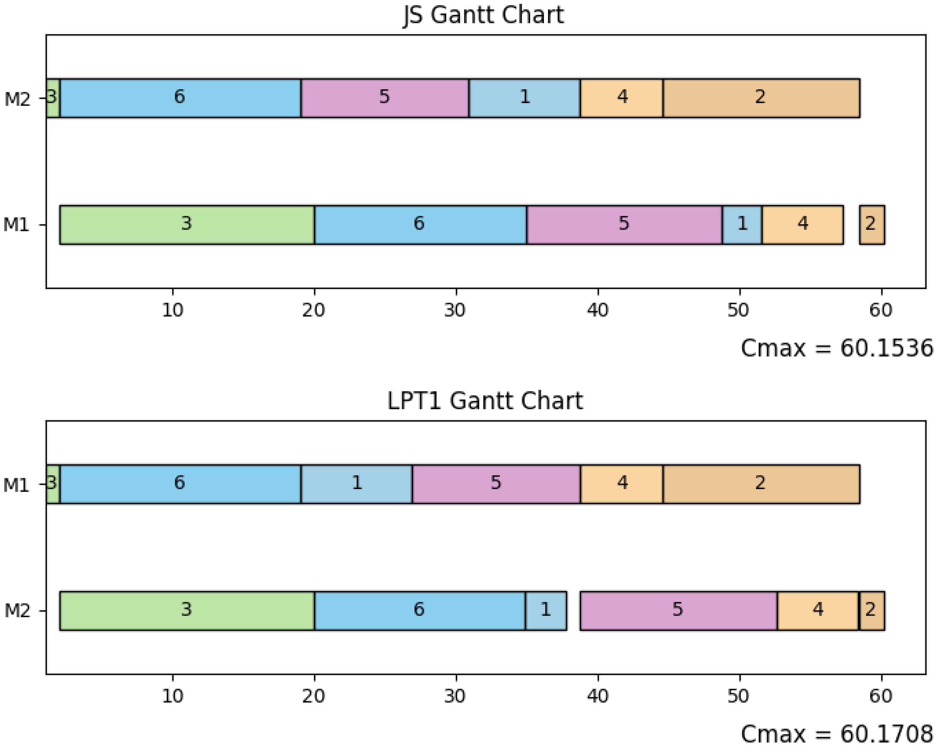
Figure 2 shows that the initial schedule produced by Algorithms 1 and 3 is J 3 J 6 J 5 J 1 J 4 J 2 , with a corresponding objective function value of 60.1536. The detailed steps of the b-a-b algorithm are outlined below. Once the processing sequence J 1 is fixed, the lower bound is determined as L B = max L B 1 , L B 2 , L B 3 = 66.0455 by comparing Equations (4), (6) and (8) (other lower bounds are derived following a similar method):
L B 1 = ( 1 λ ) n k + 1 A + i = k + 1 n ( 1 λ ) n i + 1 α ( i ) + min i π β i = 1 0.004348 6 × 8.9957 + 1 0.004348 5 × 17 + 1 0.004348 4 × 14 + 1 0.004348 3 × 12 + 1 0.004348 2 × 6 + 1 0.004348 1 × 1 + 2 = 59.943
L B 2 = ( 1 λ ) n k C [ k ] ( S ) + i = k + 1 n ( 1 λ ) n i β ( i ) = 1 0.004348 5 × 11.9565 + 1 0.004348 4 × 18 + 1 0.004348 3 × 15 + 1 0.004348 2 × 14 + 1 0.004348 1 × 6 + 1 0.004348 0 × 2 = 66.0455
L B 3 = 1 2 ( 1 λ ) n k + 1 A + ( 1 λ ) n k C [ k ] ( S ) + min i π β i + i = k + 1 n ( 1 λ ) n i + 1 ( α ( i ) + β ( i ) ) = 1 2 1 0.004348 6 × 8.9957 + 1 0.004348 5 × 11.9565 + 2 + 1 0.004348 5 × 17 + 15 + 1 0.004348 4 × ( 12 + 14 ) + 1 0.004348 3 × ( 1 + 18 ) + 1 0.004348 2 × ( 14 + 2 ) + 1 0.004348 1 × ( 6 + 6 ) ) = 62.9429
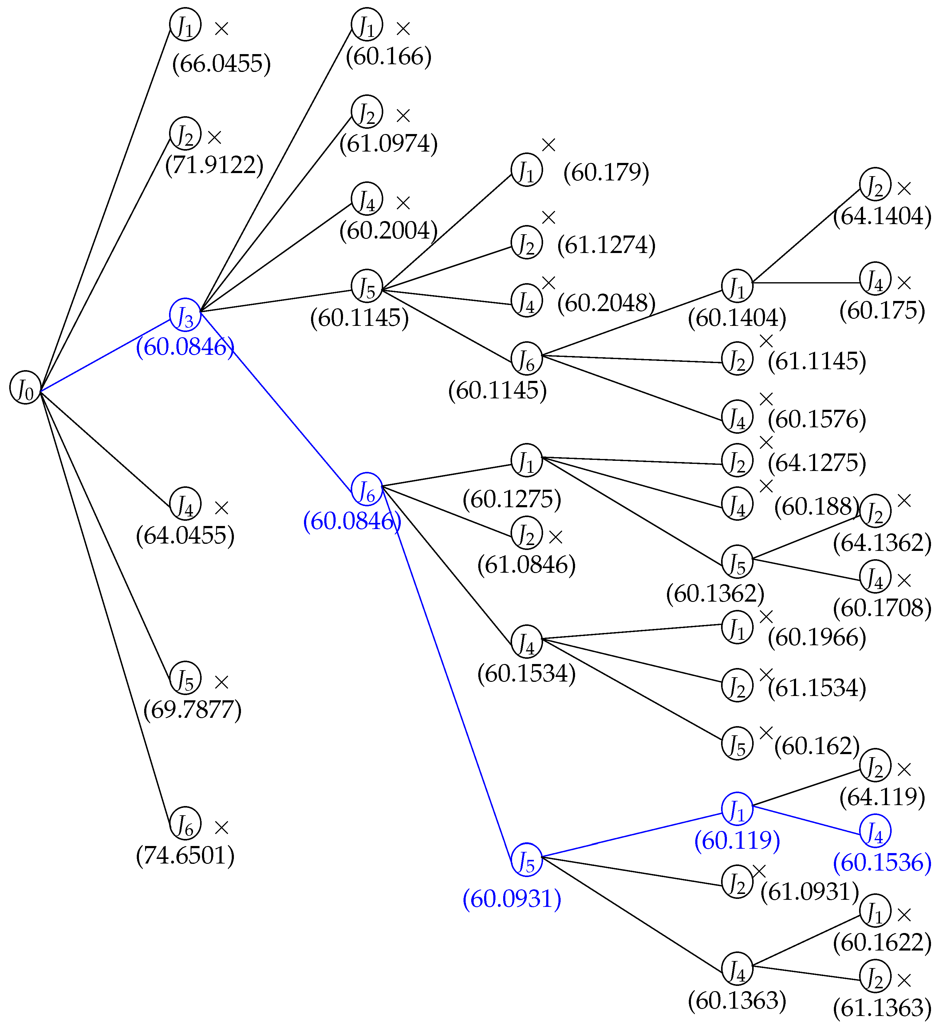
From the b-a-b tree (see Figure 3), it can be concluded that the optimal schedule is J 3 J 6 J 5 J 1 J 4 J 2 , with a corresponding objective function value of 60.1536. In this process, the b-a-b algorithm explores a total of 39 nodes.

3.6. Mathematical Programming Model

In this subsection, we design a mathematical programming model for solving F 2 | p i j = ϑ i j λ t | C max . The specific model is described as follows:
Min C max = C [ n ]
s . t . j = 1 n X j k = 1 , k = 1 , 2 , . . . , n
k = 1 n X j k = 1 , j = 1 , 2 , . . . , n
α k = j = 1 n X j k α j , k = 1 , 2 , . . . , n
β k = j = 1 n X j k β j , k = 1 , 2 , . . . , n
S 1 k = t 0 , k = 1
S 1 k C 1 k 1 , k = 2 , . . . , n
C 1 k α k + 1 λ S 1 k , k = 1 , 2 , . . . , n
S k C 1 k , k = 1 , 2 , . . . , n
S k C k 1 , k = 1 , 2 , . . . , n
C k β k + 1 λ S k , k = 1 , 2 , . . . , n
where X j k = 1 , i f j o b J j i s a s s i g n e d t o p o s i t i o n k ; 0 , o t h e r w i s e , S 1 k (resp. C 1 k ) indicates the start time (resp. completion time) of J [ k ] on M 1 , and S k (resp. C k ) indicates the start time (resp. completion time) of J [ k ] on M 2 . Equation (10) is the objective cost of optimization, Constraint (11) ensures that each job is placed in a unique position, Constraint (12) ensures that each position has only one unique job, and Constraints (13) and (14), respectively, indicate the normal processing time of the job at the kth position on M 1 and the normal processing time of the job at the kth position on M 2 . Constraints (15) and (16) indicate that the start time of the job on M 1 is no earlier than t 0 and the completion time of the previous job; Constraint (17) indicates that the completion time of the job at the kth position on M 1 is not less than the sum of its start processing time and actual processing time. Constraints (18) and (19) indicate that the start time of the kth job on M 2 is not earlier than the completion time of the kth job on M 1 nor earlier than the completion time of the ( k 1 ) th job on M 2 ; constraint (20) represents that the completion time of the job at the kth position on M 2 is not less than the sum of its start processing time and actual processing time.

4. Computational Experiments

We conducted computational experiments to evaluate the effectiveness of the b-a-b algorithm and the heuristic algorithms (i.e., Algorithms 1–6). We coded these algorithms in Visual studio2022 v17.1.0 and ran the computational experiments on a desktop work station with a CPU with a 12th Gen Intel(R) Core(TM) i5-12400 2.50 GHz, 16.00 GB RAM, and a Windows 11 operating system.
For the purpose of experimentation, the subsequent parameters were defined to facilitate the random generation of test instances:
(1)
Small-scale number of jobs n = 5, 6, 7, 8, 9, 10, 11, 12, 13, 14, 15, 16, 17, 18, 19 and 20;
(2)
Large-scale number of jobs n = 50, 60, 70, 80, 90, 100, 110, 120, 130, 140, 150, 160, 170, 180, 190 and 200 (b-a-b algorithm was disabled);
(3)
α j and β j were sampled from uniform discrete values distributed over [1, 100];
(4)
t 0 = 1 , λ = 0.5 G , and λ = 0.1 G were used, where G = 1 / [ i = 1 n ( α i + β i ) min i = 1 , 2 , , n { α i , β i } ] .
For the purpose of assessing the b-a-b algorithm, sixteen different numbers of jobs within the small-scale range were employed in the experimentation; for each parameter combination, 20 test instances were randomly generated; and the average (maximum) number of nodes and CPU time (in millisecond, ms) are reported. For the heuristic algorithms, the recorded metrics included the average (maximum) errors and CPU times, where the error was calculated as
C max ( H e u ) C max ( O p ) C max ( O p ) ,
in which H e u { J S , L P T 1 , L P T 2 , L P T 1 + 2 , T S } , C max ( H e u ) is the makespan value of the heuristic algorithm, and C max ( O p ) is the optimal makespan value of the b-a-b algorithm. The results are summarized in Table 3, Table 4, Table 5 and Table 6 and Figure 4.
The analysis of Table 3 and Table 4 shows that there was a positive correlation between the execution time and the number of nodes, and both metrics increase with the value of λ . In addition, the branch-and-bound algorithm was able to solve problems with job sizes less than or equal to 20 within a reasonable time frame. However, the execution time and the number of nodes increased dramatically as the job size increased since we considered an NP-hard problem. From Table 3, Table 4, Table 5 and Table 6 and Figure 4, the most time-consuming case of the branch-and-bound algorithm took about 1,825,642.35 ms. In the heuristic approach, for instance, when λ = 0.1 G (the case for λ = 0.5 G is analogous), Algorithms 1, 3, and 5 exhibited comparable accuracy, with average error rates of 0.0013, 0.0026, and 0.0010, respectively. However, the T S algorithm demonstrated a markedly longer computational time compared to Algorithms 1 and 3, with average run times (in milliseconds) of 533.82, 0.25, and 0.24, respectively. From Table 3 and Table 4, we can see that the average CPU time of all heuristics except the T S algorithm was less than 1 ms, and the maximum time did not exceed 3 ms. Table 5 and Table 6 show the error rate information for each heuristic algorithm for the small scale. We can see that the average error rate of all algorithms did not exceed 1%, and the maximum error rate did not exceed 5%. By looking at 
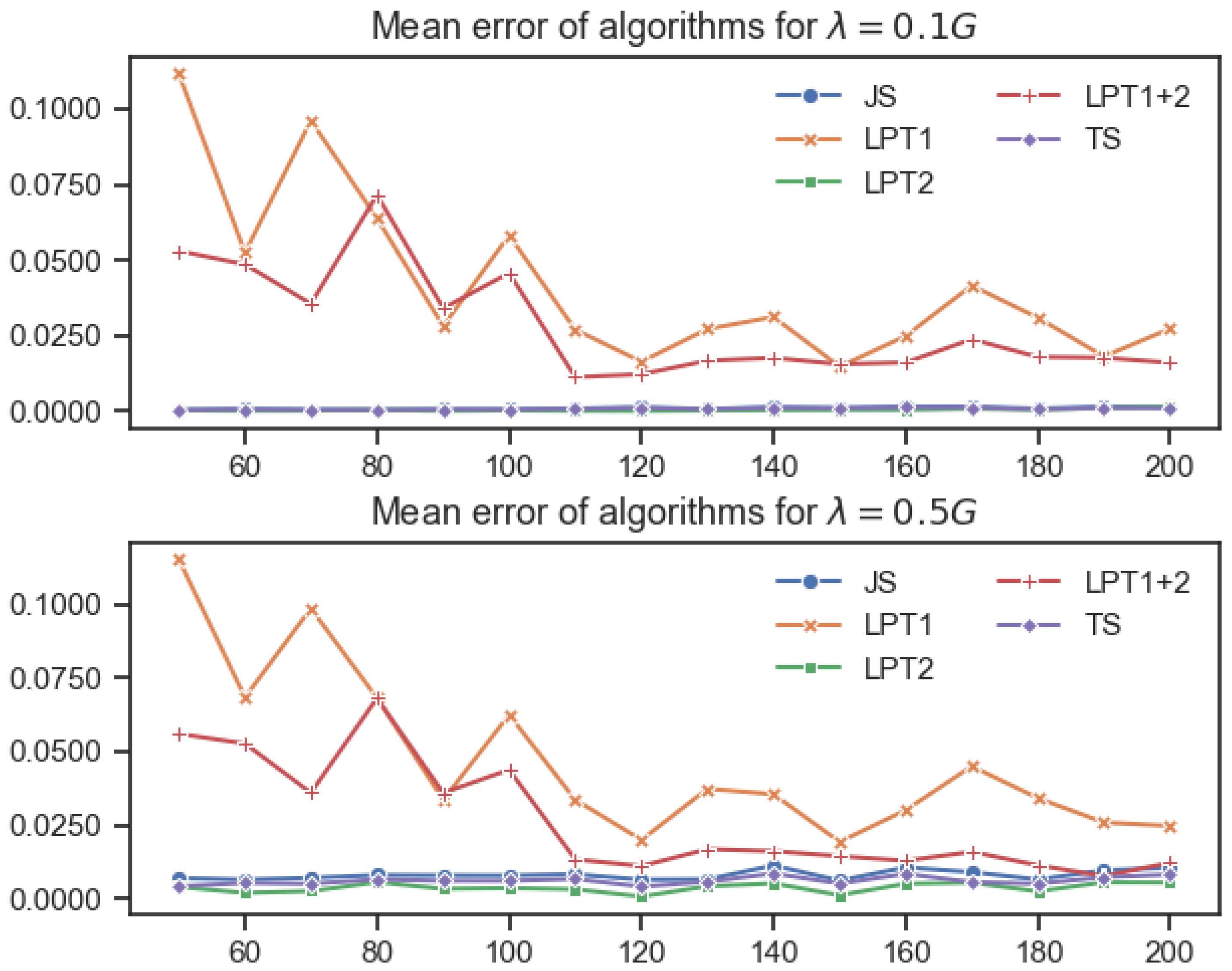
Figure 4, we can intuitively conclude that the stability of Algorithms 1, 3 and 5 was significantly better than the other two algorithms.
The computational experiments on a large scale were similar to the small scale, and the results of the experiments are displayed in Table 7, Table 8, Table 9 and Table 10 and Figure 5. At the small scale, it can be seen from Table 3 and Table 4 that the CPU time of the b-a-b algorithm increased dramatically with the increase in the number of jobs, and the number of nodes that needed to be traversed also increased sharply. Although the optimal solution to the problem could be found in large-scale cases, the CPU time required was extremely long and unacceptable. Therefore, in the large-scale cases, we mainly verified the performance of the heuristic algorithms. The error rate at the large scale was also computed in a similar way to that at the small scale, except that Opt represented the best solution in the heuristic algorithm and not necessarily the optimal solution to the problem. From the experimental results, it is evident that the accuracy and stability of Algorithms 1, 3 and 5 were significantly superior to those of L P T 1 and L P T 1 + 2 . For instance, when λ = 0.1 G , the average error rates for the five algorithms were as follows: J S : 0.00098 , L P T 1 : 0.04185 , L P T 2 : 0.00045 , L P T 1 + 2 : 0.02834 , and T S : 0.00080 . However, the running time of Algorithm 5 was significantly higher than the other heuristic algorithms. It can be seen from Table 7 and Table 9 that the running efficiencies of each heuristic algorithm were acceptable. Although the running time of the TS algorithm was longer than that of the other four heuristic algorithms, the maximum running time did not exceed 300,115.19 ms, which is acceptable. The maximum running times of the other four heuristic algorithms were quite similar, all around 7000 ms. Regarding the error rates of each algorithm, Table 8 and Table 10 show that the average error rates of these five algorithms were all no more than 0.11528%, and their maximum error rates were all no more than 1.05166%. Combined with Figure 4, it can be more intuitively concluded that as the number of jobs increased, the error rates of each algorithm decreased, but they were similar overall to those in the small-scale cases. The accuracy rates of Algorithms 1, 3 and 5 were significantly better than those of Algorithms 2 and 4. In summary, it can be seen that the results of the large-scale experiments were similar to those of the small-scale experiments, and the heuristic Algorithms 1 and 3 had the optimal performance in solving F 2 | p i j = ϑ i j λ t | C max .
To validate the efficacy of the b-a-b algorithm, we conducted computational experiments that compared it with the b-a-b algorithm and a mathematical programming model, specifically Equations (10)–(20), which were solved using Gurobi (Version 11.0.3). The experiment was conducted on the small scale (i.e., n = 10 , 11 , 12 , 13 , 14 , 15 ), and, for each combination of parameters, 10 random instances were generated. The experimental results are displayed in Table 11, which records the optimal object value obtained by Gurobi and the b-a-b algorithm and the CPU times (ms) of Gurobi and the b-a-b algorithm. Regarding the CPU time, when n 13 , the b-a-b algorithm was significantly better than Gurobi in 72 % of cases (i.e., 72 out of 100).

5. Conclusions

In this paper, two-machine flow shop makespan minimization with S h o r J was studied. Several dominance conditions, lower bounds, and an upper bound were derived and applied in a b-a-b algorithm. Some heuristic algorithms and mathematical programming were also proposed. This study enriches the research on scheduling theory with time-dependent processing times ( T D P T s), expands the research on the problem of shortening job processing times ( S h o r J ) in a two-machine flow shop, proposes multiple algorithms and related theoretical analyses, verifies the performance of the algorithms through computational experiments, provides guidance for practical production scheduling decisions, and offers references for research on similar scheduling problems in the future.
Through a large number of computational experiments, the performance of the proposed algorithms was verified. Although the running efficiency and accuracy of some heuristic algorithms were suitable in the experiments, there are many uncertain factors in real production, and these factors may interfere with the performance of the algorithms. In addition, some of the algorithms proposed in this paper are based on the nature of the problem studied, and it is unknown whether they are applicable to solving other scheduling problems. Further research may consider flow shop scheduling with learning effects (Sun et al. [41], and Zhang et al. [42]), or resource allocation ( Qian et al. [43], Qian and Guo [44], and Zhang et al. [45]). In addition, in the context of Industry 5.0, it would also be meaningful to study scheduling problems with energy constraints (see Wang and Wang [46]).

Author Contributions

Methodology, Z.-W.S.; Writing—original draft, Z.-W.S.; Writing—review & editing, Z.-W.S., D.-Y.L., C.-M.W. and J.-B.W. All authors have read and agreed to the published version of the manuscript.

Funding

This research was funded by the fundamental research funds for the universities of liaoning province (JYTMS20230278).

Data Availability Statement

The data used to support this paper are available from the corresponding author upon request.

Conflicts of Interest

The authors declare no conflicts of interest.

Appendix A. The Proof of Proposition 1

Proof. 
The completion times of J k in sequences S 1 and S 2 are equal if in π , i.e.,
C [ k ] ( S 1 ) = C [ k ] ( S 2 ) , if J [ k ] π .
Under S 2 , we have
C [ r ] ( S 2 ) = C i ( S 2 ) = max { E + α i λ E , F } + β i λ max { E + α i λ E , F } = max { E ( 1 λ ) 2 + α i ( 1 λ ) + β i , F ( 1 λ ) + β i } ,
and
C [ r + 1 ] ( S 2 ) = C j ( S 2 ) = max { E ( 1 λ ) 3 + α i ( 1 λ ) 2 + β i ( 1 λ ) + β j , E ( 1 λ ) 3 + α i ( 1 λ ) 2 + α j ( 1 λ ) + β j , F ( 1 λ ) 2 + β i ( 1 λ ) + β j } .
Under S 1 , we have
C [ r ] ( S 1 ) = C j ( S 1 ) = max { E ( 1 λ ) 2 + α j ( 1 λ ) + β j , F ( 1 λ ) + β j } ,
and
C [ r + 1 ] ( S 1 ) = C i ( S 1 ) = max { E ( 1 λ ) 3 + α j ( 1 λ ) 2 + β j ( 1 λ ) + β i , E ( 1 λ ) 3 + α j ( 1 λ ) 2 + α i ( 1 λ ) + β i , F ( 1 λ ) 2 + β j ( 1 λ ) + β i } .
From (A3) and (A5), we have
C [ r + 1 ] ( S 2 ) C [ r + 1 ] ( S 1 ) max { E ( 1 λ ) 3 + α i ( 1 λ ) 2 + β i ( 1 λ ) + β j , E ( 1 λ ) 3 + α i ( 1 λ ) 2 + α j ( 1 λ ) + β j , F ( 1 λ ) 2 + β i ( 1 λ ) + β j } max { E ( 1 λ ) 3 + α j ( 1 λ ) 2 + β j ( 1 λ ) + β i , E ( 1 λ ) 3 + α j ( 1 λ ) 2 + α i ( 1 λ ) + β i , F ( 1 λ ) 2 + β j ( 1 λ ) + β i } E ( 1 λ ) 3 + α i ( 1 λ ) 2 + β i ( 1 λ ) + β j max { E ( 1 λ ) 3 + α j ( 1 λ ) 2 + β j ( 1 λ ) + β i , E ( 1 λ ) 3 + α j ( 1 λ ) 2 + α i ( 1 λ ) + β i , F ( 1 λ ) 2 + β j ( 1 λ ) + β i } a n d E ( 1 λ ) 3 + α i ( 1 λ ) 2 + α j ( 1 λ ) + β j max { E ( 1 λ ) 3 + α j ( 1 λ ) 2 + β j ( 1 λ ) + β i , E ( 1 λ ) 3 + α j ( 1 λ ) 2 + α i ( 1 λ ) + β i , F ( 1 λ ) 2 + β j ( 1 λ ) + β i } a n d F ( 1 λ ) 2 + β i ( 1 λ ) + β j } max { E ( 1 λ ) 3 + α j ( 1 λ ) 2 + β j ( 1 λ ) + β i , E ( 1 λ ) 3 + α j ( 1 λ ) 2 + α i ( 1 λ ) + β i , F ( 1 λ ) 2 + β j ( 1 λ ) + β i } ( i ) E i t h e r ( α i α j ) ( 1 λ ) 2 λ ( β i β j ) o r β j λ β i α j ( 1 λ ) 2 λ ( 1 λ ) α i o r E ( 1 λ ) 3 + α i ( 1 λ ) 2 F ( 1 λ ) 2 + λ ( β i β j ) ; a n d ( i i ) E i t h e r α i ( 1 λ ) 2 + λ ( 1 λ ) α j β i λ β j o r λ ( 1 λ ) ( α j α i ) β i β j o r E ( 1 λ ) 3 + α i ( 1 λ ) 2 + α j ( 1 λ ) F ( 1 λ ) 2 + β i λ β j . a n d ( i i i ) E i t h e r F ( 1 λ ) 2 + λ ( β j β i ) E ( 1 λ ) 3 + α j ( 1 λ ) 2 o r F ( 1 λ ) 2 + β j λ β i E ( 1 λ ) 3 + α j ( 1 λ ) 2 + α i ( 1 λ ) o r β j β i .
For the last job in π , its completion times may be delayed due to (A6), i.e.,
C [ n ] ( S 2 ) C [ n ] ( S 1 ) .
Hence, S 2 dominates S 1 . □

References

  1. Strusevich, V.A.; Rustogi, K. Scheduling with Time-Changing Effects and Rate-Modifying Activities; Springer: Berlin/Heidelberg, Germany, 2017. [Google Scholar]
  2. Gawiejnowicz, S. Models and Algorithms of Time-Dependent Scheduling; Springer: Berlin, Germany, 2020. [Google Scholar]
  3. Lee, M.; Moon, K.; Lee, K.; Hong, J.; Pinedo, M. A critical review of planning and scheduling in steel-making and continuous casting in the steel industry. J. Oper. Res. Soc. 2024, 75, 1421–1455. [Google Scholar] [CrossRef]
  4. Huang, X.; Wang, J.-J. Machine scheduling problems with a position-dependent deterioration. Appl. Math. Model. 2015, 39, 2897–2908. [Google Scholar] [CrossRef]
  5. Miao, C. Complexity of scheduling with proportional deterioration and release dates. Iran. J. Sci. Technol. Trans. A Sci. 2018, 42, 1337–1342. [Google Scholar] [CrossRef]
  6. Sun, X.Y.; Geng, X.-N. Single-machine scheduling with deteriorating effects and machine maintenance. Int. J. Prod. Res. 2019, 57, 3186–3199. [Google Scholar] [CrossRef]
  7. Liu, F.; Yang, J.; Lu, Y.-Y. Solution algorithms for single-machine group scheduling with ready times and deteriorating jobs. Eng. Optim. 2019, 51, 862–874. [Google Scholar] [CrossRef]
  8. Huang, X. Bicriterion scheduling with group technology and deterioration effect. J. Appl. Math. Comput. 2019, 60, 455–464. [Google Scholar] [CrossRef]
  9. Ho, K.I.-J.; Leung, J.Y.-T.; Wei, W.-D. Complexity of scheduling tasks with time-dependent execution times. Inf. Process. Lett. 1993, 48, 315–320. [Google Scholar] [CrossRef]
  10. Ng, C.T.; Cheng, T.C.E.; Bachman, A.; Janiak, A. Three scheduling problems with deteriorating jobs to minimize the total completion time. Inf. Process. Lett. 2002, 81, 327–333. [Google Scholar] [CrossRef]
  11. Bachman, A.; Cheng, T.C.E.; Janiak, A.; Ng, C.T. Scheduling start time dependent jobs to minimize the total weighted completion time. J. Oper. Res. Soc. 2002, 53, 688–693. [Google Scholar] [CrossRef]
  12. Qian, J.; Zhan, Y. The due window assignment problems with deteriorating job and delivery time. Mathematics 2022, 10, 1672. [Google Scholar] [CrossRef]
  13. Miao, C.; Song, J.; Zhang, Y. Single-machine time-dependent scheduling with proportional and delivery times. Asia-Pac. J. Oper. Res. 2023, 40, 2240011. [Google Scholar] [CrossRef]
  14. Qian, J.; Han, H. The due date assignment scheduling problem with the deteriorating jobs and delivery time. J. Appl. Math. Comput. 2022, 68, 2173–2186. [Google Scholar] [CrossRef]
  15. Lu, Y.-Y.; Zhang, S.; Tao, J.-Y. Earliness-tardiness scheduling with delivery times and deteriorating jobs. Asia-Pac. J. Oper. Res. 2024, 2450009. [Google Scholar] [CrossRef]
  16. Sun, X.Y.; Liu, T.; Geng, X.-N.; Hu, Y.; Xu, J.-X. Optimization of scheduling problems with deterioration effects and an optional maintenance activity. J. Sched. 2023, 26, 251–266. [Google Scholar] [CrossRef]
  17. Atsmony, M.; Mosheiov, G. Minimizing total completion time with linear deterioration: A new lower bound. Comput. Ind. Eng. 2022, 163, 107867. [Google Scholar] [CrossRef]
  18. Qiu, X.-Y.; Wang, J.-B. Single-machine scheduling with mixed due-windows and deterioration effects. J. Appl. Math. Comput. 2024, 1–16. [Google Scholar] [CrossRef]
  19. Wang, J.-B.; Wang, Y.-C.; Wan, C.; Lv, D.-Y.; Zhang, L. Controllable processing time scheduling with total weighted completion time objective and deteriorating jobs. Asia-Pac. J. Oper. Res. 2024, 41, 2350026. [Google Scholar] [CrossRef]
  20. Li, M.-H.; Lv, D.-Y.; Lv, Z.-G.; Zhang, L.-H.; Wang, J.-B. A two-agent resource allocation scheduling problem with slack due-date assignment and general deterioration function. Comput. Appl. Math. 2024, 43, 229. [Google Scholar] [CrossRef]
  21. Yin, N.; Gao, M. Single-machine group scheduling with general linear deterioration and truncated learning effects. Comput. Appl. Math. 2024, 43, 386. [Google Scholar] [CrossRef]
  22. Wang, J.-B.; Jia, X.; Yan, J.-X.; Wang, S.-H.; Qian, J. Single machine group scheduling problem with makespan objective and a proportional linear shortening. Rairo-Oper. Res. 2022, 56, 1523–1532. [Google Scholar] [CrossRef]
  23. Kovalev, S.; Chalamon, I.; Becuwe, A. Single machine scheduling with resource constraints: Equivalence to two-machine flow-shop scheduling for regular objectives. J. Oper. Res. Soc. 2024, 75, 1343–1346. [Google Scholar] [CrossRef]
  24. Panwalkar, S.; Koulamas, C. An asymptotically optimal solution for the minimization of the variation of job completion times in two-stage proportionate no-wait flow shops. J. Oper. Res. Soc. 2024, 1–6. [Google Scholar] [CrossRef]
  25. Kononov, A.; Gawiejnowicz, S. NP-hard cases in scheduling deteriorating jobs on dedicated machines. J. Oper. Res. Soc. 2001, 52, 708–717. [Google Scholar] [CrossRef]
  26. Mosheiov, G. Complexity analysis of job-shop scheduling with deteriorating jobs. Discret. Appl. Math. 2002, 117, 195–209. [Google Scholar] [CrossRef]
  27. Lee, W.-C.; Wu, C.-C.; Wen, C.-C.; Chung, Y.-H. A two-machine flowshop makespan scheduling problem with deteriorating jobs. Comput. Ind. 2008, 54, 737–749. [Google Scholar] [CrossRef]
  28. Lee, W.-C.; Wu, C.-C.; Chung, Y.-H.; Liu, H.-C. Minimizing the total completion time in permutation flow shop with machine-dependent job deterioration rates. Comput. Oper. 2009, 36, 2111–2121. [Google Scholar] [CrossRef]
  29. Yin, N.; Kang, L. Minimizing makespan in permutation flow shop scheduling with proportional deterioration. Asia-Pac. J. Oper. Res. 2015, 32, 1550050. [Google Scholar] [CrossRef]
  30. Wang, H.F.; Huang, M.; Wang, J.W. An effective metaheuristic algorithm for flowshop scheduling with deteriorating jobs. J. Intell. Manuf. 2019, 30, 2733–2742. [Google Scholar] [CrossRef]
  31. Shabtay, D.; Mor, B. Exact algorithms and approximation schemes for proportionate flow shop scheduling with step-deteriorating processing times. J. Sched. 2024, 27, 239–256. [Google Scholar] [CrossRef]
  32. Wang, J.-B.; Wang, M.-Z. Solution algorithms for the total weighted completion time minimization flow shop scheduling with shortening job processing times. Int. J. Adv. Manuf. Technol. 2013, 67, 243–253. [Google Scholar] [CrossRef]
  33. Wang, Z.; Wei, C.-M.; Lu, Y.-Y. Permutation flow shop problem with shortening job processing times. Asia-Pac. J. Oper. Res. 2016, 33, 1650032. [Google Scholar] [CrossRef]
  34. Cheng, T.C.E.; Kang, L.; Ng, C.T. Single machine due-date scheduling of jobs with decreasing start-time dependent processing times. Int. Trans. Oper. Res. 2005, 12, 355–366. [Google Scholar] [CrossRef]
  35. Hardy, G.H.; Littlewood, J.E.; Polya, G. Inequalities; Cambridge University Press: Cambridge, UK, 1967. [Google Scholar]
  36. Johnson, S.M. Optimal two-and-three-stage production schedules with set-up times included. Nav. Res. Logist. Q. 1954, 1, 61–68. [Google Scholar] [CrossRef]
  37. Glover, F.; Laguna, M. Tabu Search; Kluwer: Norwell, MA, USA, 1997. [Google Scholar]
  38. Wu, C.-C.; Wu, W.-H.; Wu, W.-H.; Hsu, P.-H.; Yin, Y.; Xu, J. A single-machine scheduling with a truncated linear deterioration and ready times. Inf. Sci. 2014, 256, 109–125. [Google Scholar] [CrossRef]
  39. Lv, D.-Y.; Wang, J.-B. Research on two-machine flow shop scheduling problem with release dates and truncated learning effects. Eng. Optim. 2024, 1–21. [Google Scholar] [CrossRef]
  40. Liu, Z.; Wang, J.-B. Single-machine scheduling with simultaneous learning effects and delivery times. Mathematics 2024, 12, 2522. [Google Scholar] [CrossRef]
  41. Sun, X.; Geng, X.-N.; Liu, F. Flow shop scheduling with general position weighted learning effects to minimise total weighted completion time. J. Oper. Res. Soc. 2021, 72, 2674–2689. [Google Scholar] [CrossRef]
  42. Zhang, Z.Y.; Shao, Z.S.; Shao, W.S.; Chen, J.R.; Pi, D.C. MRLM: A meta-reinforcement learning-based metaheuristic for hybrid flow-shop scheduling problem with learning and forgetting effects. Swarm Evol. Comput. 2024, 85, 101479. [Google Scholar] [CrossRef]
  43. Qian, J.; Chang, G.; Zhang, X. Single-machine common due-window assignment and scheduling with position-dependent weights, delivery time, learning effect and resource allocations. J. Appl. Math. Comput. 2024, 70, 1965–1994. [Google Scholar] [CrossRef]
  44. Qian, J.; Guo, Z.Y. Common due window assignment and single machine scheduling with delivery time, resource allocation, and job-dependent learning effect. J. Appl. Math. Comput. 2024, 70, 4441–4471. [Google Scholar] [CrossRef]
  45. Zhang, Y.; Sun, X.; Liu, T.; Wang, J.Y.; Geng, X.-N. Single-machine scheduling simultaneous consideration of resource allocations and exponential time-dependent learning effects. J. Oper. Res. Soc. 2024, 1–13. [Google Scholar] [CrossRef]
  46. Wang, J.-J.; Wang, L. Decoding methods for the flow shop scheduling with peak power consumption constraints. Int. J. Prod. Res. 2019, 57, 3200–3218. [Google Scholar] [CrossRef]
Figure 1. The flowchart of Algorithm 1.
Mathematics 13 00363 g001
Figure 2. Gantt chart of each heuristic algorithm.
Mathematics 13 00363 g002aMathematics 13 00363 g002b
Figure 3. Search tree of the b-a-b algorithm, where × denotes deleting, the blue color branch is the optimal schedule.
Mathematics 13 00363 g003
Figure 4. Mean error of each algorithm at the small scale.
Mathematics 13 00363 g004
Figure 5. Mean error of each algorithm at the large scale.
Mathematics 13 00363 g005
Table 1. Models studied.
ReferencesScheduling ProblemTime Complexity
Kononov and Gawiejnowicz [25] F 2 | p i j = ϑ i j + λ i j t | C max NP-hard
Kononov and Gawiejnowicz [25] F 2 | p i j = λ i j ( a + b t ) | C max Polynomial solvable
Mosheiov  [26] F 2 | p i j = λ i j t | C max Polynomial solvable
Lee et al.  [27] F 2 | p i j = ϑ i j + λ t | C max NP-hard
Lee et al. [28] F m | p i j = ϑ i j + λ i t | j = 1 n C j NP-hard
Yin and Kang [29] F m | p i j = λ i j ( a + b t ) | C max NP-hard
Wang et al. [30] F m | p i j = ϑ i j + λ i j t | j = 1 n T j NP-hard
Shabtay and Mor  [31] F m | p i j = ϑ j { a j , a j + b j } | C max NP-hard
Shabtay and Mor  [31] F m | p i j = ϑ j { a j , a j + b j } | j = 1 n C j NP-hard
Wang and Wang [32] F 2 | p i j = λ i j ( 1 b t ) | j = 1 n w j C j NP-hard
Wang et al. [33] F 3 | p i j = λ i j ( 1 b t ) | C max NP-hard
This study F 2 | p i j = ϑ i j λ t | C max Conjecture NP-hard
T j = max { C j d j , 0 } , d j is the due date of J j , and w j is the weight of J j .
Table 2. Data of jobs.
J 1 J 2 J 3 J 4 J 5 J 6
α j 814161217
β j 321861415
Table 3. CPU time for λ = 0.1 G (small scale).
b-a-b JS LPT 1 LPT 2 LPT 1 + 2 TS
n CPU Time (ms) Node Number CPU Time (ms) CPU Time (ms) CPU Time (ms) CPU Time (ms) CPU Time (ms)
Mean Max Mean Max Mean Max Mean Max Mean Max Mean Max Mean Max
50.020.0412.6039.000.010.030.010.010.010.030.010.02102.59220.95
60.050.1449.75167.000.010.030.010.020.010.020.010.0233.36287.42
70.251.16249.851130.000.020.030.020.020.020.030.020.0388.43513.77
80.562.88458.702039.000.040.100.030.060.030.050.030.0461.98762.17
92.8621.152979.7025,310.000.050.070.050.060.040.090.050.0896.191076.62
1011.04116.9511,374.75129,718.000.060.100.060.070.060.090.060.09111.251480.77
1142.34651.8044,436.50736,565.000.080.090.080.120.090.140.080.13150.582025.60
12118.92923.6687,996.25668,103.000.120.200.120.190.110.190.130.18198.882719.40
13605.213669.26418,963.252,772,015.000.170.300.180.420.200.520.170.3185.91105.76
142043.1516,531.141,315,131.7010,950,491.000.230.360.270.610.220.330.250.59315.454324.73
1519,139.49121,652.005,140,957.0563,770,023.000.300.470.300.880.280.630.350.83397.245339.21
1624,822.60181,984.9414,067,247.70105,575,555.000.340.430.350.470.330.510.340.56790.076458.88
17142,294.73971,943.9675,045,920.85559,872,834.000.500.910.440.630.430.690.430.72937.657777.03
18149,651.411,075,530.9575,403,499.05577,675,328.000.540.800.540.860.601.490.560.911116.319238.78
19201,732.921,252,340.3596,758,287.25635,633,229.000.701.040.681.040.681.070.671.021890.4510,864.72
20559,827.031,584,651.32266,560,349.10768,855,450.000.932.410.851.370.811.180.791.242164.8412,679.57
Table 4. CPU time for λ = 0.5 G (small scale).
b-a-b JS LPT 1 LPT 2 LPT 1 + 2 TS
n CPU Time (ms) Node Number CPU Time (ms) CPU Time (ms) CPU Time (ms) CPU Time (ms) CPU Time (ms)
Mean Max Mean Max Mean Max Mean Max Mean Max Mean Max Mean Max
50.020.0612.9533.000.010.020.010.010.010.010.010.01100.20206.42
60.050.1451.90167.000.010.020.010.020.010.020.010.0234.00290.27
70.220.93249.751130.000.020.030.020.030.020.030.020.0383.11524.38
80.522.78456.852038.000.030.040.030.040.030.050.040.1168.49855.42
93.2724.072978.4525,310.000.050.070.050.070.050.080.050.1494.881218.19
1010.87116.0411,372.50129,718.000.060.100.060.130.060.090.060.14131.021545.25
1149.80793.1044,435.75736,565.000.100.140.110.220.090.130.100.14160.392153.33
12120.99885.0487,979.90668,103.000.120.190.140.360.140.390.130.26204.102769.02
13606.663744.30418,963.202,772,015.000.210.940.150.300.160.310.170.3688.43106.63
142047.5816,608.601,315,322.8010,953,056.000.220.340.220.340.210.320.220.32313.754298.77
1519,851.86129,856.1810,920,326.9568,181,459.000.280.440.290.480.280.470.260.41391.085327.10
1625,009.17184,533.1114,078,693.35105,628,596.000.340.510.380.960.410.900.390.83804.566577.73
17197,464.331,105,401.15110,027,039.30616,445,973.000.501.010.420.640.420.610.410.51953.107823.14
18150,524.651,090,539.9773,595,380.65537,684,982.000.560.850.591.270.561.180.551.081129.209220.69
19202,989.111,252,340.3597,507,771.75659,633,229.000.670.980.731.720.721.310.761.401915.7611,014.91
20573,180.151825,642.35278,328,600.60958,588,530.000.891.470.851.540.861.830.881.212211.2113,082.71
Table 5. Error bound for λ = 0.1 G (small scale).
JS LPT 1 LPT 2 LPT 1 + 2 TS
n Error Error Error Error Error
Mean Max Mean Max Mean Max Mean Max Mean Max
50.000120.001460.001380.016770.000140.002820.000680.005790.000000.00000
60.000190.001820.289953.835780.000120.001460.251483.832760.000140.00182
70.000750.004150.941914.892520.000970.005800.735624.892090.000400.00415
80.000420.002420.347142.778450.000430.003160.237442.776760.000230.00202
90.001710.008790.936194.136230.001280.008790.285763.162860.001190.00726
100.000870.005160.622673.720780.003390.051910.240152.029400.000570.00516
110.001720.006630.922333.463390.010210.176720.203423.178830.001340.00505
120.001940.015700.803074.070770.001210.013270.334463.913630.001670.01534
130.001950.008690.633483.750020.001850.006480.115251.295190.001550.00836
140.001990.005900.542612.855240.015760.285760.030530.286590.001590.00478
150.001130.004880.570513.830510.000610.002050.206302.825430.000890.00488
160.001270.003080.201522.422110.001000.003080.064660.753660.000940.00243
170.001970.004430.460712.119420.001770.007940.213670.875170.001620.00437
180.001330.003170.312232.558140.000990.003410.232761.152260.001010.00304
190.001480.005320.196801.115740.001080.004520.170001.332300.001230.00520
200.001800.005000.345492.713560.001240.005310.156130.854100.001560.00486
Table 6. Error bound for λ = 0.5 G (small scale).
JS LPT 1 LPT 2 LPT 1 + 2 TS
n Error Error Error Error Error
Mean Max Mean Max Mean Max Mean Max Mean Max
50.000580.007300.006920.083880.000700.014090.003410.028980.000000.00000
60.000940.009090.296253.839630.000600.007310.258573.824550.000710.00909
70.003760.020780.951524.882180.004840.028970.743674.880040.001990.02078
80.002090.012100.362252.804820.002170.015810.247222.796380.001160.01012
90.008540.044010.951754.123440.006410.044010.300433.182750.005960.03635
100.004330.025810.632673.739020.003690.059560.247312.038900.002840.02581
110.008620.033150.931913.464120.015920.180610.216453.195730.006690.02527
120.009690.078570.817854.078410.006030.066390.350303.921890.008380.07676
130.009760.043460.654263.768820.009240.032410.132501.306300.007760.04185
140.009940.029490.557602.875970.021910.290800.042700.294940.007940.02390
150.005660.024410.577483.831030.003030.010270.213302.840490.004460.02441
160.006340.015380.212462.436510.004990.015380.073980.757510.004680.01218
170.009840.022160.473252.139350.008860.039720.227140.893790.008100.02187
180.006650.015860.322882.574560.004930.017080.243511.173420.005070.01524
190.007410.026600.205541.129310.005410.022670.180471.321700.006170.02600
200.009010.024990.356262.716540.006220.026560.163380.862240.007800.02429
Table 7. CPU time for λ = 0.1 G (large scale).
JS LPT 1 LPT 2 LPT 1 + 2 TS
n CPU Time (ms) CPU Time (ms) CPU Time (ms) CPU Time (ms) CPU Time (ms)
Mean Max Mean Max Mean Max Mean Max Mean Max
5030.1939.5329.3736.9529.1636.6430.0636.972888.1315,973.32
6058.4162.0058.5764.7758.8666.8058.8561.764246.1719,044.47
70108.37111.78108.32120.01108.36116.18107.98113.585475.9513,352.32
80197.14225.55197.46225.26196.60232.49196.10223.4910,734.7821,341.85
90324.78356.33326.55366.70328.16369.31326.21361.4415,418.7628,545.65
100495.30542.82490.93531.52493.84536.66499.73549.0524,727.8240,642.27
110707.98752.82712.07774.93720.47770.96718.81786.9034,742.5155,205.67
1201013.921118.70990.681033.50997.501059.381006.661058.1749,314.8371,594.79
1301385.421466.061404.451484.341408.671529.671410.801477.2467,524.6494,479.37
1401880.811964.931871.511949.331864.901993.891864.011943.9287,573.17115,910.08
1502484.972650.892469.242617.042455.692642.642455.742582.11108,657.85151,982.18
1603233.823441.323239.533584.953230.363402.093243.253642.59146,568.83189,613.35
1703930.124175.953901.004090.853906.454095.313916.814109.71168,495.95220,225.79
1804463.214482.754476.414615.394478.214730.594473.224528.36189,118.05189,727.78
1905533.565572.165527.035556.205527.985576.835534.515667.37242,148.44293,086.62
2006802.446983.616818.577451.676832.127763.936789.066862.97286,760.06300,012.93
Table 8. Error bound for λ = 0.1 G (large scale).
JS LPT 1 LPT 2 LPT 1 + 2 TS
n Error Error Error Error Error
Mean Max Mean Max Mean Max Mean Max Mean Max
500.000510.001060.111781.051660.000280.001340.053030.547780.000360.00100
600.000740.002010.052440.492790.000180.001700.048600.241930.000570.00152
700.000550.001460.096170.613700.000200.000950.035560.169190.000440.00131
800.000510.001480.063800.280570.000440.001930.071560.259460.000410.00141
900.000650.001440.028150.193710.000130.000780.034060.193950.000560.00131
1000.000620.001390.058260.346900.000290.001270.045750.199690.000520.00127
1100.000860.001520.026960.274810.000160.001080.011260.072400.000760.00140
1200.001290.008750.016350.079640.000110.000700.012220.048490.001120.00712
1300.000730.001440.027180.186830.000250.001120.016700.094700.000660.00134
1400.001370.008710.031160.260280.000340.001910.017650.109490.001150.00732
1500.001100.006190.014710.058170.000440.005720.015530.057750.000990.00517
1600.001550.007500.024870.256070.000450.002420.016100.080400.001270.00657
1700.001530.008690.041570.162990.000860.007810.023780.121910.001230.00862
1800.000850.005340.030920.128180.000500.005330.017920.074380.000620.00316
1900.001550.006600.018070.067340.001090.005960.017690.071470.001130.00619
2000.001360.005840.027280.085100.001520.005570.016010.052950.001040.00490
Table 9. CPU time for λ = 0.5 G (large scale).
JS LPT 1 LPT 2 LPT 1 + 2 TS
n CPU Time (ms) CPU Time (ms) CPU Time (ms) CPU Time (ms) CPU Time (ms)
Mean Max Mean Max Mean Max Mean Max Mean Max
5029.6938.0728.4532.9428.5236.3428.7331.612311.4911,529.38
6063.5891.3965.5890.1665.2473.1365.9385.864056.2610,061.19
70116.72146.44115.87141.69120.25144.28122.67145.065567.795924.14
80203.99232.89209.72262.80207.46235.72204.12240.5910,657.8120,942.50
90332.12363.91335.45381.22330.85362.00333.83372.8316,562.3429,019.69
100495.24591.80501.32541.40494.91531.55492.62541.2623,828.8739,911.33
110723.86790.28726.82788.03734.10809.06724.95754.7635,127.6653,887.58
1201020.011097.111014.501054.931014.521080.371022.031088.0347,606.5572,731.93
1301418.641527.871409.581478.741403.511470.861389.971449.2267,576.2893,879.20
1401892.161988.811887.251972.251903.072023.071905.842013.9285,565.95116,708.00
1502476.552748.682467.292642.792481.812629.302472.012643.76108,348.43139,118.22
1603139.313205.693132.193188.723121.783197.403131.733239.03143,310.29182,349.37
1704012.344103.284001.234125.703974.824135.643997.894109.50174,761.82219,586.75
1805226.485559.345247.535508.175200.775467.155214.845397.78226,926.16285,630.29
1906465.656785.216429.596604.436424.916834.966404.706757.99281,289.40300,084.96
2007828.968201.987818.908009.787824.468086.077819.517989.79300,052.16300,115.19
Table 10. Error bound for λ = 0.5 G (large scale).
JS LPT 1 LPT 2 LPT 1 + 2 TS
n Error Error Error Error Error
Mean Max Mean Max Mean Max Mean Max Mean Max
500.007080.025230.115281.038720.004090.019020.056040.557190.004300.01594
600.006570.036920.068370.493540.002070.015250.052730.241380.005420.03616
700.007170.030590.098570.603830.002650.017440.036050.172090.005160.02273
800.008110.031750.068160.292310.005690.029230.068060.266730.006640.02956
900.008000.034190.033630.187920.003460.029200.036020.189190.006170.02350
1000.007960.033450.062490.356960.003690.030870.043860.186100.006170.02878
1100.008390.038510.033690.273990.003300.028390.013430.080830.006780.03183
1200.006560.017460.020050.083350.000800.005150.011160.027310.004210.00703
1300.006660.032490.037390.192660.004340.031740.016890.090510.005840.02844
1400.011340.055270.035560.240530.005280.030730.016220.098200.008660.03672
1500.006250.026150.019390.057970.001260.013370.014520.050040.005220.02491
1600.010720.032440.030150.247030.005170.028710.012980.064130.008540.03063
1700.009090.044890.045030.166430.005520.043490.015990.099240.005710.03777
1800.006630.030910.034230.128510.002600.025920.011420.049450.005190.03070
1900.009720.024930.025960.069770.005660.024440.007780.032030.007400.01892
2000.010570.032560.024830.139600.005580.028680.012310.136860.008280.02948
Table 11. Results of Gurobi and b-a-b.
λ = 0.1 G λ = 0.5 G
n Instance Optimal Value CPU Time (ms) Optimal Value CPU Time (ms)
Gurobi b-a-b Gurobi b-a-b Gurobi b-a-b Gurobi b-a-b
101514.68514.689.030.03513.42513.429.430.04
2445.67445.6710.660.04444.34444.3410.520.04
3631.71631.719.820.09630.56630.568.730.09
4546.71546.7118.262.03545.56545.5618.181.98
5506.64506.648.020.09505.18505.188.660.03
6624.68624.686.760.04623.38623.387.920.04
7649.71649.7113.8916.07648.55648.5513.3315.84
8600.68600.6815.446.02599.41599.4116.985.97
9570.58570.5810.949.73568.91568.9110.5110.15
10632.62632.629.262.88631.09631.099.112.88
111616.68616.6810.949.84615.38615.3816.5311.06
2470.66470.6613.110.12469.30469.3013.360.08
3722.60722.6017.5567.03720.99720.9914.5668.36
4570.67570.6725.1831.47569.36569.36112.4233.06
5586.60586.6011.5956.89585.02585.0218.5059.70
6678.76678.7627.852.07677.80677.8041.871.98
7611.65611.6510.460.14610.24610.249.840.14
8650.64650.648.520.14649.18649.188.500.15
9563.62563.629.100.19562.09562.099.130.13
10718.57718.579.4324.71716.86716.869.8125.67
121747.61747.6111.090.10746.07746.0710.390.07
2747.55747.5512.05217.76745.68745.6817.26228.12
3606.60606.6010.040.15605.03605.0310.280.03
4761.60761.6027.0957801.06759.98759.9823.0456,919.83
5602.61602.6112.093.08601.05601.0524.534.89
6557.52557.5210.270.06555.62555.629.240.15
7720.64720.6424.2143.82719.17719.1718.0850.35
8745.54745.5417.112.76743.66743.6617.362.69
9739.59739.5924.8060.50737.95737.9524.5949.00
10540.58540.5817.98252.99538.88538.8824.77226.37
131718.54718.5473.71294.59716.72716.7266.71256.65
2655.55655.5511.220.25653.75653.7511.470.04
3750.61750.6113.570.54749.06749.0615.700.58
4755.55755.559.790.05753.73753.7310.140.21
5701.56701.5612.380.20699.78699.789.760.20
6601.58601.5818.91195.86599.93599.9370.59198.55
7709.55709.5529.20786.50707.74707.7429.59698.81
8609.57609.5711.060.15607.86607.8611.510.04
9770.59770.5911.430.88768.97768.9710.651.16
10681.55681.5522.86289.19679.76679.7659.25276.19
141921.47921.4732.831269.13919.33919.3325.4112,023.00
2809.51809.5110.960.05807.55807.5510.600.05
3659.54659.5415.200.22657.70657.7015.180.09
4809.51809.5136.52164.63807.57807.5732.54142.42
5688.59688.5925.93365748.54686.96686.9627.7133,9043.79
6690.51690.5195.37660.68688.53688.5337.06652.39
7714.60714.6071.01307.67712.96712.9650.04281.70
8725.61725.6125.342284.57723.96723.9629.742220.79
9696.54696.5413.430.30694.72694.7213.400.26
10712.60712.6034.15733.74710.94710.94117.98617.47
151807.54807.54138.6510209.82805.68805.68133.629788.50
2942.50942.5020.6219811.63940.51940.5127.7618,435.10
3847.46847.4628.74782.04845.30845.3035.89754.66
4861.52861.5214.510.36859.61859.6114.180.36
5967.47967.4735.077339.16965.37965.3724.336773.62
6882.54882.5419.780.11880.70880.7017.250.35
7943.45943.4538.952681.36941.26941.2626.142398.59
8839.49839.4929.23350.30837.43837.4336.92352.46
9933.54933.5444.44947.04931.66931.6632.53966.73
10745.52745.5214.440.06743.58743.5813.590.41
Disclaimer/Publisher’s Note: The statements, opinions and data contained in all publications are solely those of the individual author(s) and contributor(s) and not of MDPI and/or the editor(s). MDPI and/or the editor(s) disclaim responsibility for any injury to people or property resulting from any ideas, methods, instructions or products referred to in the content.

