Article

Shear-Induced Anisotropy Analysis of Rock-like Specimens Containing Different Inclination Angles of Non-Persistent Joints

1
State Key Laboratory of Geomechanics and Geotechnical Engineering, Institute of Rock and Soil Mechanics, Chinese Academy of Sciences, Wuhan 430071, China
2
University of Chinese Academy of Sciences, Beijing 100049, China
3
State Key Laboratory of Mechaical Behavior and System Safety of Traffic Engineering Structures, Shijiazhuang Tiedao University, Shijiazhuang 050043, China
*
Authors to whom correspondence should be addressed.
Mathematics 2025, 13(3), 362; https://doi.org/10.3390/math13030362
Submission received: 27 December 2024 / Revised: 19 January 2025 / Accepted: 22 January 2025 / Published: 23 January 2025
(This article belongs to the Special Issue Mathematical Optimization and Computational Mechanics)

Abstract

:
Discontinuities in rock mass are usually considered to be important influencing factors for shear failure. As a type of granular material, the macroscopic mechanical behavior of rock masses is closely related to the anisotropy of the contact network. This paper uses the discrete element method (DEM) to simulate direct shear tests of specimens with different joint inclinations and analyzes the evolution of shear-induced fabric anisotropy and contact force anisotropy during the shear process. Three anisotropic tensors a i j c , a i j n and a i j t are defined to characterize the anisotropic behavior of granular materials. The macroscopic mechanical behavior of the specimens is explained from the micromechanical level combined with the evolution laws of the microcracks and energy of the specimens. The research results indicate that, after the appearance of microcracks in the specimens, the joint inclination leads to changes in their macroscopic mechanical behavior such as peak shear stress, peak displacement and failure mode by affecting the development of the fabric and contact anisotropy of the specimens. Meanwhile, a decrease in fabric and contact anisotropy often indicates specimen failure.

1. Introduction

In natural strata, the primary geological structures, known as discontinuous structural planes, are characterized by an array of discontinuous joints within rock masses. These joints are often closely spaced and exhibit parallel or sub-parallel alignments, as well as overlapping or step-path configurations [1,2]. The presence of joints affects the mechanical properties of rocks, exhibiting anisotropy, leading to a decrease in parameters such as the modulus and strength of rock masses. In practical engineering, due to excavation resulting in changes in the stress state of rock masses, rock cracking and shear deformation often occur along discontinuous structural planes, bedding planes, etc., leading to rock mass failure. Therefore, studying the mechanical properties of jointed rock masses is of great significance in geotechnical engineering and engineering geology [3,4].
Direct shear testing, a standard method, effectively replicates the stress state of jointed rock masses under natural failure conditions, thus it is frequently employed to assess their mechanical properties. Lajtai et al. [5] explored the strength of rock masses with discontinuous structural planes in direct shear conditions, introducing a theory on rock bridge failure. Gehle et al. [6] created model specimens with varied arrangements of non-persistent joints, analyzing the shear failure mechanics of discontinuous jointed rock masses through direct extensive deformation shear tests. Further, Tang et al. [7] performed these tests on samples with different joint lengths, uncovering how rock bridge lengths and the physical and mechanical properties of rocks vary with joint length. Cao et al. [8] used 3D printing to create specimen sets with various joint persistence ratios, examining the shear behavior of three-dimensional non-continuous jointed rock masses via lab experiments and numerical simulations. Typically, joints in rock masses under natural and engineering conditions display diverse combinations of quantities and geometries. However, in the study of discontinuous jointed rock masses based on direct shear tests, existing research mostly focuses on samples containing one angle, while there is little research on rock masses with different joint inclinations, which is greatly different from actual complex engineering conditions. Hence, a comprehensive study on the shear failure behavior of rock masses with different joint inclinations holds significant theoretical and practical engineering importance.
Rock is a typical granular material, and its macroscopic mechanical behavior is closely related to the complex contact between particles. The generation and variation in microscale structural anisotropy in granular materials are the fundamental reasons for their macroscopic anisotropic mechanical characteristics. The anisotropy of rock masses can be divided into inherent anisotropy and induced anisotropy. Anisotropy caused by natural precipitation and consolidation can be classified as inherent anisotropy; inherent anisotropy can have a significant impact on the macroscopic mechanical properties of rock and soil masses, and numerous scholars have conducted research on this. Hoang Nguyen et al. [9] extended the smooth crack–band model proposed by Prof. Bazant [10] to deal with anisotropic materials, enabling a better representation of direction-related material properties and failure mechanisms. This is of great significance for our understanding of the influence mechanisms of inherent anisotropy on crack propagation directions and damage zones. Gao et al. [11] utilized the discrete element method to analyze the effects of inherent anisotropy on the strength, deformability, stress–strain relationship and failure mode of rocks under uniaxial compression. Meanwhile, induced anisotropy refers to the distribution of anisotropy caused by changes in stress state in rock masses. The concept of fabric tensor was first proposed by Oda to quantify group-induced anisotropy [12,13,14,15]. This framework highlights that induced anisotropy during the deformation process causes the distribution of particles and voids to be consistent with the direction of external force loading, and induced anisotropy also has a significant impact on the generation of shear bands. Research on the evolution law of induced anisotropy mainly includes means such as physical experiments and numerical simulations. Among the numerical simulation methods, the discrete element method (DEM) is a numerical simulation technique based on a discrete particle system. It regards the research object as being composed of numerous discrete elements, and these elements simulate the macroscopic behavior of substances through specific contact models and interaction rules. Different from traditional continuum mechanics methods, the DEM can effectively capture the internal microstructural changes in materials and the interactions between particles. This gives it significant advantages in dealing with the anisotropy evolution of granular materials [16]. Based on this, many scholars have used the DEM to study the evolution of anisotropy in rock systems: Gao et al. [17]. explored anisotropic evolution in jointed rock masses under triaxial compression; Guo et al. [18] conducted a micromechanical study on shear–induced anisotropy in granular media via 3D DEM simulations, exploring internal granular structure evolution and anisotropy sources during drained/undrained shearing, and revealing relationships among static liquefaction, phase transformation, critical state and relevant anisotropic parameters. Nonetheless, comprehensive research on shear-induced anisotropy in rock masses with varying joint inclinations remains a less explored domain.
In this paper, the discrete element method (DEM) is used to simulate the mechanical behavior of rock. Firstly, based on the laboratory test data, a numerical model with different joint inclinations was established to study the macromechanical behavior of the specimen under a shear load. Then, the crack propagation pattern, energy and coordination number distribution of a rock mass were studied. On this basis, the effect of joint inclination angle on the evolution of shear-induced anisotropy, including fabric anisotropy, normal contact force anisotropy and tangential contact force anisotropy, was investigated to reveal the evolution law of shear anisotropy from the micromechanisms and the effect of anisotropy on the macromechanical behavior of the rock masses.

2. Methodology

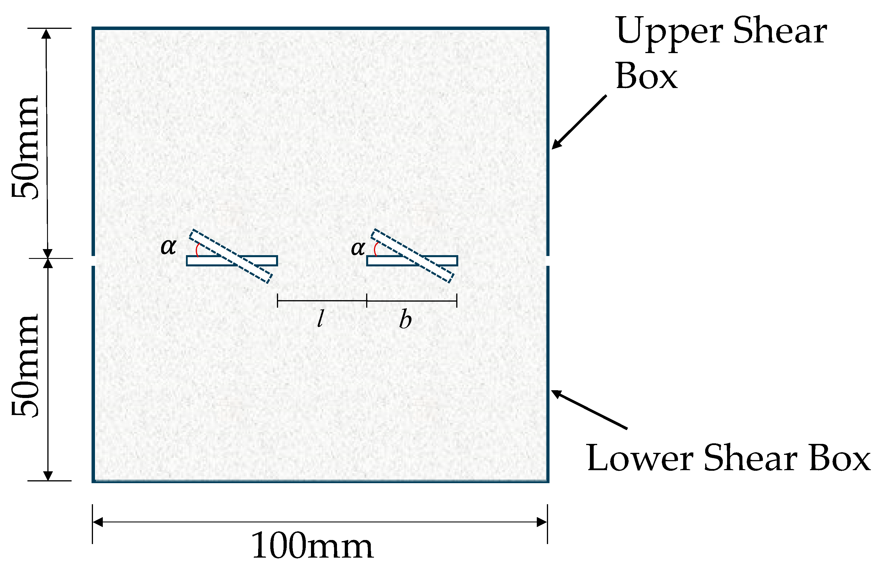
2.1. Laboratory Experiment

Because of the large anisotropy and heterogeneity of natural rock samples, Tai et al. [19] used rock-like materials to simulate rock samples. A mixture of gypsum, water and diatomite was used to prepare the intact samples and jointed blocks, their ratio was 700:280:8. Some fundamental mechanical parameters of rock-like material are shown in Table 1.
In a laboratory experiment, the joints are made by a smooth steel ruler, so that the joint roughness coefficient (JRC) can be considered to be 0. The size of the rock sample is 100 × 100 × 50 mm, the total length of all joints is 40 mm, the rock bridge length is 20 mm, the connection rate is 40%, the joints are coplanar and symmetrically distributed along the center and the rock bridge is divided into three equal-length sections. Figure 1 shows the gypsum samples with the non-persistent joints and geometric parameters of the joints.
The test was performed in a new type of dynamic shear performance test platform for rock discontinuity [20]. The normal load is controlled by force, and the tangential load is controlled by displacement. The normal force applied to the samples was 2.5 kN, and the tangential loading velocity is 0.005 m/s to ensure a quasi-static equilibrium in the direct shear process.

2.2. Numerical Experiment

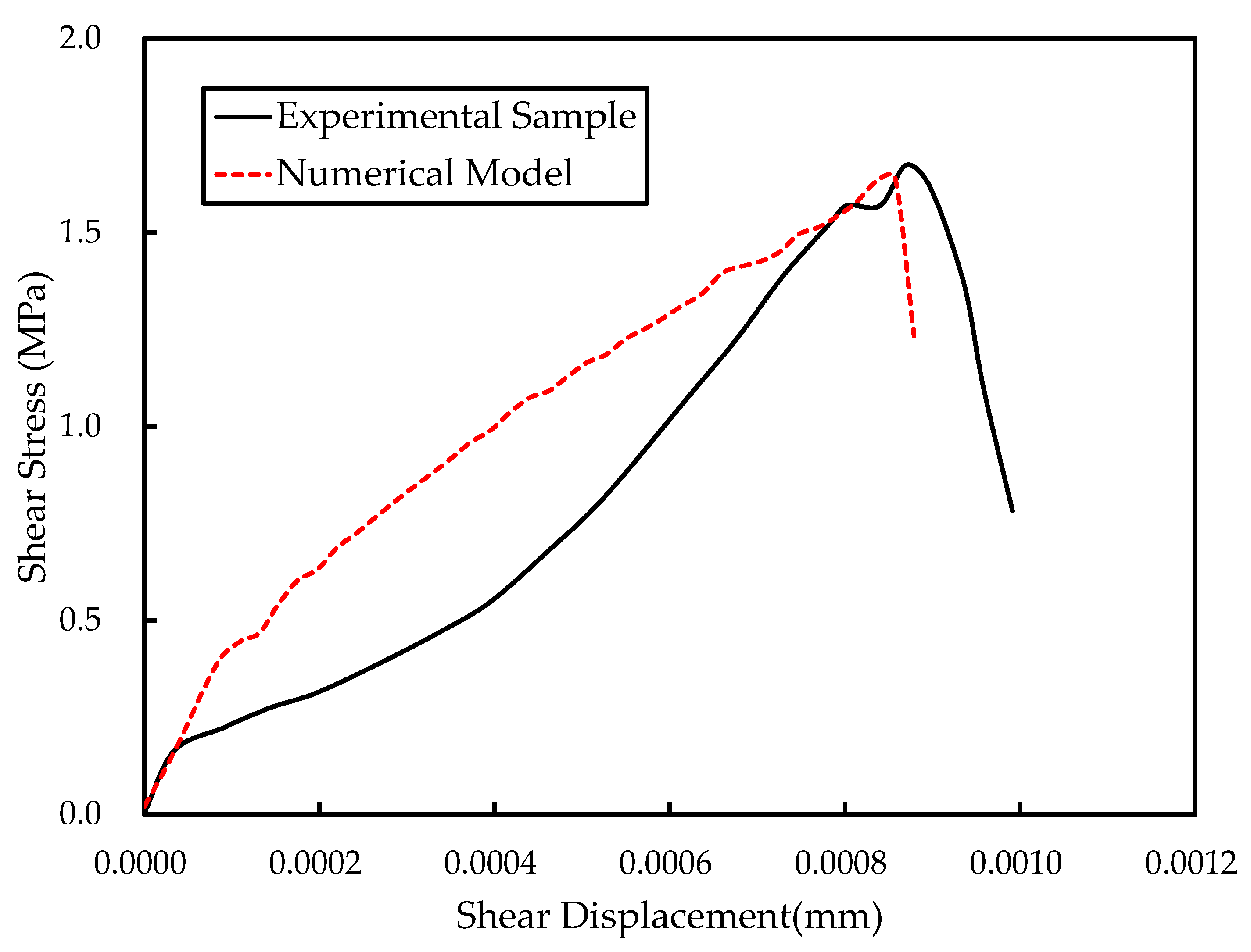
2.2.1. Model Generation and Calibration

To replicate direct shear tests on rock-like samples, a shear box model was devised, featuring eight walls and dimensions of “100 × 100 mm” to align with the laboratory sample sizes, as illustrated in Figure 2. Within this container, a particle mixture with diameters ranging from 0.3 mm to 0.66 mm was generated to fill the space, achieving an initial porosity of 8% for optimal particle connectivity. A total of 12,053 particles were randomly positioned, and appropriate contact models were established between them.
During the numerical experiments, a constant normal force of 2.5 kN was applied to the sample using a numerical servo mechanism. Simultaneously, a shear load was administered by horizontally shifting the upper shear box to the right (as depicted in Figure 1) at a low horizontal velocity (vx = 0.1 m/s). This velocity ensures a quasi-static equilibrium throughout the direct shear process, as highlighted in studies by [19,21,22]. In Particle Flow Code (PFC), the loading velocity is computed via time steps, differing from the physical experiment rates. While these values are not identical, the chosen velocity suffices for quasi-static simulation conditions. Within this framework, the linear parallel bond model simulates intact rocks, and the smooth-joint model is employed for joints.
Particle strength and contact parameters are used to characterize the mechanical characteristics of rock mineral components and cementitious materials in the PFC model. The parameter can be gradually adjusted using a trial-and-error method [23,24], so that the stress–strain curve from numerical experiment approximates the stress–strain curve obtained from the laboratory experiments. When the shear strength and shear modulus of the two are close and the macroscopic failure form is similar, the numerical model constructed can be considered valid. The micromechanical parameters after the final calibration are shown in Table 2 below. The stress–strain curve of the numerical tests at 0° angles of the joints under a normal force 2.5 kN are compared with the results of the laboratory tests as shown in Figure 2, and it can be found that the curve evolution laws of the numerical simulation results and the laboratory test results basically match; however, in contrast to the linear elasticity of the loading stage in numerical calculations, the indoor test curves exhibit concave (hardening) and non-linear characteristics, which is caused by the pores and voids within the specimens. Through the above analysis, it can be seen that the macroscopic mechanical parameters and failure mode of the granular flow model are basically consistent with the indoor laboratory results, so the numerical simulation study can be carried out by this PFC model.

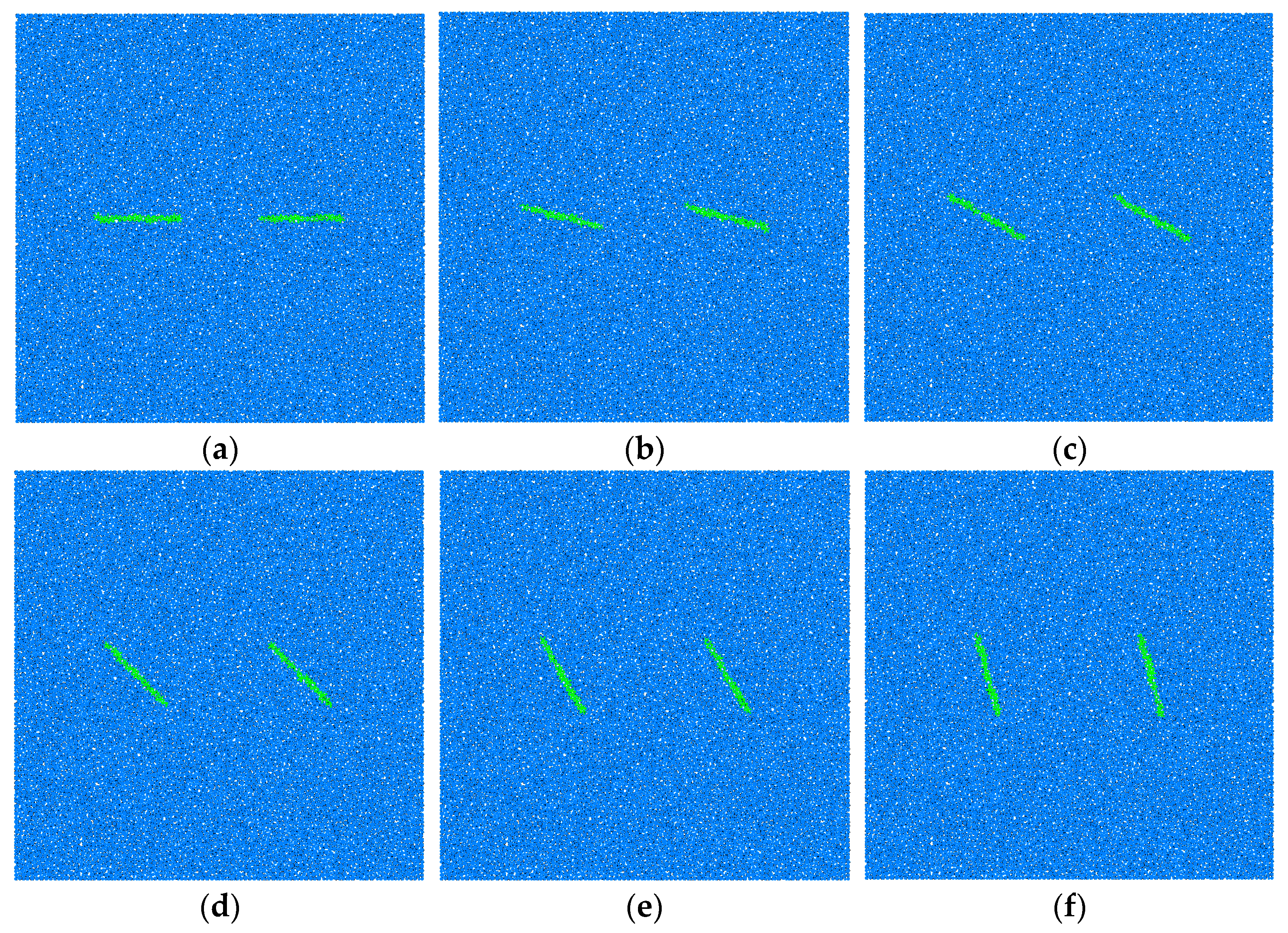
2.2.2. Joint Arrangements for Numerical Analysis

In order to study the effect of the inclination angles of non-persistent joints on shear-induced anisotropy, as shown in Figure 3, where the green section represents the joints and the blue part represents the intact rocks, 12 different models were created in PFC2D 5.0 using the microscopic parameters calibrated in Table 2 and keeping the original model and joint size unchanged. The angle between the joint and the direction of the x-axis is defined as α , and is called the joint inclination (around the midpoint of the joint), as shown in Figure 1. The specimens with 0° of joint inclination were defined as A0°, where “0°” represents the joint’s inclination, so there were A0°, A15°, A30°, A45°, A60°, A75°, A90°, A10°, A120°, A135, A150° and A165° in this study.

3. Results of Numerical Simulation

Using the micromechanical parameters determined above, the PFC model can be used to conduct direct shear tests on rock masses containing different joint inclinations to study the deformation laws and failure mechanisms of the samples from the macroscopic and microscopic levels, including the stress–displacement relationship, failure patterns, the evolution of the fabric and coordination number, the distribution of contact forces and the anisotropic development of the microstructure. We used a personal computer with a CPU model of 12th Gen Intel(R) Core(TM) i7-12700H and 14 cores. It took approximately 50 min to calculate each working condition, and a total of about 600 min in all.

3.1. Deformation and Failure Process

3.1.1. Strength Characteristics of Rock-like Samples Containing Different Joint Inclinations of Non-Persistent Joints

Figure 4 shows the shear strength obtained from numerical simulations under direct shear, Figure 5 shows variations in the peak shear stress with joint inclination, Figure 6 shows variations in the peak displacement with joint inclination; it can be found that joint inclination has a very important influence on the shear mechanical properties of the specimen. The following phenomena can be found from the figures:
(1)
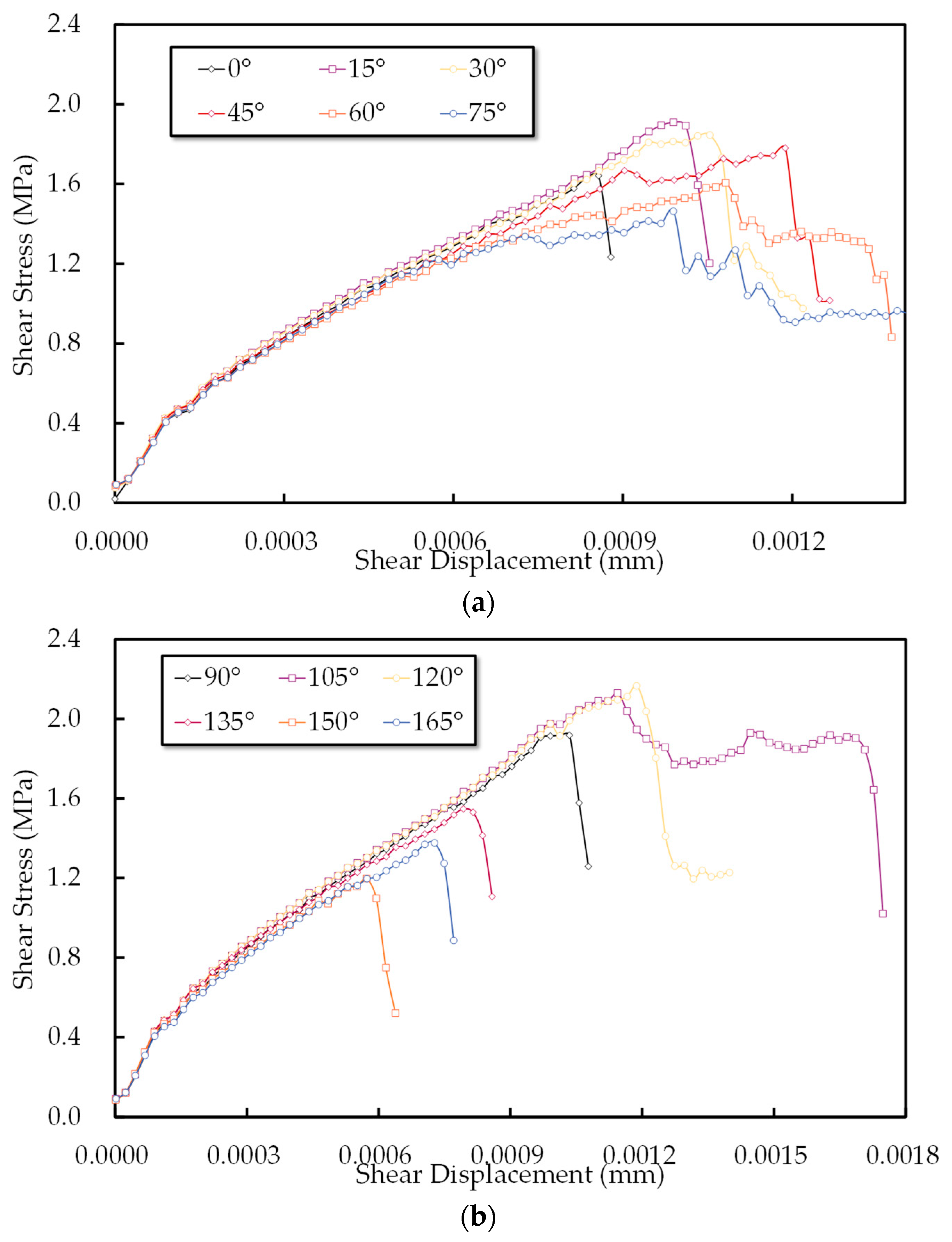
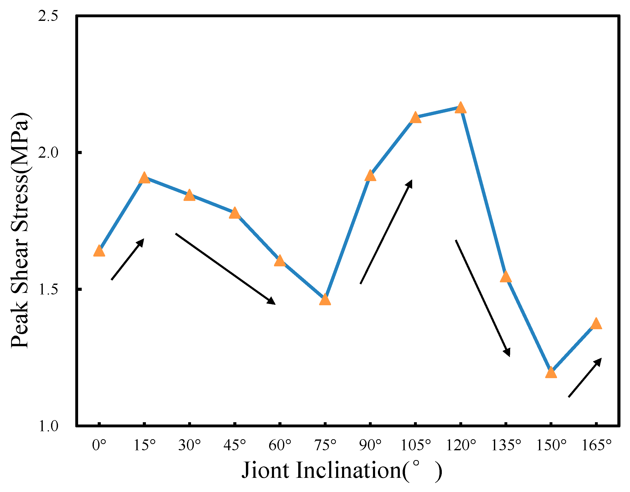
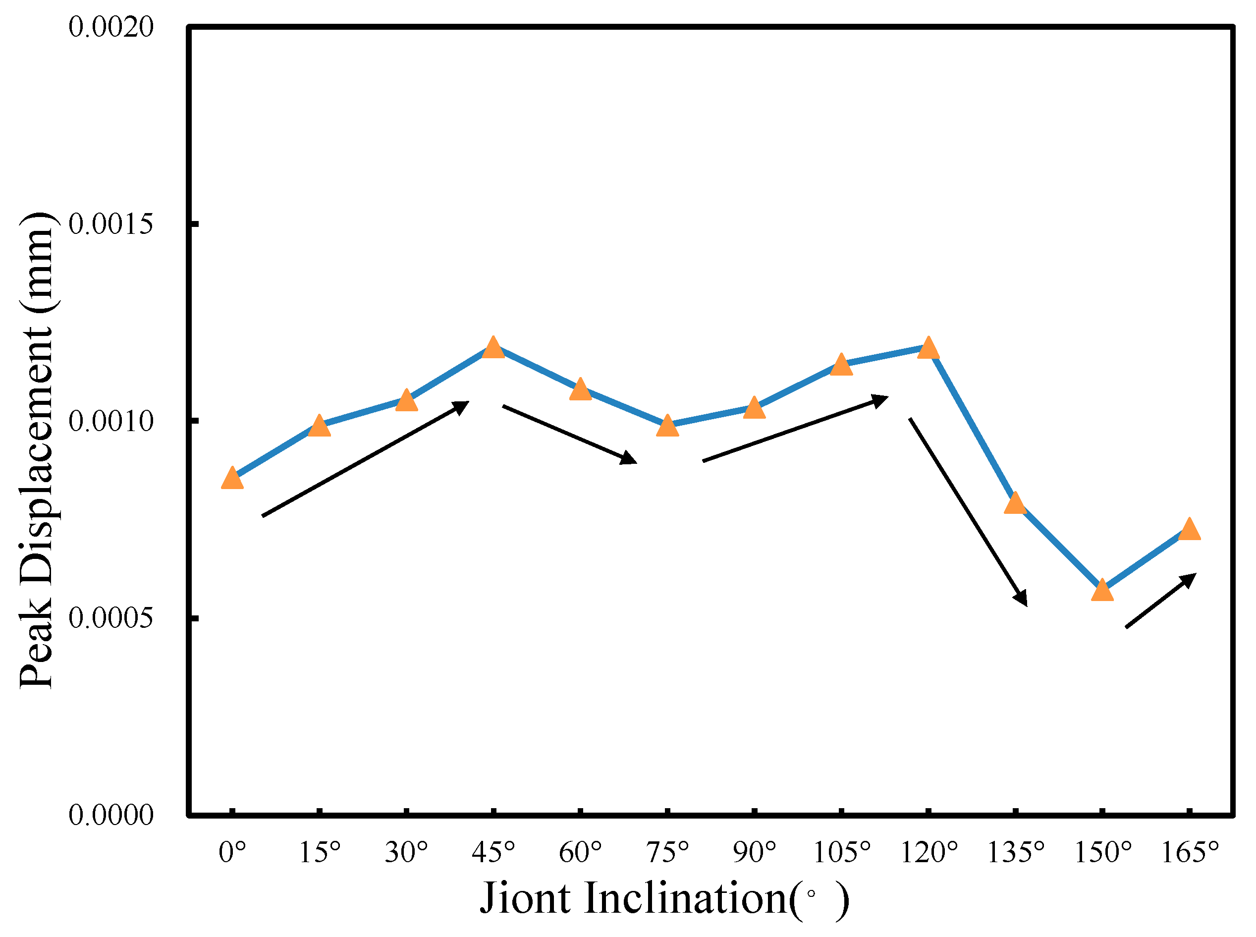
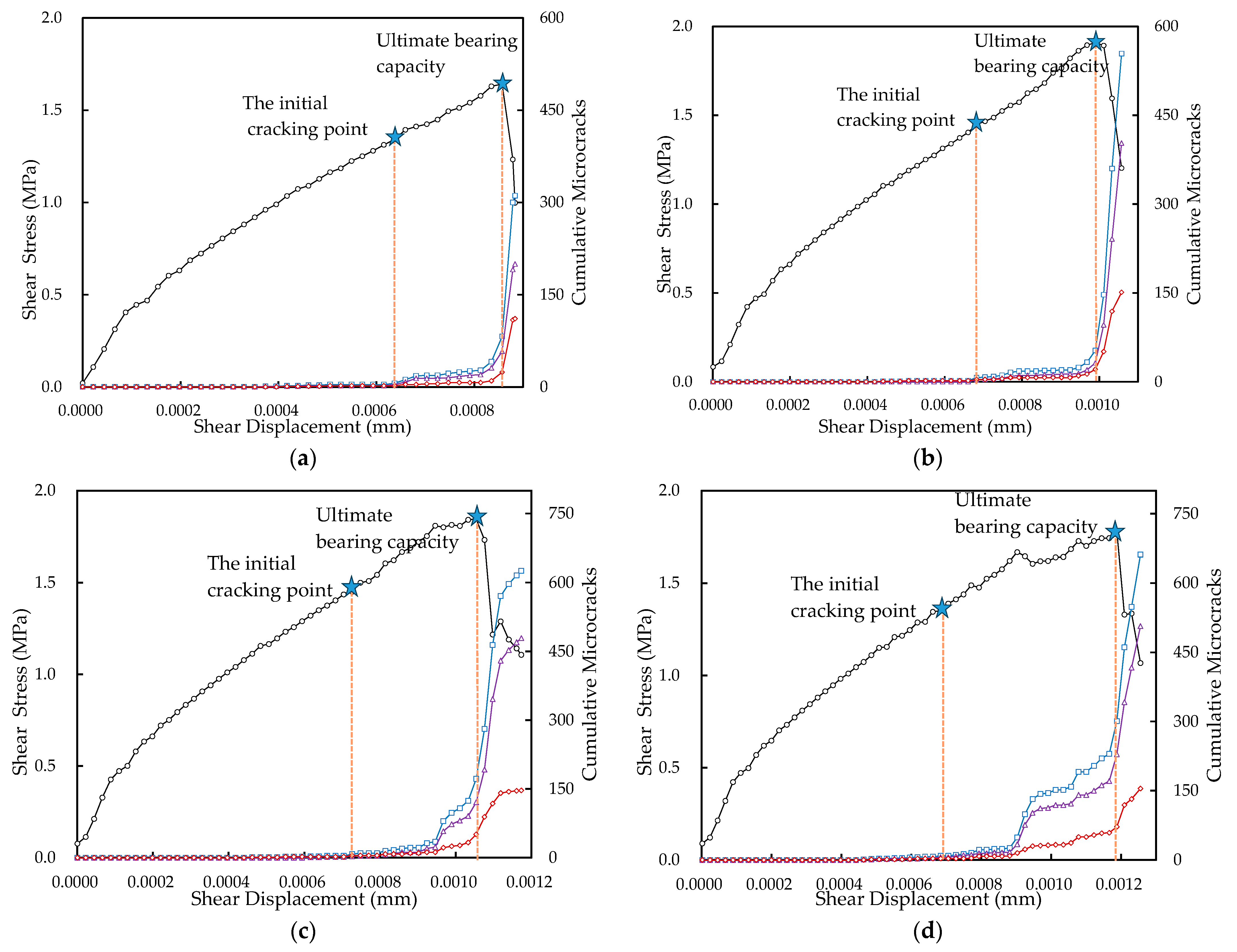
Joint inclination has significant effects on peak shear stress and peak displacement. Under a constant normal load of 2.5 kN, the peak shear stress of 12 specimens with different joint inclination ranges from 1.20 MPa to 2.17 MPa, and the peak displacement ranges from 0.573 mm to 1.189 mm. Both of them show roughly the same trend of variation, showing an increase, then a decrease, then an increase and then a decrease and finally a slight increase. However, the opposite trend was observed in the specimens with joint inclinations of 30° and 45°; this due to the ductile failure of these specimens, which results in a larger peak displacement even with lower peak shear stress;
(2)
Joint inclination plays an important role in the deformability of jointed rock specimens. When the inclination of the joints is the same as the direction of load application, the existence of the joints will make the specimen slide along the joints easily, which makes the specimen’s deformability increase and, at the same time, due to the existence of friction between the joints, the specimen damage tends to be ductile;
(3)
Joint inclination has little effect on the shear bearing capacity and deformation capacity of the specimens in the early loading stage, and it can be noticed from Figure 4 that the stress–displacement curves of the specimens with different joint inclinations in the early loading stage are coincident.
Figure 4. Shear stress–displacement curves of specimens with different joint inclinations. (a) A0–A75°, (b) A90–A165°.
Mathematics 13 00362 g004
Figure 5. Variations in the peak shear stress with joint inclination.
Mathematics 13 00362 g005
Figure 6. Variations in the peak displacement with joint inclination.
Mathematics 13 00362 g006

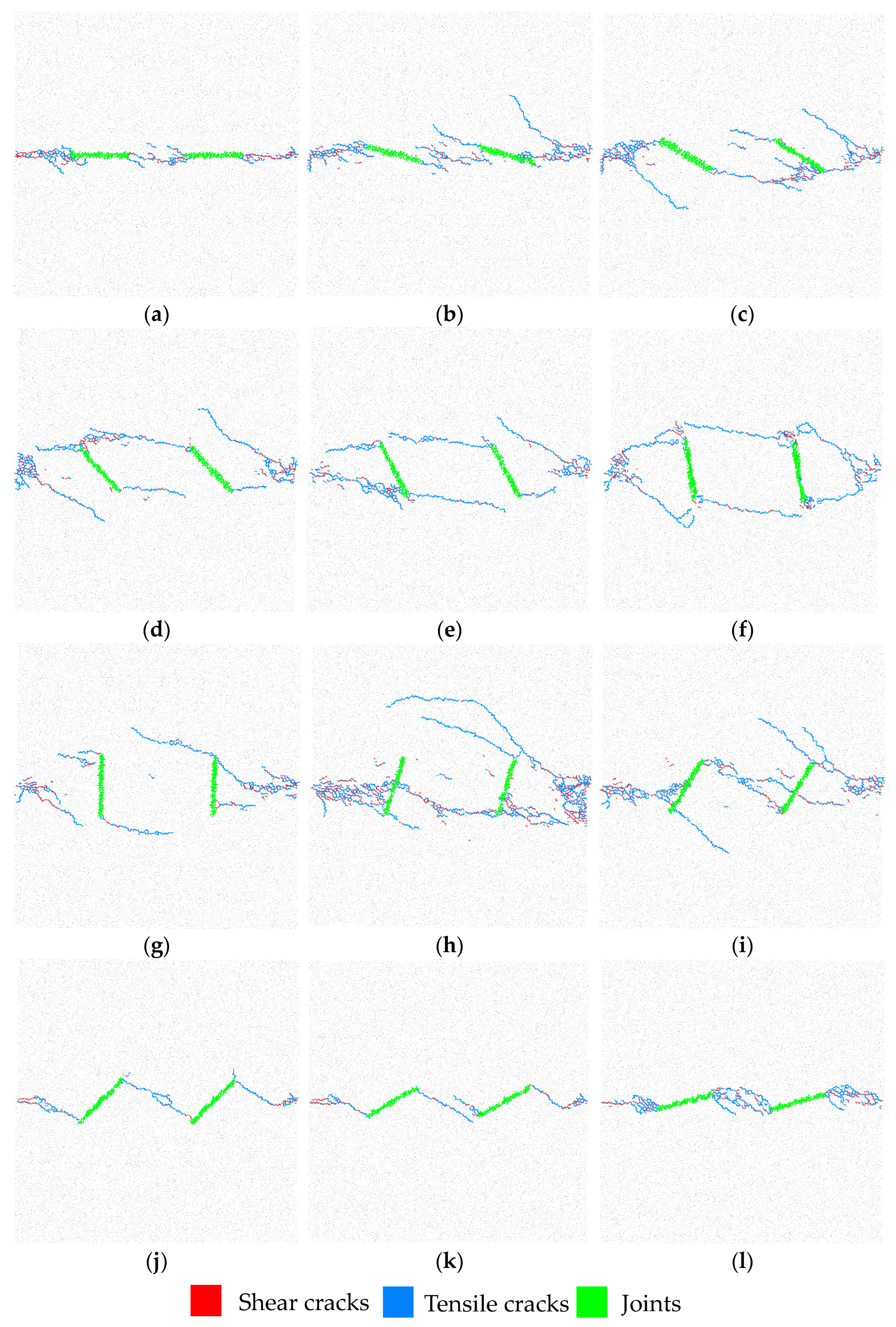
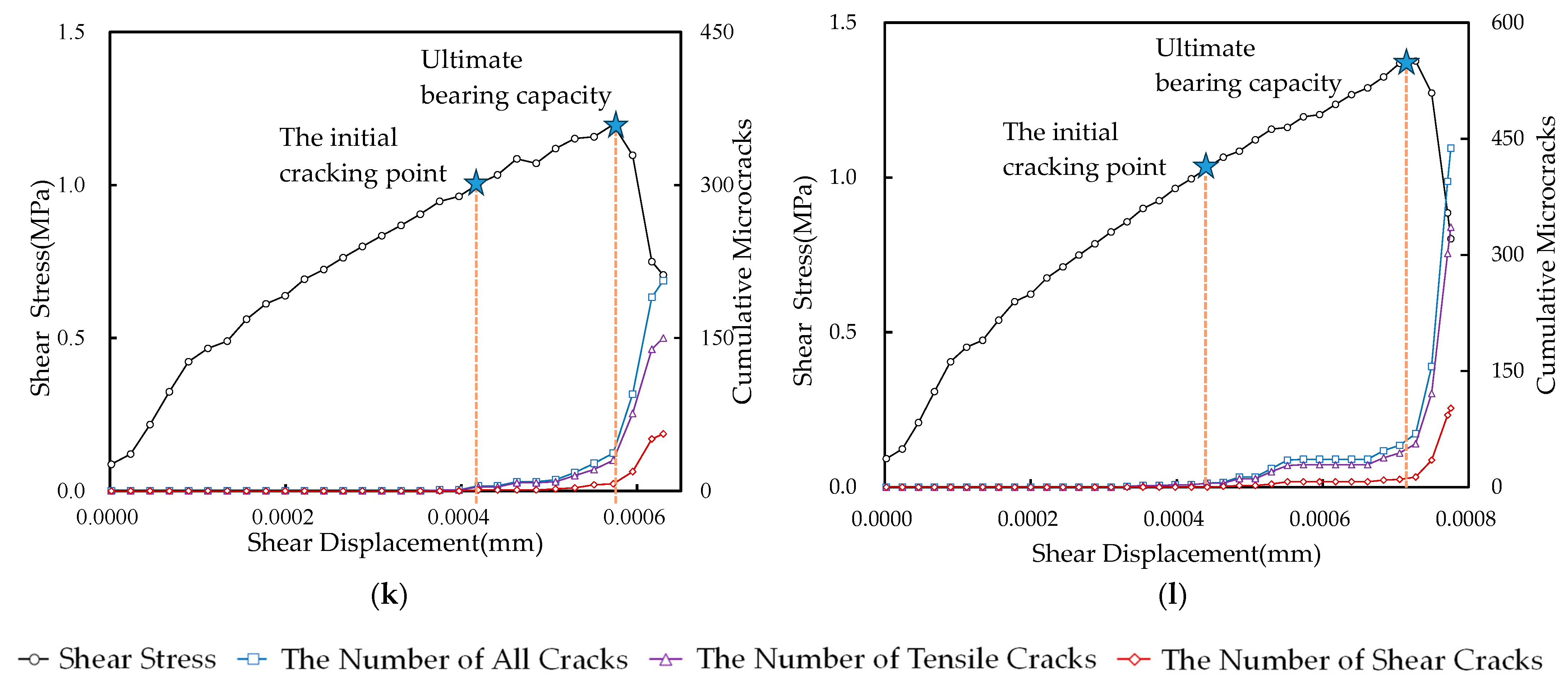
3.1.2. Failure Patterns and Crack Evolution in Specimens

Jointed rocks predominantly exhibit two microcrack modes: tensile and shear cracks. In PFC 5.0, a tensile crack will be identified when the normal contact force between adjacent particles exceeds the set tensile strength of the contact, while a shear crack will be identified when the shear contact force exceeds the critical value based on the Mohr–Coulomb criterion and the particle motion is parallel to the contact plane. As demonstrated in Figure 7, tensile cracks are marked with blue lines, shear cracks with red, and joints with green. It was observed that when the angle between the joint and loading direction is small (e.g., in the 0°, 15°, 135°, 150° and 165° specimens), macroscopic fracture surfaces predominantly propagate along joint surfaces, manifesting a sawtooth failure pattern. As this angle increases, cracks tend to envelop the joints, appearing earlier when the joint dip direction aligns with the shear direction, as discussed by [19,25].
Figure 8 illustrates how crack numbers vary in rock models with different joint inclinations. A sharp rise in crack numbers often accompanies sudden decreases in shear stress, signifying that crack generation and propagation critically influence sample bearing capacity. Microcrack formation is closely tied to material yield, with joint inclination significantly impacting yield properties. In cases where the joint dip direction and shear direction coincide (notably in the 45°, 60° and 75° specimens), failure predominantly occurs through sliding along discontinuities like joints and pre-existing shear-induced cracks. It further reveals a notable distance between the initial cracking and peak shear stress points. These specimens show unique ductile failure traits, including reduced peak strength at high axial strains and a gradual post-peak strength decline. The evolution of cumulative microcracks shifts from rapid increases to a more gradual, step-wise accumulation, especially when the joint dip direction mirrors the shear direction. This change is attributed to shear-induced microcracks encircling joints, as shown in Figure 8d–f. Even under a normal force, these discontinuous surfaces maintain a degree of load-bearing capacity due to friction.

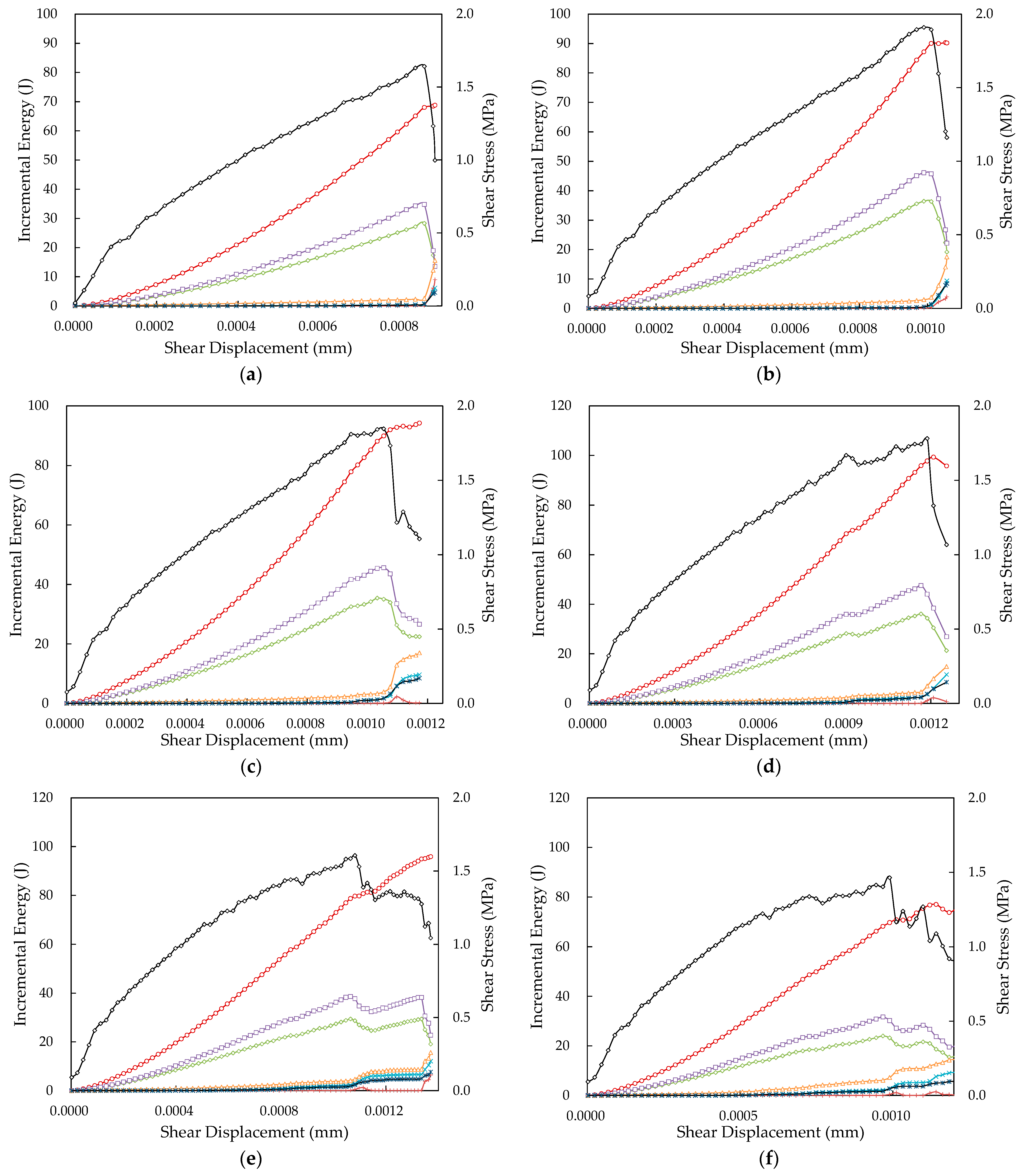
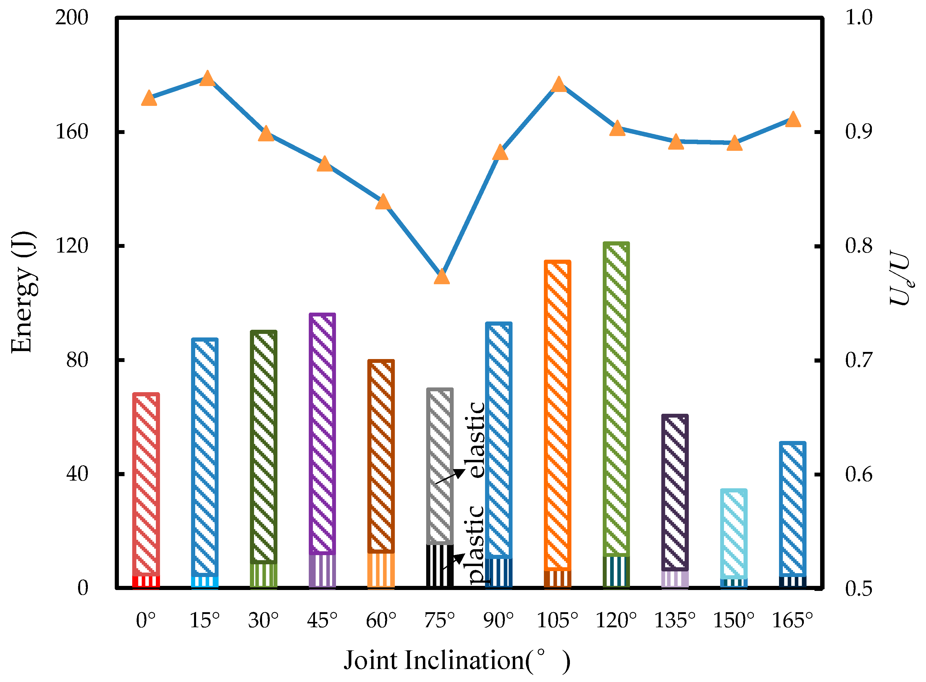
3.1.3. Energy Evolution

Energy is the fundamental cause of rock failure [26], which drives stable specimens into an unstable state. According to the first law of thermodynamics, without considering heat exchange, the following relation is satisfied:
U = U d + U e
where U is the total work of external loads on the specimens, U e is elastic energy dissipation and U d is plastic energy dissipation. Among them, elastic dissipation energy U e includes gravitational potential energy E g , the strain elastic energy stored in particle contact E s , the bond energy stored in particle contact E p b and kinetic energy E k ; plastic energy dissipation U d includes frictional dissipation energy E f , damping dissipation energy E d and fracture energy E f r a c . In this work, gravitational potential energy E g is equal to zero as the gravity acceleration was set to zero [11,27].
The energy input to the system from the wall is expressed by the following equation:
U = 1 2 F w a l l x w a l l
where F w a l l is the force acting on the particle by the wall and x is the displacement occurring in the wall.
Strain elastic energy stored in particle contact E s can be calculated by:
E s = 1 2 N c F i n 2 k ¯ n + F i s 2 k ¯ s
where F i n and F i s are normal and horizontal loads and k ¯ n and k ¯ s are the normal and shear stiffnesses of the contacts.
Bond energy stored in particle contact E p b is defined as:
E p b = 1 2 N p b F ¯ i n 2 A k n + F ¯ i s 2 A k s + M ¯ i n 2 J k s + M ¯ i s 2 I k s
where F ¯ i n and F ¯ i s are the normal and tangential forces of the parallel bond, respectively; k n and k s are the normal and shear stiffnesses of the parallel bond; M ¯ i n and M ¯ i s are the normal and tangential components of the torque, respectively; A is the area of inertia of the cross-section of the parallel bond; and J and I are the polar moment and the moment of inertia of the parallel bond cross-section, respectively.
Frictional dissipation energy E f is the energy consumed by the friction between particles, with
E f = N c F s U i s s l i p
where F s is the average shear force and U i s s l i p is the increment of slip displacement.
Kinetic energy E k is the energy consumed by particle motion, with
E k = 1 2 N p m i v i 2
where m i is the mass of a particle with the ID i and v i is the velocity of a particle with the ID i.
Fracture energy E f r a c is equal to the strain elastic energy stored in particle contact E s at the onset of failure.
Figure 9 illustrates the energy distribution in specimens under direct shear loading, varying with joint inclination. Initially, boundary energy primarily converts into strain elastic energy and bond energy. The emergence of microcracks signals the start of inelastic dissipation, altering the energy dynamics. The absorbed energy in rock specimens is no longer confined to elastic strain energy and bond energy but also includes plastic energy dissipation due to extensive frictional movement along existing joint surfaces and microcracks induced by shear loading.
Microcracks themselves dissipate only a minor fraction of the external work, primarily facilitating additional degrees of freedom for frictional sliding across discontinuities and between particles, thus influencing the microstructure of solids. Notably, when the joint dip direction aligns with the shear direction, particularly in specimens with joint inclinations of 45°, 60° and 75°, sliding along discontinuities becomes the primary failure mechanism. This increases the proportion of frictional energy consumption in the total energy budget, leading to specimens exhibiting ductile failure characteristics. Conversely, when the joint dip direction opposes the shear direction, as seen in specimens with joint inclinations of 135°, 150° and 165°, microcracks tend to propagate from the joint ends in a direction similar to the loading. This causes the particles on either side of the microcracks to progressively detach during shear, impeding the dissipation of input energy through plastic mechanisms like friction. As a result, these specimens demonstrate a lower energy-bearing capacity and exhibit brittle failure characteristics.
Figure 10 presents the relationship between the proportion of elastic energy to the total input energy at peak conditions, alongside the values of elastic and plastic energy for various samples. An observed trend is the correlation between the proportion of elastic energy and peak strength. This correlation predominantly arises due to changes in the consumption of friction energy. Generally, a higher peak stress correlates with a greater capacity of the specimens to store elastic energy, consequently increasing the proportion of elastic energy. Additionally, this proportion is influenced by the failure mode of the specimens. In cases where specimens demonstrate ductile failure, increased energy dissipation through friction results in a reduced proportion of elastic energy. Conversely, specimens with larger joint inclinations tend to have a higher proportion of elastic energy, which can be attributed to their failure mode.

3.2. Micromechanism and Macroresponse

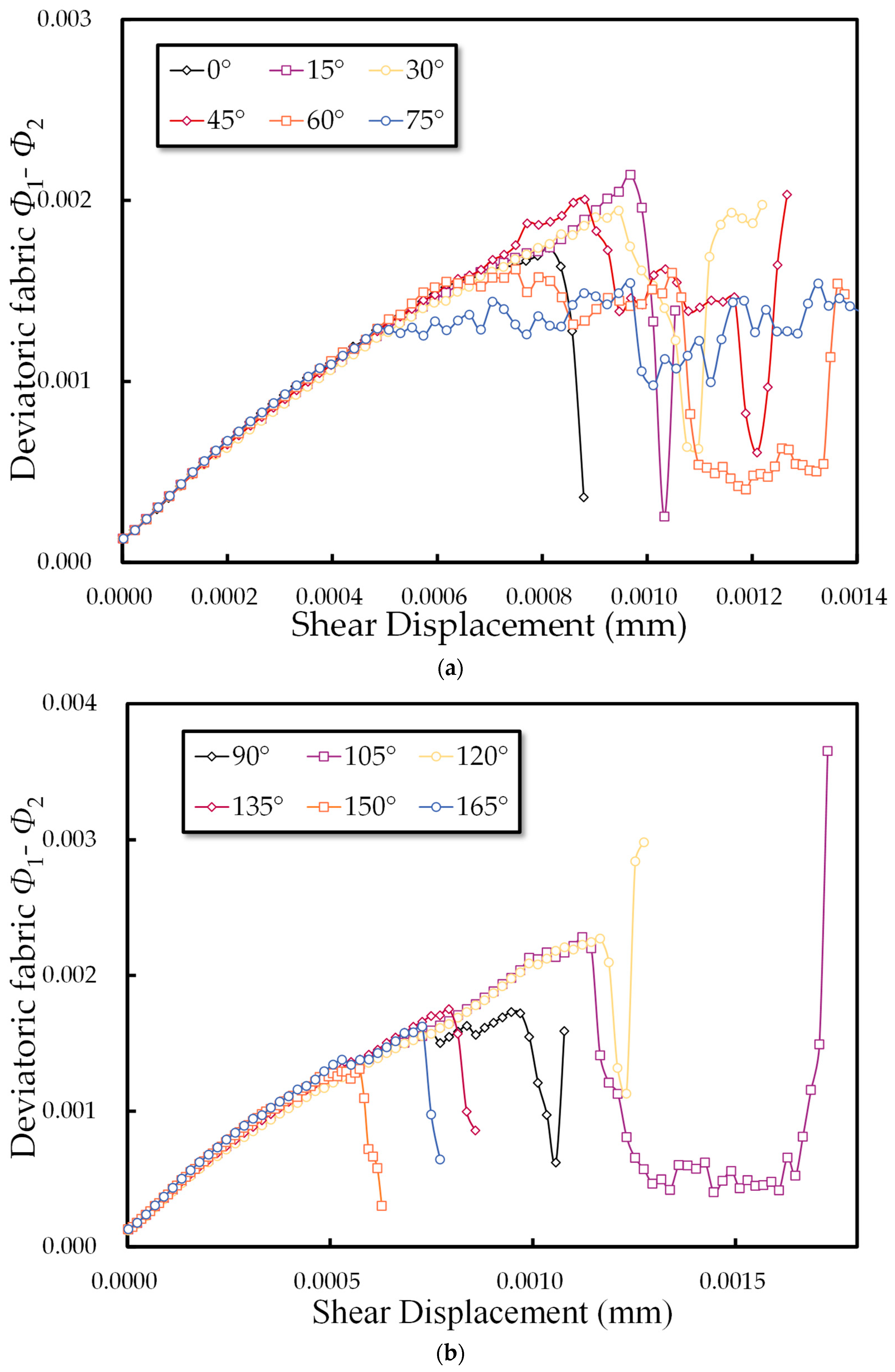
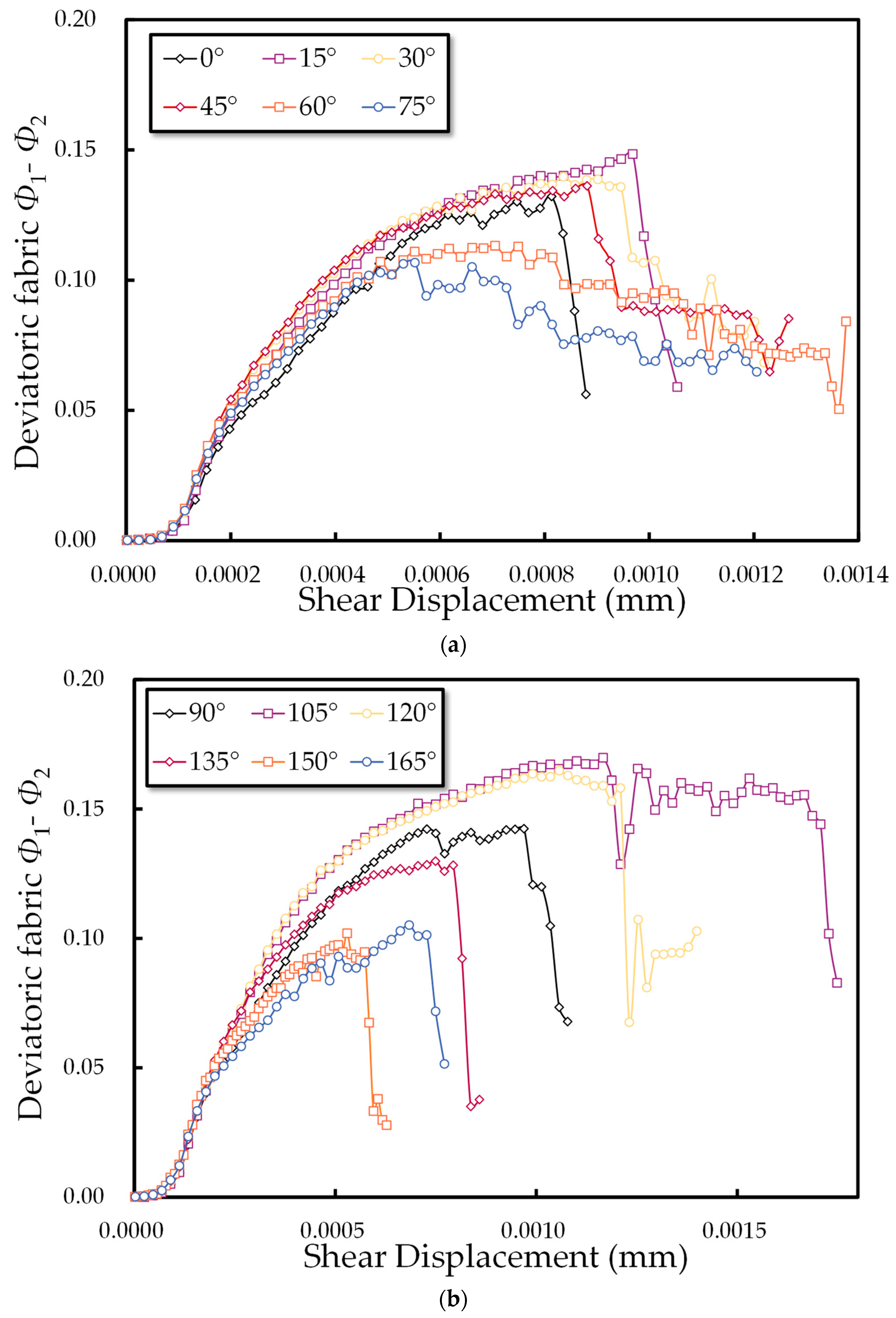
3.2.1. Evolution of Fabric

In the study of the microstructure of granular materials, the fabric tensor can be used to observe the changes in microstructure through the average direction vector and the amplitude of the vector. Satake pointed out that for disks or circular particles [28], the fabric tensor can be defined by using a second-order tensor, the tensor ( Φ i j ) is given as:
Φ i j = 1   N c N c n i n j
where Nc is the total number of contacts, n is the unit normal vector of contact with i and j = 1, 2 for two-dimensional (2D) analyses. The contact normal is defined as vectors that are perpendicular to the plane, defining the contact between two particles. The summation and averaging are taken over all Nc contacts in the contact network.
The eigenvalues of the fabric tensor provide the main textures Φ 1 and Φ 2 , which can be used to describe the degree of anisotropy. The degree of anisotropy can be characterized by [29]:
Φ 1 Φ 2 = 2 Φ 11 Φ 22 2 2 + Φ 21 2
This study analyzed three sets of contact normals: (i) considering all engaged contacts, (ii) contacts that only transmit compressive force and (iii) contacts that only transmit tensile force. The corresponding variation in the deviatoric fabric of the contact normal with displacement is shown in Figure 11, Figure 12 and Figure 13.
The deviatoric fabric’s magnitude and evolution differ across contact types. When considering all contacts (refer to Figure 11), the initial phase of loading shows a nearly linear increase in deviatoric fabric, transitioning to a nonlinear deflection upon microcrack formation in the specimen. At peak stress, there is a rapid decrease in deviatoric fabric. Notably, specimens with higher peak stresses align with larger peak deviatoric fabric values, as indicated by a comparison with Figure 5. In ductile damage specimens, the deviatoric fabric exhibits a gradual increase before the peak and maintains a significant residual post peak. For some specimens, there is an initial rapid decrease in deviatoric fabric after peak damage, followed by a notable increase, attributed to the loss and subsequent formation of new contacts at macrocrack sites as loading progresses.
Figure 12 highlights the deviatoric fabric variation in contacts transmitting only compressive force with shear displacement. It reveals that joint inclination significantly influences the evolution of deviatoric fabric in these contact groups. Specifically, certain joint inclinations can suppress contact strength and microstructural evolution, diminishing the specimen’s load-bearing capacity. Post peak, a rapid decrease in deviatoric fabric is observed in some specimens, correlating with the breakdown or collapse of the compression contact network characteristic of brittle failure. Conversely, a slow decrease following microcrack emergence indicates a gradual compression network collapse, aligning with ductile failure.
Figure 13 details the deviatoric fabric changes in contacts transmitting only tensile force with shear displacement. The initial evolution is varied, with some specimens exhibiting a rapid increase and decrease. This pattern is due to the absence of tensile stress during initial isotropic compaction and its emergence with shear load application. A stable increase follows, then a decrease after specimen damage. Notably, the deviatoric fabric in tensile contacts is generally much higher than in compressive contacts.

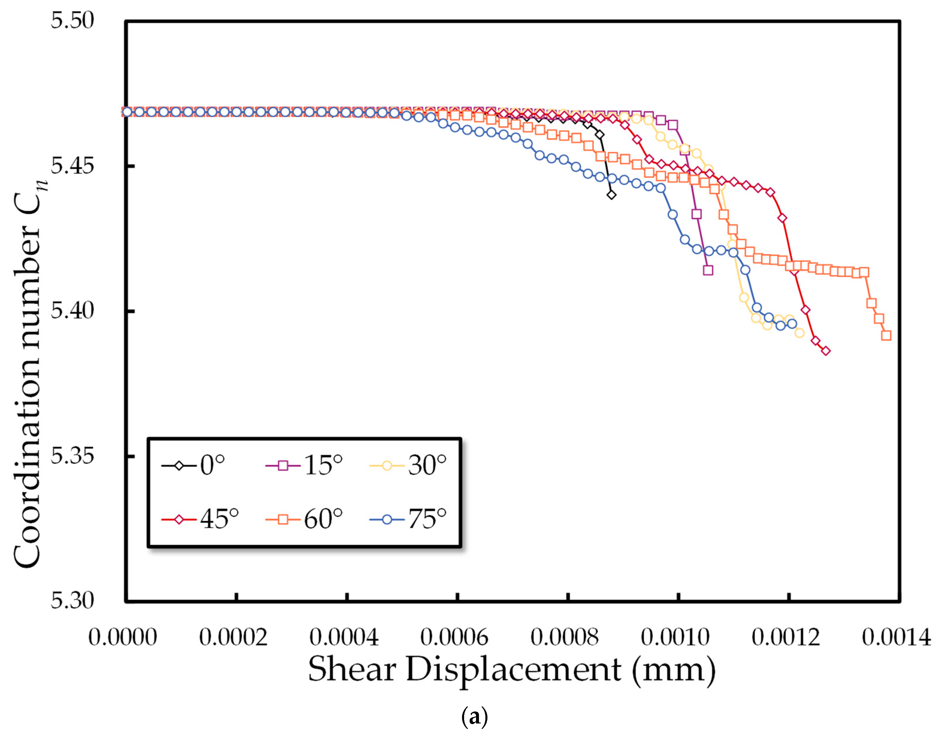
3.2.2. Evolution of Coordination Number

In the realm of discrete element numerical simulations, researchers have introduced numerous quantitative metrics to characterize the micro-level properties of granular materials. A key indicator among these is the coordination number. This number represents the average count of inter-particle contacts within a particle assembly, as defined by [30]:
C n = 2 N c N p
where N p is the number of particles and N c is the number of their contacts.
Figure 14 illustrates the displacement-related changes in the coordination number. Initially, the coordination number stays constant for a period, signifying unbroken contacts within the specimens. A sudden decline at a certain point indicates the breakdown of bonding contacts in most rock block specimens. In contrast, for specimens where the dip direction of joints aligns with the shear direction (notably those with joint inclinations of 45°, 60° and 75°), the coordination number gradually decreases after the emergence of microcracks and continues until specimen destruction. This pattern elucidates the micro-level mechanisms underlying ductile failure. The rate at which the coordination number changes is intimately linked to the breaking patterns of the particle aggregates.

3.2.3. Introduction to Microstructure Anisotropy

In assessing a particle system’s anisotropy, two distinct categories are recognized: geometric anisotropy and mechanical anisotropy. Geometric anisotropy refers to the particular alignment of contact planes at the local level, which contributes to the overall anisotropic behavior observed. Mechanical anisotropy, conversely, arises primarily due to external forces and is influenced by the contact forces relative to the orientations of these contact planes. In a collection of circular particles, the concept of geometrical anisotropy can be quantified by examining the distribution of the contact normal vectors.
According to the point contact assumption, the contact normal can be defined as the unit vector normal of the particle surface at the contact point; each contact point is associated with two contact normals, represented by the unit normal vectors n and n ; the probability density of the contact point normals can be approximated by the even function E c ( n ) , which is symmetric with direction n , i.e., E c n = E c n . Due to E c n is a probability density distribution, so must satisfy [31,32]:
Ω E c ( n ) d Ω = 1 and   E c ( n ) 0
Therefore, the fabric tensor of contact normals can be defined as:
Φ i j = Θ E c n n i n j d Θ = 1   N c N c n i n j
Using the polynomial of the unit direction vector n and the indefinite coefficient, the approximate form of n-th rank is as follows [33]:
E c n = E 0 a i 1 i 2 i n c n i 1 n i 2 n i n
where E 0 = 1 / n i d n i . In the two-dimensional case, E 0 = 1 / 2 π . The rank of the approximation refers to the highest rank of the power terms in the polynomial expansion. For symmetric distributions, the rank of approximation in Equation (19) should only be even numbers, and the direction tensor a i 1 i 2 i n c is a symmetric tensor, i.e., a i 1 i 2 i n c = a i 1 i 2 i n c over the subscripts designates the symmetrization of the indices. a i 1 i 2 i n c is referred to as the direction tensor for contact normal density. In the two-dimensional case, considering accuracy and computational efficiency, only second-order Fourier extensions can be taken [34,35]:
E c n = 1 2 π 1 + a i j c n i n j
Bringing Equation (19) into Equation (18) and integrating, we obtain:
Φ i j = 1 2 δ i j + a i j c 4
Among these terms, δ i j is the Kronecker delta; the second-order tensor a i j c is deviatoric and symmetric, indicating fabric anisotropy. In short, acij can be represented by the deviation tensor Φ i j given by Equation (22):
a i j c = 4 Φ i j
Considering that there are two opposite contact normals at each physical contact point, and that they are related to two adjacent particles, the parameter E c n which characterizes the distribution of the contact normal direction can be determined from discrete data.
In the two-dimensional case, any direction n i can be expressed by its angle θ, i.e., n i , n j = cos θ , sin θ to be expressed by bringing in Equation (13) to obtain
E c n = 1 2 π 1 + a 11 c a 22 c 2 cos 2 θ + a 12 c + a 21 c 2 sin 2 θ = 1 2 π 1 + a c cos 2 θ θ c
In which a c = a 11 c a 22 c 2 + a 12 c + a 21 c 2 / 2 and tan 2 θ c = a 11 c a 22 c / a 12 c + a 21 c . a c characterizes the anisotropic degree, and θ c gives the major principal direction. The above equation is actually a truncated Fourier series with zero- and second-order terms.
Similarly to the probability density function of the contact direction, mechanical anisotropy can be split into normal force anisotropy (caused by normal contact forces) and tangential force anisotropy (induced by tangential contact forces), which are, respectively, defined as follows [36]:
χ i j n = 1   N c c N c f n n i n j 1 + a k l c n k n l = 1 2 π Θ f n ¯ Θ n i n j d Θ
f ¯ i n Θ = F i n n i = f ¯ 0 1 + a k l n n k n l n i
and
χ i j t = 1   N c c N c f t t i n j 1 + a k l c n k n l = 1 2 π Θ f t ¯ Θ n i n j d Θ
f ¯ i n Θ = F i n n i = f ¯ 0 1 + a k l n n k n l n i
where
a i j n = 4 χ i j n f ¯ 0 , a i j t = 4 χ i j t f ¯ 0
Bringing t i , t j = sin θ , cos θ and n i , n j = cos θ , sin θ into Equations (18) and (20) we can obtain:
f ¯ n Θ = f ¯ 0 1 + a 11 n a 22 n 2 cos 2 θ + a 12 n + a 21 n 2 sin 2 θ = f ¯ 0 1 + a n cos 2 θ θ n
f ¯ t Θ = f ¯ 0 a 11 t a 22 t 2 sin 2 θ + a 12 t + a 21 t 2 cos 2 θ = f ¯ 0 a t sin 2 θ θ t
In which the directional distributions of the force components are characterized by the anisotropic degree, a n and a t , and the major principal directions, θ n and θ t . It is easy to determine their values as:
a n = a 11 n a 22 n 2 + a 12 n + a 21 n 2 2
a t = a 11 t a 22 t 2 + a 12 t + a 21 t 2 2
t a n 2 θ n = a 12 n + a 21 n a 11 n a 22 n
t a n 2 θ t = a 12 t + a 21 t a 11 t a 22 t

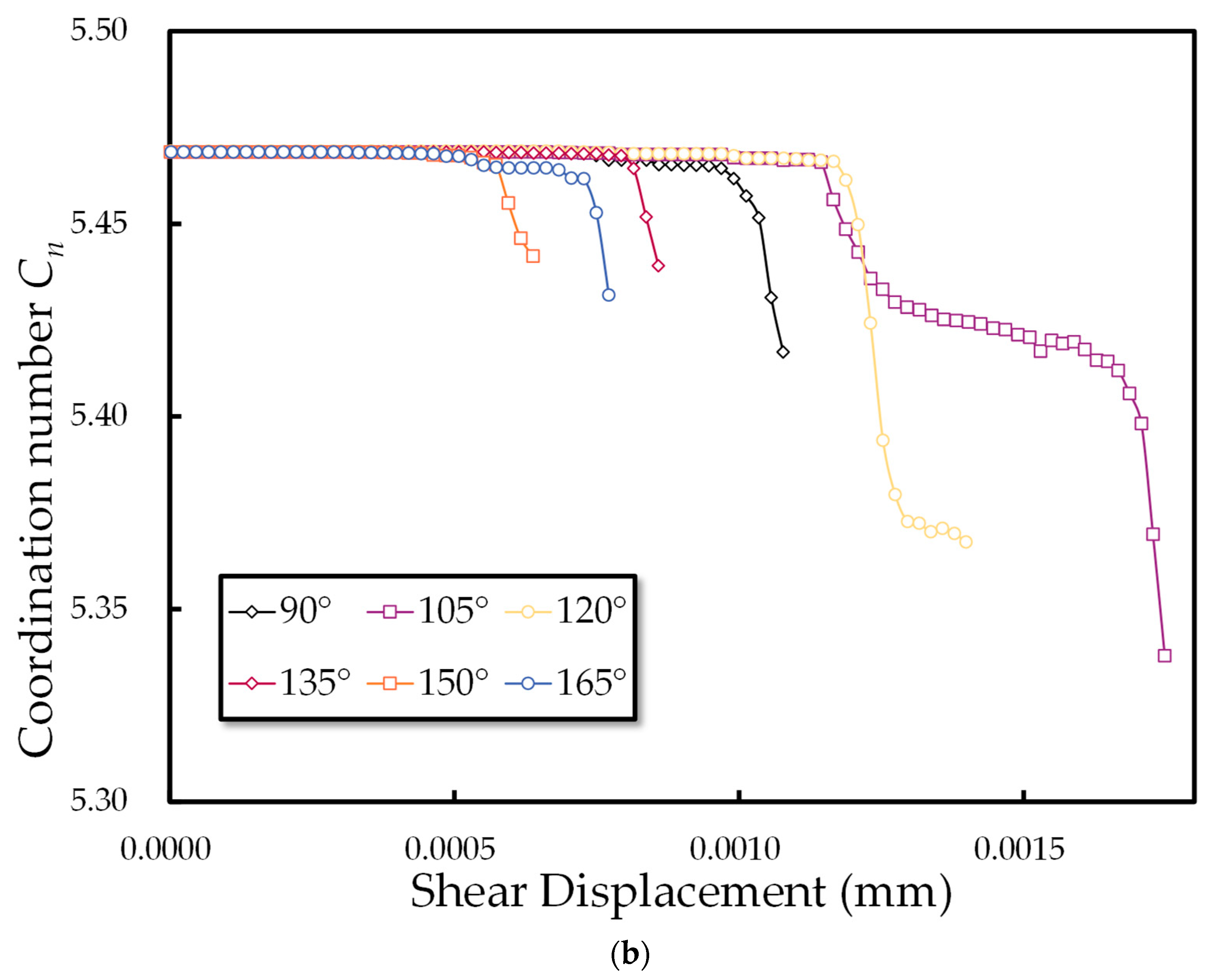
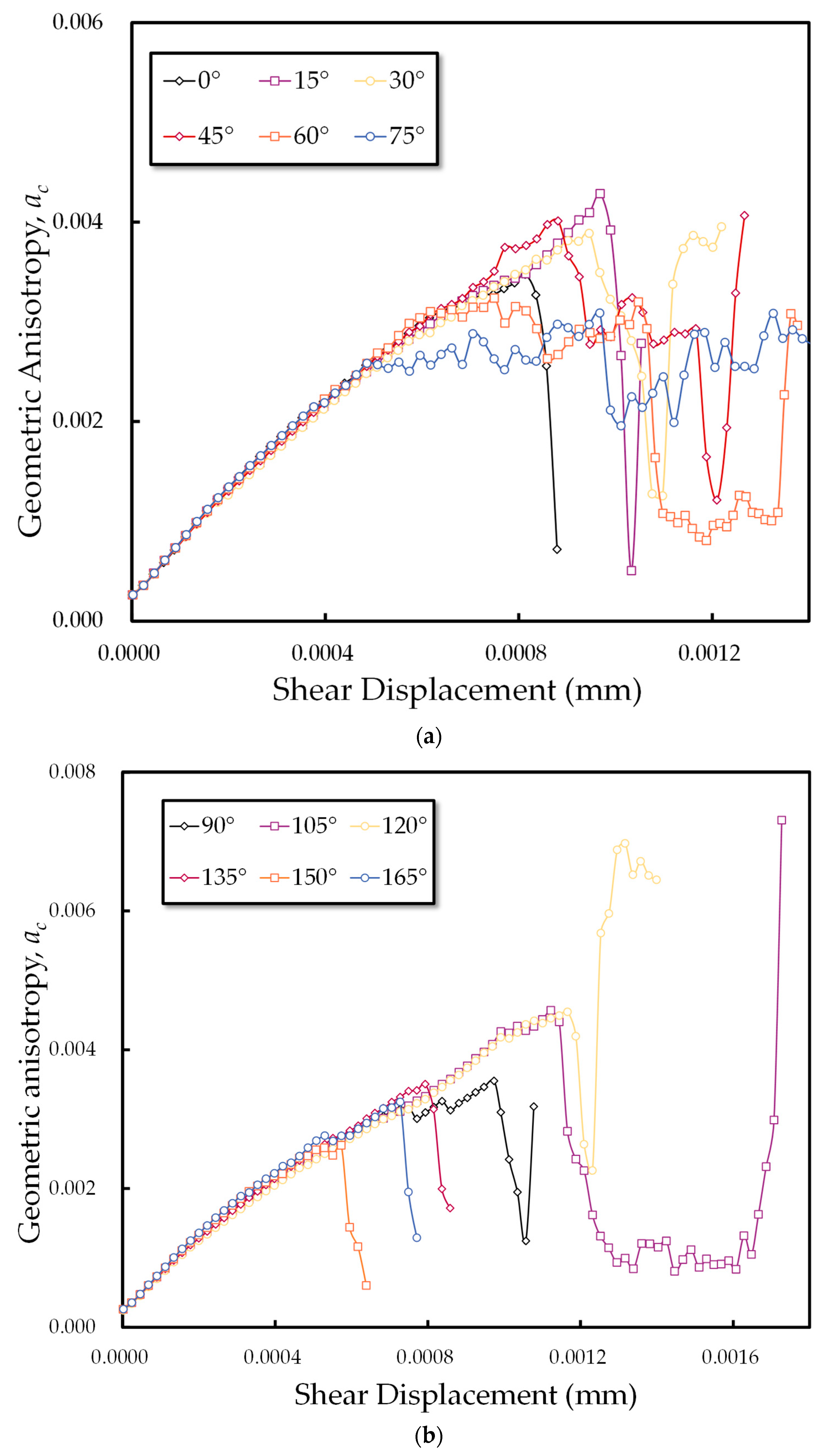
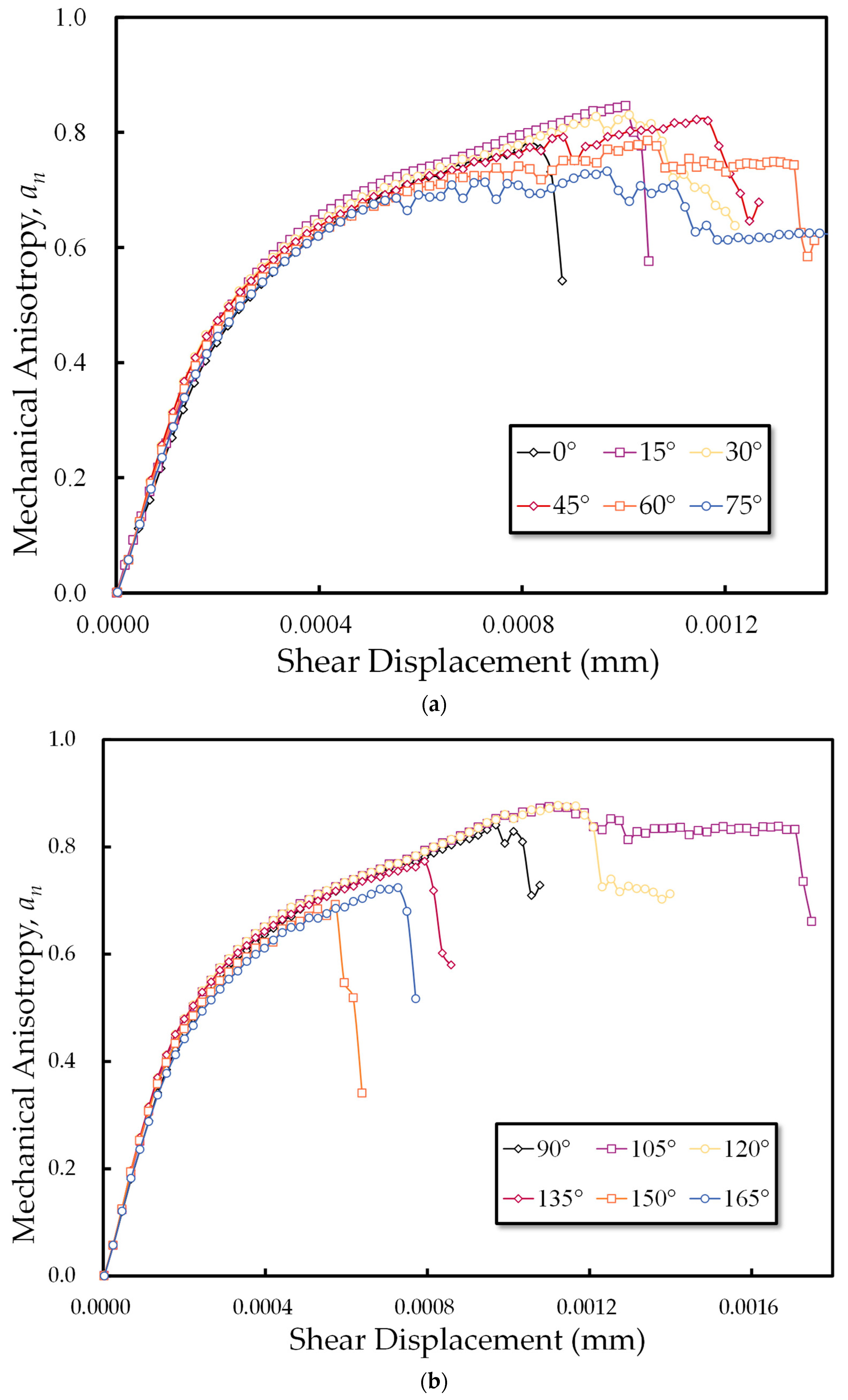
3.2.4. The Evolution of the Anisotropy of Microstructure During the Numerical Experiment

The evolution of the anisotropy coefficients a c , a n and a t of different rock specimens during the numerical experiment is shown in Figure 15, Figure 16 and Figure 17.
Although the deviation fabric is equal to a c / 2 , the evolution trend of the normal anisotropy ( a c ) of the contacts is the same as that of the deviation fabric (Figure 6). Therefore, there is no need to further discuss the evolution of contact normal to anisotropy in this article.
The coefficients a n and a t exhibit a broadly similar trend throughout the loading process. Initially, both coefficients rise, mirroring the pattern observed in the shear stress–displacement curve (Figure 4). Early in the loading phase, the evolution of a n and a t across different specimens is nearly identical, with their respective curves closely aligned. However, following the emergence of microcracks, these curves start to diverge. Specimens with higher peak shear strengths typically demonstrate larger peak values for both a n and a t . After the specimens reach their peak shear stress, these coefficients decline rapidly, reflecting the creation and breakdown of microstructures. The decline of a n and a t signifies the integration of new microcracks with existing ones, forming larger cracks.
Notably, all specimens exhibit a swift increase in mechanical anisotropy, though the growth rate after microcrack formation varies with joint inclination. For specimens where the joint dip direction aligns with the shear direction (notably at the 45°, 60° and 75° inclinations), joint effects dampen particle dynamics and the friction from microcracks decelerates the growth of a n and a t before the peak, with a more gradual decline post peak, indicative of ductile failure characteristics. Conversely, in specimens with opposing joint and shear directions (especially at the 135°, 150° and 165° inclinations), fewer microcracks form pre peak, leading to a near-constant a n and a t value before failure. At peak stress, microcracks accumulate rapidly. Due to particle separation at microcrack extremities under shear stress, frictional forces fail to adequately dissipate input energy, leading to particle contact loss, a steep drop in a n and a t values and a reduction in load-bearing capacity, manifesting as brittle failure.

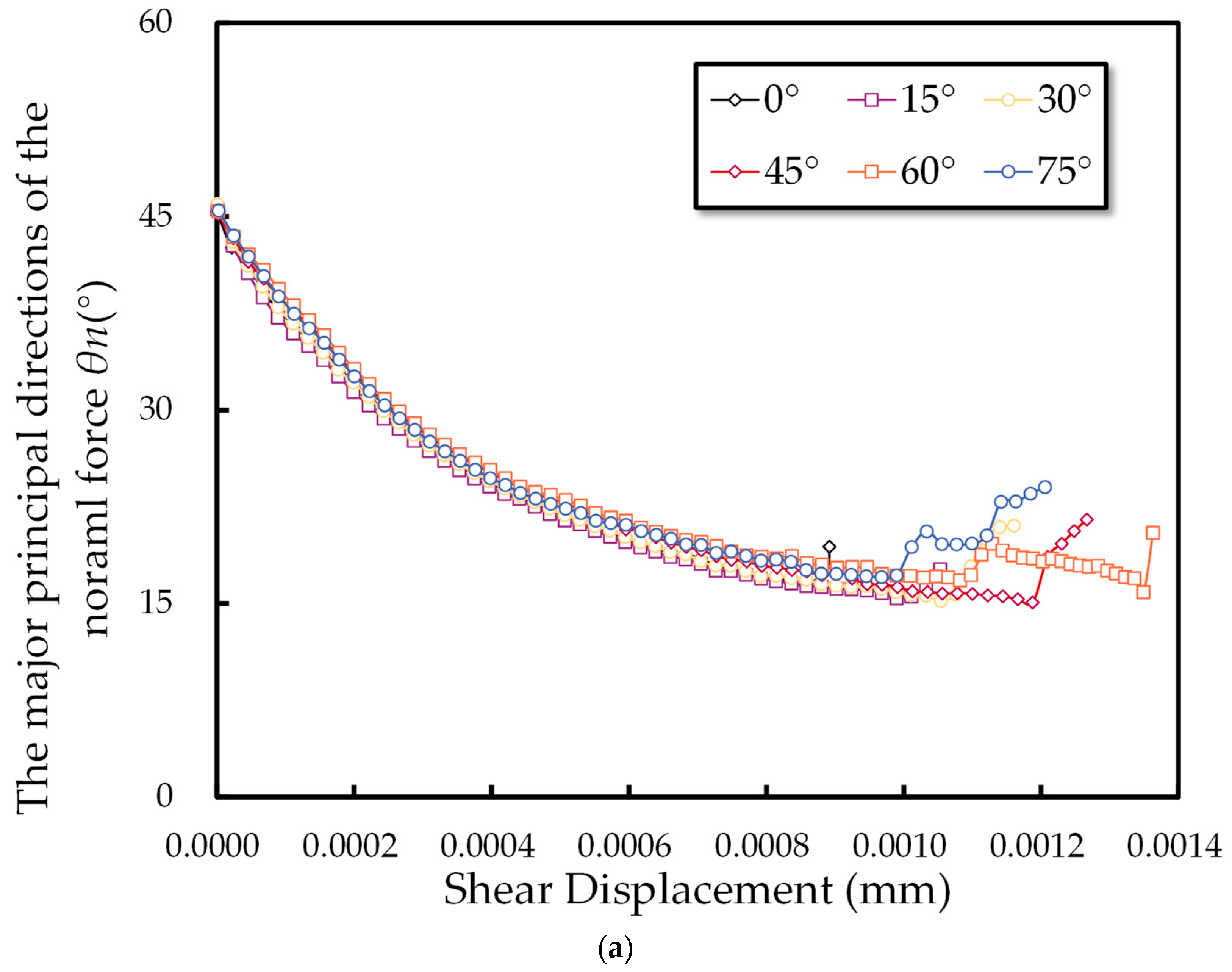
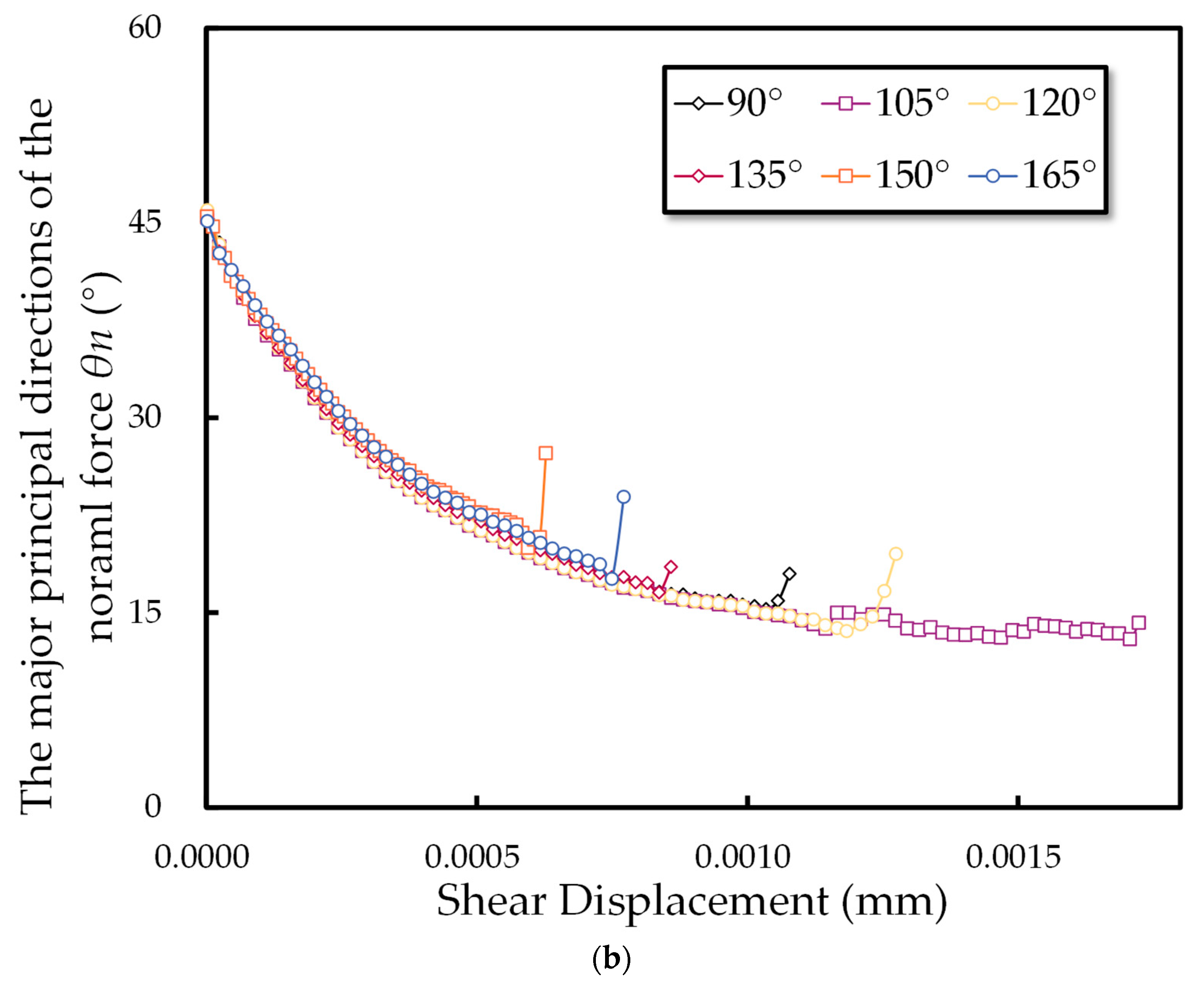
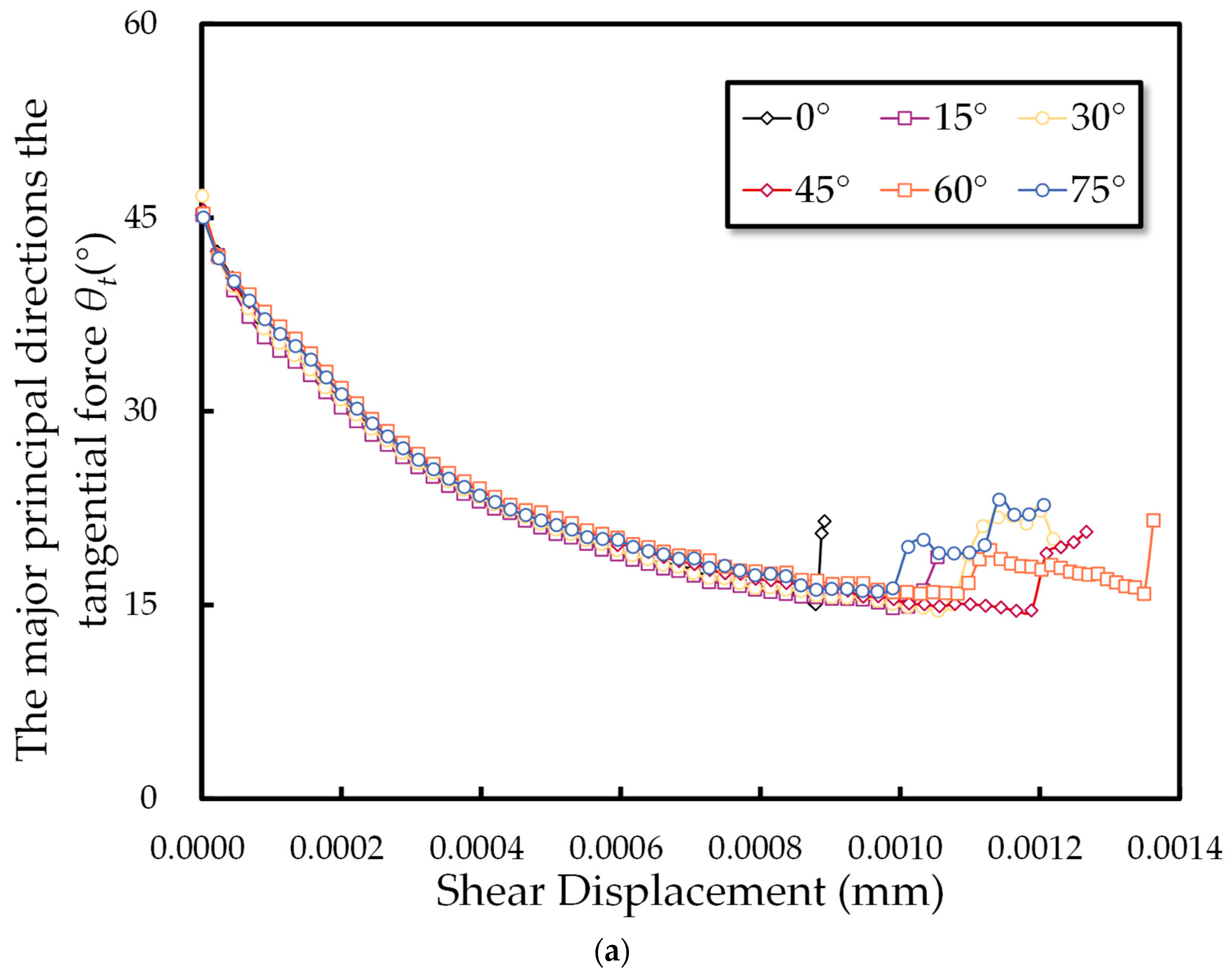
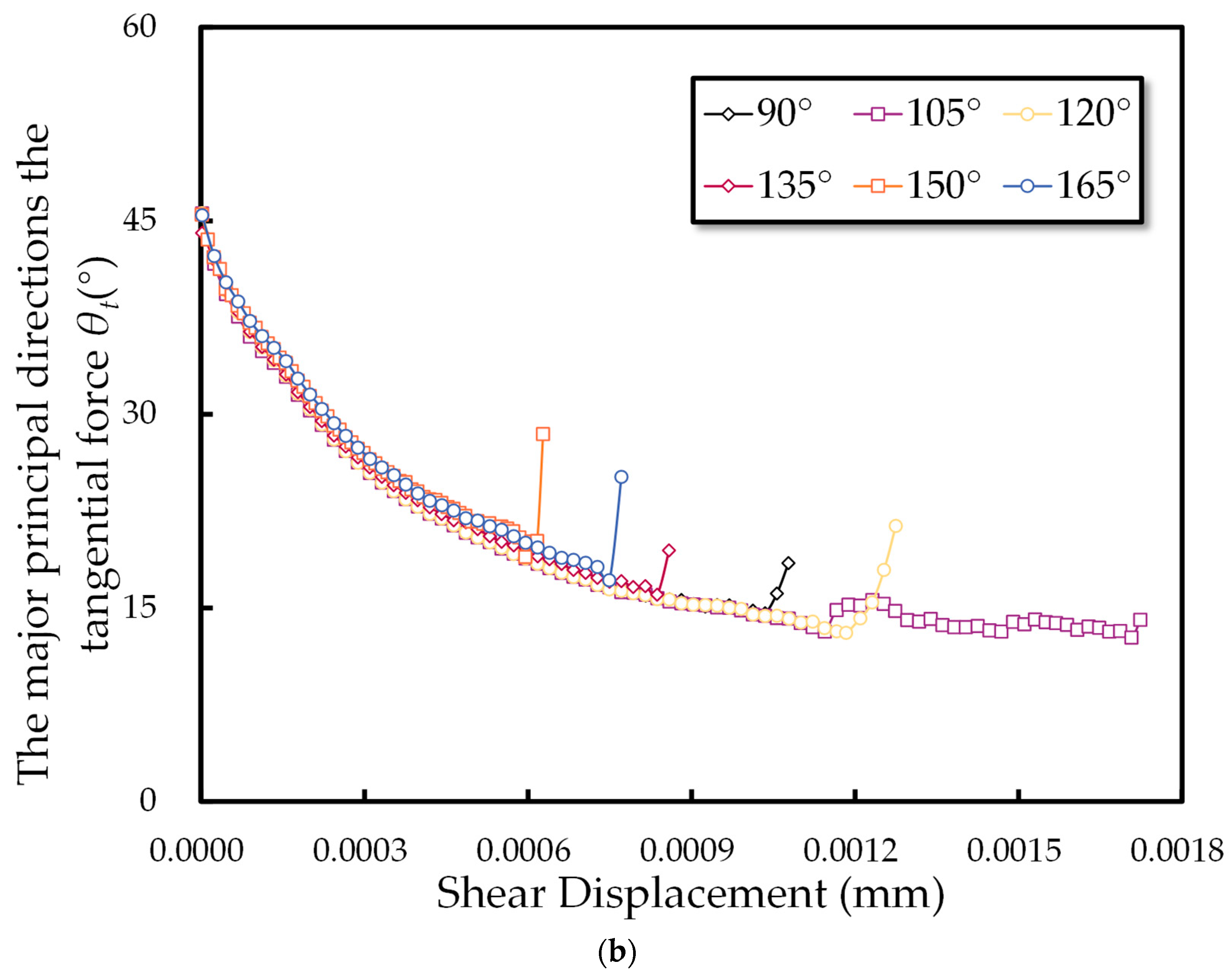
3.2.5. The Evolution of Major Principal Directions During the Numerical Experiment

In the process of shear, the direction of the contact force will be deflected; the study of the deflection of the main direction of the contact force is essential to understanding the force conduction mechanism and the damage mechanism of the specimen under the action of shear load. As shown in Figure 18 and Figure 19, the evolution of the major principal direction of normal and tangential forces is almost consistent, which is similar to the research results of Li et al. At the initial stage of loading, the main directions of normal and tangential forces are around 45 °, which is due to the isotropic compaction of the sample during the initial stage of loading. As the shear progresses, the deflection angle of the major directions of the normal and tangential forces continuously decreases; that is, the major direction continuously deviates towards the shear direction. After the specimen reaches its peak shear stress, microcracks aggregate and coalesce to form macroscopic cracks. The major directions of normal and tangential forces rapidly increase; that is, the major directions rapidly deviate from the shear direction, the contact between particles is broken, the energy stored in the contact is released, and the shear stress decreases. It is worth noting that, similarly to the variation trend of the coefficients a n and a t , before a large number of microcracks appear in the specimens, the major directions of normal and tangential forces in different specimens almost coincide. However, after the appearance of microcracks, there are varying degrees of deflection in the major direction. After the microcracks of the sample aggregate and penetrate, the main direction deviates from the loading direction. At the same time, a larger peak shear stress often corresponds to a greater deviation of the major directions of normal and tangential forces towards the loading axis, because the greater deflection angle mobilizes the ability to store energy in contact between particles.

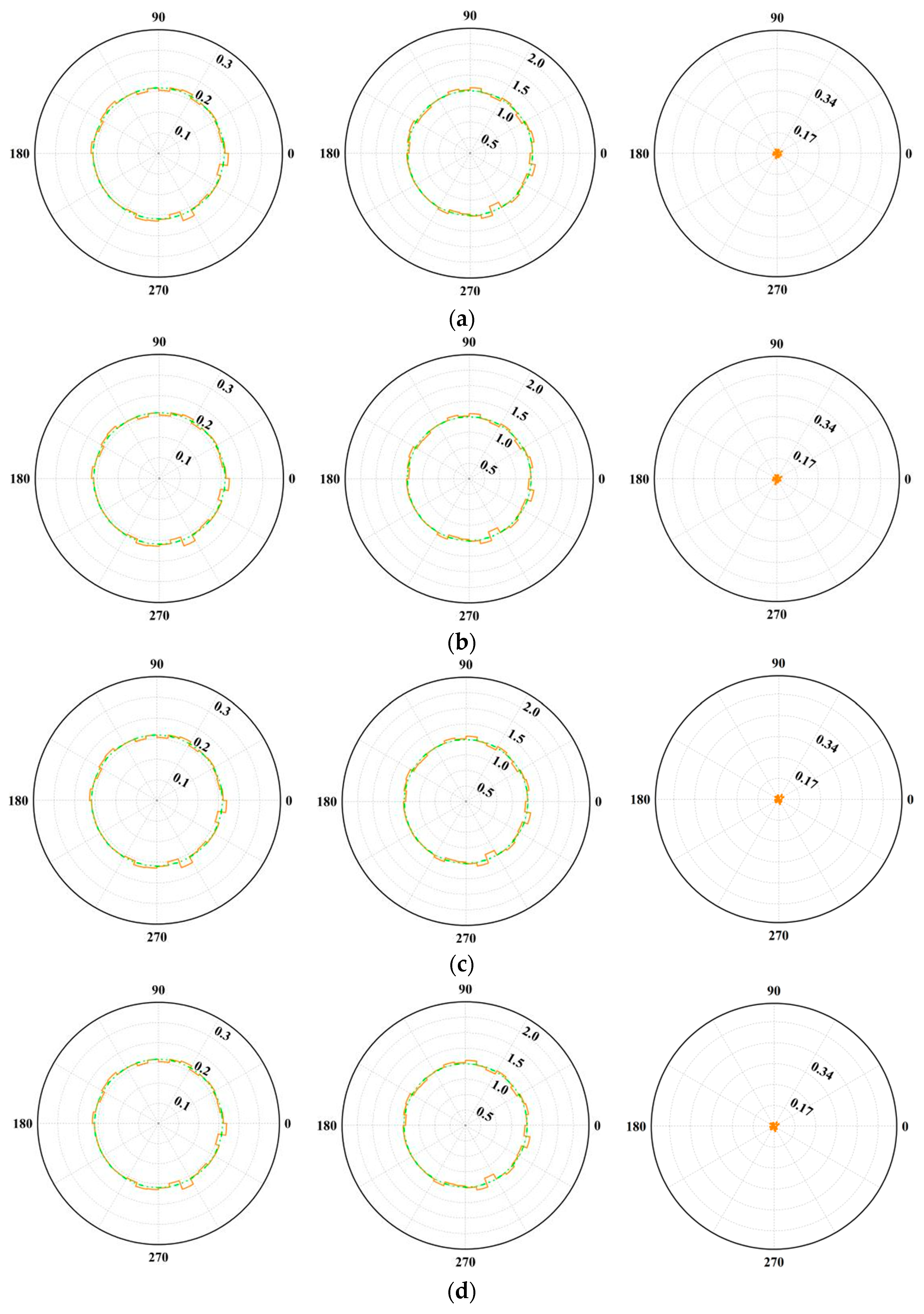
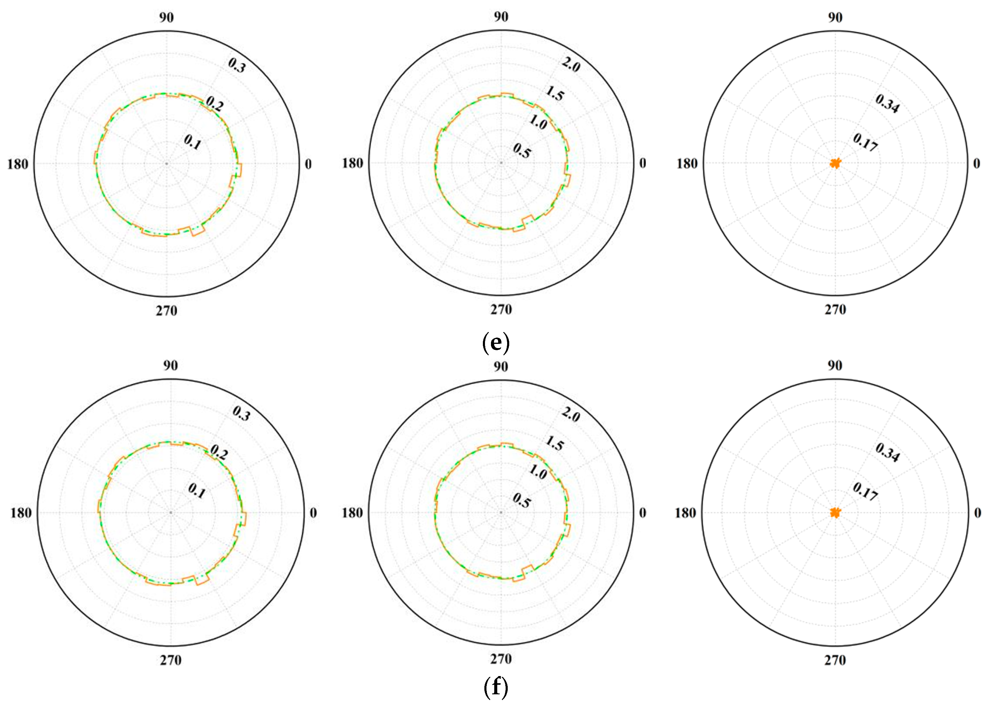
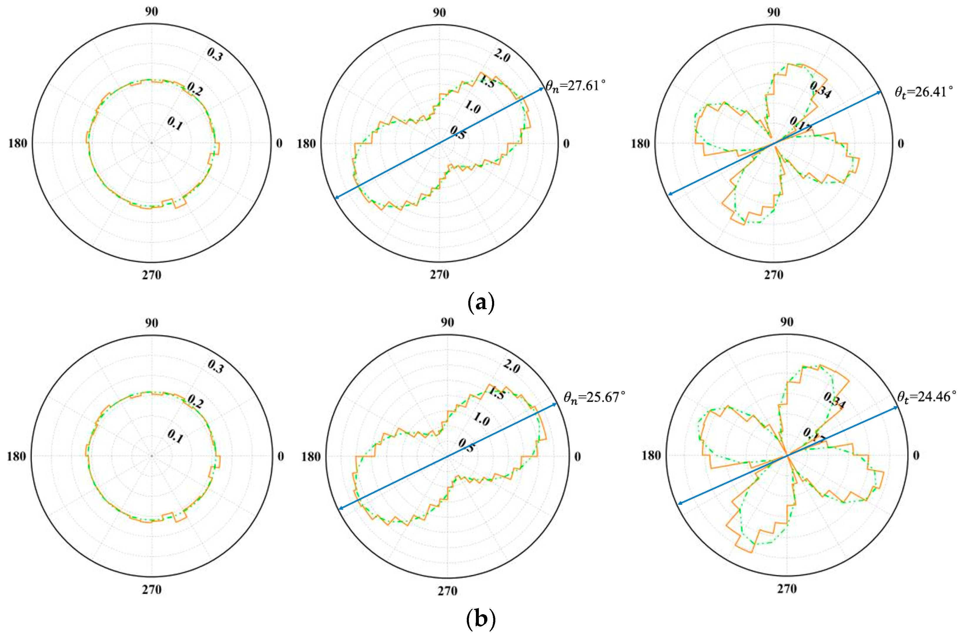
3.2.6. Anisotropic Distribution

Analyzing the evolution of anisotropy in direct shear tests across specimens with varying joint inclinations, a detailed examination of geometric and mechanical anisotropy through microstructural mechanisms offers insights into complex macro behaviors. This includes the topological organization of particle arrangements and the dynamics of internal force transfer. The study of polar distributions, encompassing contact fabric, normal force and shear force anisotropy in three distinct phases (initial, 50% pre peak, and post peak), elucidates the microstructural alterations during rock deformation. Additionally, this research incorporates numerical measurement data and distribution estimates derived from second-order tensor relationships (16), (26) and (27). These relationships are integral to quantifying the spatial positions of micromechanical elements like contact normals and forces.
Figure 20, Figure 21 and Figure 22 demonstrate that these second-order tensor models accurately mirror the measured data. It is noteworthy that the applied shear load fundamentally alters the initial anisotropy within the specimens. Upon comparison, the anisotropy distribution of contact normals appears more circular, signifying a lesser degree of anisotropy. This observation aligns with the a c distribution showed in Figure 15, suggesting a reduced a c value.
In the polar histogram of the contact normal force, the initial isotropic compaction of the specimens produces a nearly circular distribution, reflecting uniform contact forces in all directions. With progressive loading, this histogram morphs into a peanut-like shape, its long axis tilting towards the loading axis, as documented by [11,17,31]. Joint inclination significantly influences this pattern, as varying inclinations alter microcrack distribution under shear stress. Specimens with larger peak shear stresses typically exhibit more elongated normal force distribution histograms, with the longer axis more aligned with the loading direction.
Regarding the polar histogram of the contact tangential force, initial measurements are near zero across all specimens due to the absence of shear deformation during isotropic compaction. However, as shear stress is applied, the histogram displays a unique petal shape, marked by four distinct leaps, in contrast to the peanut shape of the normal force histogram. These leaps indicate the directions where high shear forces accumulate. Just as with the normal force, the predominant direction of tangential force anisotropy swiftly shifts to align with the loading axis.

4. Discussion

Through detailed discrete element method simulations, our comprehensive analysis of the mechanical behaviors and deformation mechanisms in rock masses under direct shear loading, considering different joint inclinations, has yielded insights into the evolution of energy, fabric and anisotropy in the contact direction and force.
Joint inclination significantly influences rock mechanics, which is primarily evident in microcrack formation within the samples. Variations in joint inclination result in distinct patterns of microcracks under shear stress, which in turn critically impacts friction-dominated plastic property dissipation. This factor is crucial to determining the failure mode of the rock mass, leading to either brittle or ductile failure. Moreover, joint inclination plays a role in the specimen’s capacity to store elastic energy. In particular, when joints are inclined oppositely to the loading direction and at steep angles, the formation of sawtooth-like tensile cracks is more likely, reducing the elastic energy storage. This storage capacity is a key determinant of the peak shear strength of the rock. The rock masses’ shear strength declines sharply when the strain and bonding energies stored within the internal contacts surpass the contacts’ load-bearing capacity.
As illustrated in Figure 10, while the fracture energy from microcracks in rocks consumes only a minor fraction of the total input energy, it induces permanent alterations in the overall microstructure of the rock masses. Notably, these changes are manifested in the evolution of the coordination number, fabric anisotropy, and contact force anisotropy. The proliferation of microcracks facilitates the gradual loosening of constraints between particles, potentially leading to positional shifts during structural rearrangement. Consequently, the coordination number, fabric anisotropy, and contact force anisotropy tend to decline over time, with a marked reduction upon the emergence of macroscopic cracks.
From a micromechanical standpoint, the strength of rock masses is reliant on their capacity to develop anisotropy. The mechanical anisotropy trends observed (refer to Figure 16 and Figure 17) align closely with the macroscopic stress trends depicted in Figure 4, a finding consistent with numerous laboratory and numerical studies. Moreover, changes in failure modes are intimately linked to micromechanical origins. Post-microcrack formation, a gradual increase in fabric and contact force anisotropy contributes to a larger displacement before the peak stress is reached, while a slower reduction post peak correlates with increased residual strength.

5. Conclusions

This investigation, utilizing discrete element method numerical simulations, explores the influence of joint inclination on the shear behavior of rock specimens. This includes examining shear deformation, failure modes, shear strength and energy evolution, along with the progression of fabric and mechanical anisotropy during shearing. The key findings are:
(1)
In the initial loading phase, the joint inclination angle has a minimal impact on deformability. However, it significantly affects the peak shear stress and peak displacement in rock masses, with the specific trends illustrated in Figure 5 and Figure 6.
(2)
Although fracture energy accounts for a minor proportion of the total input energy, it markedly alters the rock mass microstructure. Variations in joint inclination angles directly influence the formation and orientation of microcracks. These, in turn, have a decisive effect on peak displacement and the nature of failure brittle or ductile. Additionally, these angles impact the specimens’ capacity to store elastic energy, which is a crucial factor determining the peak shear stress of the rock-like specimens.
(3)
The progression of fabric and mechanical anisotropy at the microscopic level aligns with macroscopic deformation behaviors, as depicted in the shear stress–shear displacement curve. This correlation provides micromechanical substantiation and underscores the transition in rock mass failure modes with varying joint inclination angles. As the angle increases, the mode shifts from brittle to ductile, then reverts to brittle failure.
(4)
Changes in joint inclination angles not only influence the emergence of microcracks, impacting internal microstructure of the rock mass, but also significantly affect fabric and contact force anisotropy. Consistent with macroscopic deformation behavior, changes in fabric anisotropy and mechanical anisotropy provide micromechanical evidence; decreases in fabric anisotropy and contact anisotropy often signal specimen failure. Specimens displaying higher peaks in these anisotropies typically exhibit greater peak shear stress.
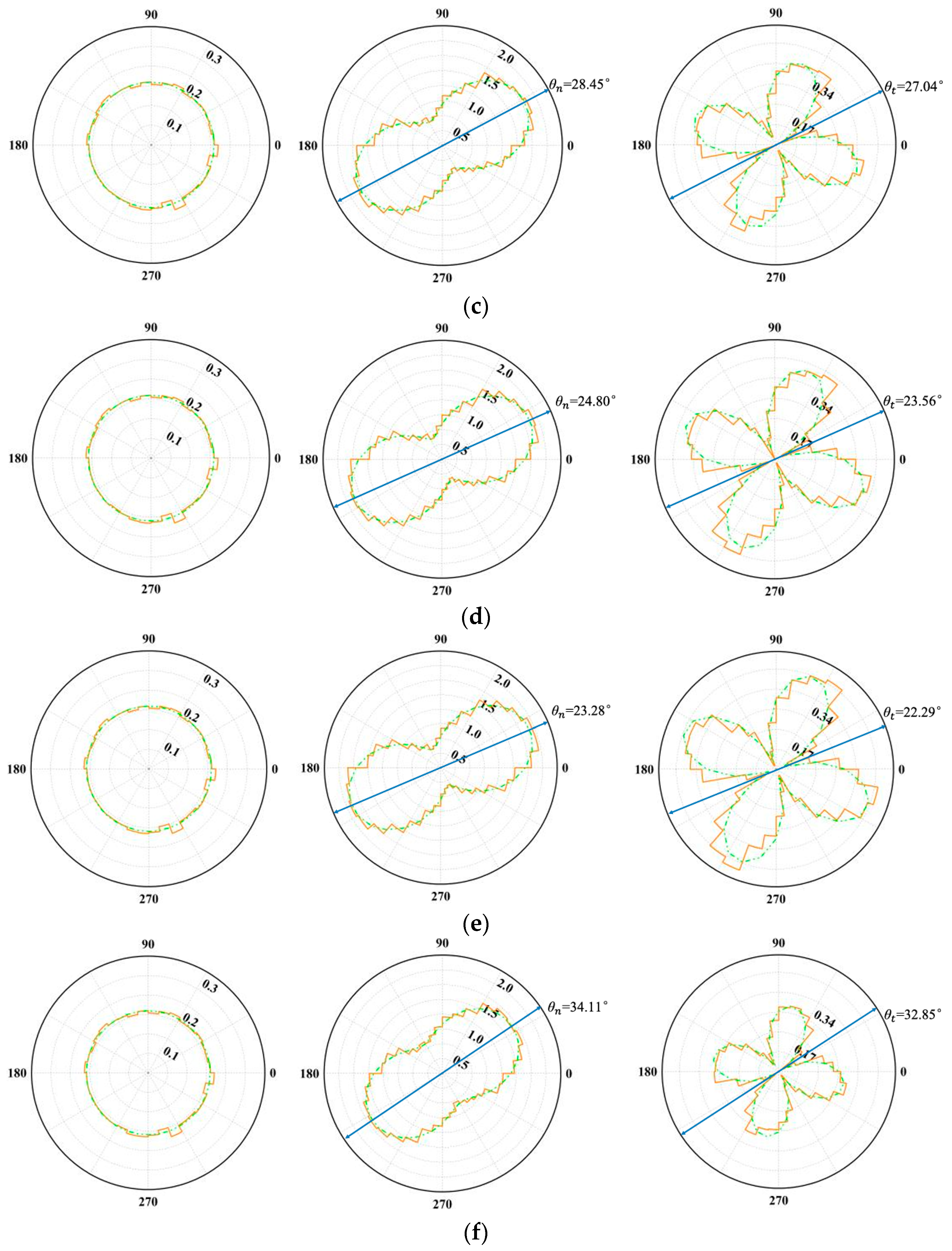
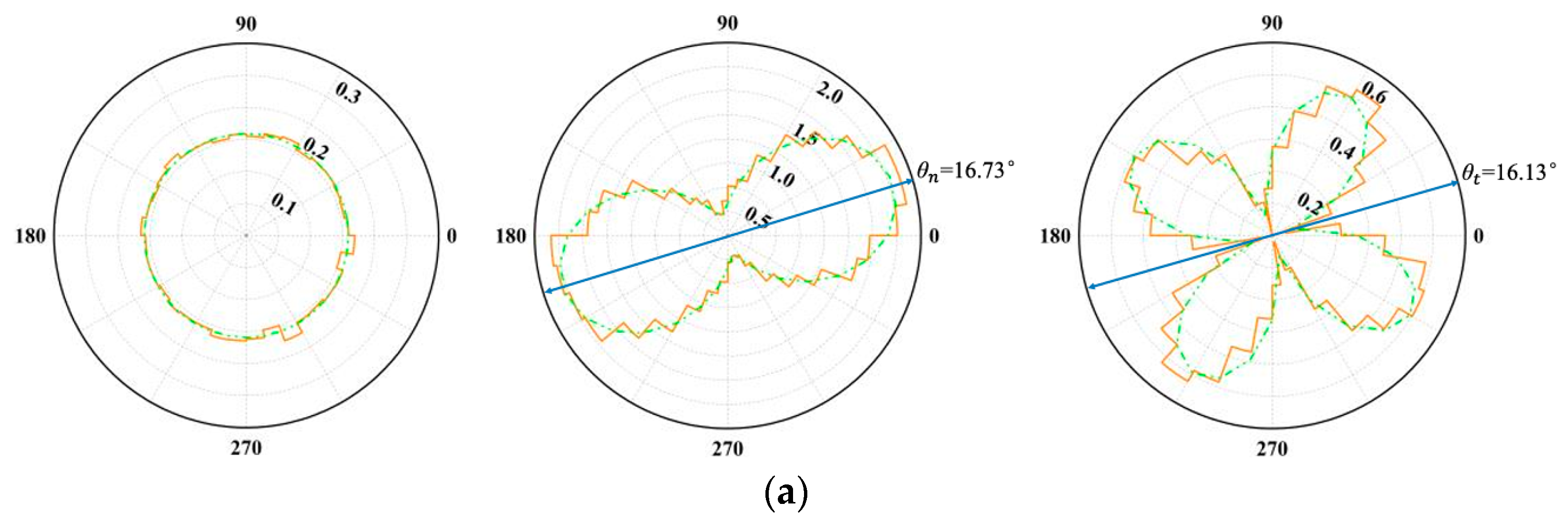
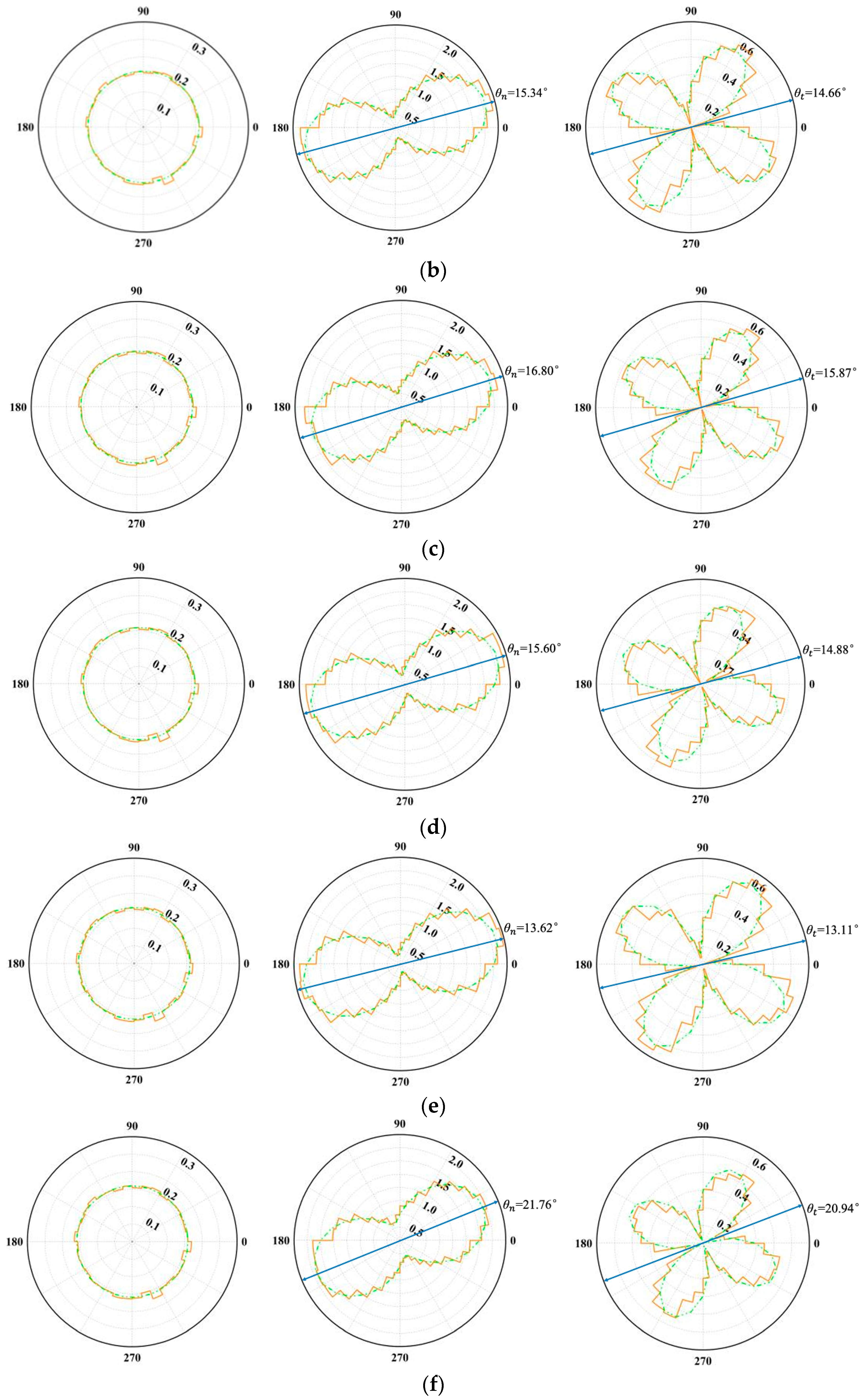
(5)
Polar histograms of the contact normal force often exhibit a “peanut-shaped” distribution, while those of the tangential force assume a four-lobed “petal-shaped” pattern. The approximation function presented in this study accurately captures these numerical measurement outcomes. Joint inclination plays a pivotal role in shaping these force distributions; specimens with higher peak shear stresses tend to show more pronounced, slender peanut shapes in a normal force distribution and more expansive petal shapes under tangential force, with the principal direction more closely aligned with the loading axis.

Author Contributions

Conceptualization, W.W. and L.S.; methodology, L.S.; software, K.Z.; validation, W.W., L.S. and G.S.; formal analysis, K.Z.; investigation, K.Z.; resources, W.W.; data curation, K.Z.; writing—original draft preparation, K.Z.; writing—review and editing, K.Z.; visualization, L.S.; supervision, W.W. and L.S.; project administration, L.S.; funding acquisition, L.S. All authors have read and agreed to the published version of the manuscript.

Funding

The research presented in this paper was supported by S&T Program of Hebei (23567602H).

Data Availability Statement

The raw data supporting the conclusions of this article will be made available by the authors on request.

Conflicts of Interest

The authors declare no conflicts of interest.

References

  1. Cheng, Y.; Wong, L.N.Y.; Zou, C. Experimental Study on the Formation of Faults from En-Echelon Fractures in Carrara Marble. Eng. Geol. 2015, 195, 312–326. [Google Scholar] [CrossRef]
  2. Huang, D.; Cen, D.; Ma, G.; Huang, R. Step-Path Failure of Rock Slopes with Intermittent Joints. Landslides 2015, 12, 911–926. [Google Scholar] [CrossRef]
  3. Zhang, K.; Chen, Y.; Fan, W.; Liu, X.; Luan, H.; Xie, J. Influence of Intermittent Artificial Crack Density on Shear Fracturing and Fractal Behavior of Rock Bridges: Experimental and Numerical Studies. Rock Mech. Rock Eng. 2020, 53, 553–568. [Google Scholar] [CrossRef]
  4. Shang, J.; West, L.J.; Hencher, S.R.; Zhao, Z. Geological Discontinuity Persistence: Implications and Quantification. Eng. Geol. 2018, 241, 41–54. [Google Scholar] [CrossRef]
  5. Lajtai, E.Z. Tensile Strength and Its Anisotropy Measured by Point and Line-Loading of Sandstone. Eng. Geol. 1980, 15, 163–171. [Google Scholar] [CrossRef]
  6. Gehle, C.; Kutter, H.K. Breakage and Shear Behaviour of Intermittent Rock Joints. Int. J. Rock Mech. Min. Sci. 2003, 40, 687–700. [Google Scholar] [CrossRef]
  7. Tang, P.; Chen, G.-Q.; Huang, R.-Q.; Zhu, J. Brittle Failure of Rockslides Linked to the Rock Bridge Length Effect. Landslides 2020, 17, 793–803. [Google Scholar] [CrossRef]
  8. Cao, R.H.; Yao, R.; Lin, H.; Lin, Q.B.; Meng, Q.; Li, T. Shear behaviour of 3D nonpersistent jointed rock-like specimens: Experiment and numerical simulation. Comput. Geotech. 2022, 148, 104858. [Google Scholar] [CrossRef]
  9. Nguyen, H.; Wang, J.; Bazilevs, Y. A smooth Crack-Band Model for anisotropic materials: Continuum theory and computations with the RKPM meshfree method. Int. J. Solids Struct. 2024, 288, 112618. [Google Scholar] [CrossRef]
  10. Zhang, Y.; Bažant, Z.P. Smooth Crack Band Model—A Computational Paragon Based on Unorthodox Continuum Homogenization. J. Appl. Mech. 2023, 90, 041007. [Google Scholar] [CrossRef]
  11. Gao, G.; Meguid, M.A.; Chouinard, L.E. On the Role of Pre-Existing Discontinuities on the Micromechanical Behavior of Confined Rock Samples: A Numerical Study. Acta Geotech. 2020, 15, 3483–3510. [Google Scholar] [CrossRef]
  12. Oda, M. Deformation Mechanism of Sand in Triaxial Compression Tests. Soils Found. 1972, 12, 45–63. [Google Scholar] [CrossRef] [PubMed]
  13. Oda, M.; Kazama, H.; Konishi, J. Effects of Induced Anisotropy on the Development of Shear Bands in Granular Materials. Mech. Mater. 1998, 28, 103–111. [Google Scholar] [CrossRef]
  14. Oda, M. Initial Fabrics and Their Relations to Mechanical Properties of Granular Material. Soils Found. 1972, 12, 17–36. [Google Scholar] [CrossRef]
  15. Oda, M. The Mechanism of Fabric Changes During Compressional Deformation of Sand. Soils Found. 1972, 12, 1–18. [Google Scholar] [CrossRef]
  16. Zhu, K.; Sun, G.; Shi, L. Shear-Induced Anisotropy Analysis of Rock Masses Containing Non-Coplanar Intermittent Joints. Arch. Appl. Mech. 2024, 94, 841–864. [Google Scholar] [CrossRef]
  17. Gao, G.; Meguid, M.A. Microscale Characterization of Fracture Growth in Increasingly Jointed Rock Samples. Rock Mech. Rock Eng. 2022, 55, 6033–6061. [Google Scholar] [CrossRef]
  18. Guo, N.; Zhao, J. The Signature of Shear-Induced Anisotropy in Granular Media. Comput. Geotech. 2013, 47, 1–15. [Google Scholar] [CrossRef]
  19. Tai, D.; Qi, S.; Zheng, B.; Wang, C.; Guo, S.; Luo, G. Shear Mechanical Properties and Energy Evolution of Rock-like Samples Containing Multiple Combinations of Non-Persistent Joints. J. Rock Mech. Geotech. Eng. 2022, 15, 1651–1670. [Google Scholar] [CrossRef]
  20. Qi, S.; Zheng, B.; Wu, F.; Huang, X.; Guo, S.; Zhan, Z.; Zou, Y.; Barla, G. A New Dynamic Direct Shear Testing Device on Rock Joints. Rock Mech. Rock Eng. 2020, 53, 4787–4798. [Google Scholar] [CrossRef]
  21. Sarfarazi, V.; Ghazvinian, A.; Schubert, W.; Blumel, M.; Nejati, H.R. Numerical Simulation of the Process of Fracture of Echelon Rock Joints. Rock Mech. Rock Eng. 2014, 47, 1355–1371. [Google Scholar] [CrossRef]
  22. Zhang, X.-P.; Wong, L.N.Y. Cracking Processes in Rock-Like Material Containing a Single Flaw Under Uniaxial Compression: A Numerical Study Based on Parallel Bonded-Particle Model Approach. Rock Mech. Rock Eng. 2011, 45, 711–737. [Google Scholar] [CrossRef]
  23. Xing, L.; Gong, W.; Li, B.; Zhao, C.; Tang, H.; Wang, L. Probabilistic Analysis of Earthquake-Induced Failure and Runout Behaviors of Rock Slopes with Discrete Fracture Network. Comput. Geotech. 2023, 159, 105487. [Google Scholar] [CrossRef]
  24. Chen, M.; Yang, S.-Q.; Ranjith, P.G.; Zhang, Y.-C. Cracking Behavior of Rock Containing Non-Persistent Joints with Various Joints Inclinations. Theor. Appl. Fract. Mech. 2020, 109, 102701. [Google Scholar] [CrossRef]
  25. Lin, Q.; Cao, P.; Liu, Y.; Cao, R.; Li, J. Mechanical Behaviour of a Jointed Rock Mass with a Circular Hole under Compression-Shear Loading: Experimental and Numerical Studies. Theor. Appl. Fract. Mech. 2021, 114, 102998. [Google Scholar] [CrossRef]
  26. Xie, H.; Li, L.; Peng, R.; Ju, Y. Energy Analysis and Criteria for Structural Failure of Rocks. J. Rock Mech. Geotech. Eng. 2009, 1, 11–20. [Google Scholar] [CrossRef]
  27. Luo, Y.; Wang, G.; Li, X.; Liu, T.; Mandal, A.K.; Xu, M.; Xu, K. Analysis of Energy Dissipation and Crack Evolution Law of Sandstone under Impact Load. Int. J. Rock Mech. Min. Sci. 2020, 132, 104359. [Google Scholar] [CrossRef]
  28. Satake, M. Fundamental Quantities in the Graph Approach to Granular Materials. In Studies in Applied Mechanics; Elsevier: Amsterdam, The Netherlands, 1983; Volume 7, pp. 9–19. ISBN 978-0-444-42192-0. [Google Scholar]
  29. Silbert, L.E.; Grest, G.S.; Landry, J.W. Statistics of the Contact Network in Frictional and Frictionless Granular Packings. Phys. Rev. E 2002, 66, 061303. [Google Scholar] [CrossRef] [PubMed]
  30. Oda, M. Co-Ordination Number and Its Relation to Shear Strength of Granular Material. Soils Found. 1977, 17, 29–42. [Google Scholar] [CrossRef] [PubMed]
  31. Li, X. Micro-Scale Investigation on the Quasi-Static Behavior of Granular Material. Ph.D. Thesis, The Hong Kong University of Science and Technology, Hong Kong, China, 2006. [Google Scholar]
  32. Li, X.; Yu, H.-S. On the Stress–Force–Fabric Relationship for Granular Materials. Int. J. Solids Struct. 2013, 50, 1285–1302. [Google Scholar] [CrossRef]
  33. Ken-Ichi, K. Distribution of Directional Data and Fabric Tensors. Int. J. Eng. Sci. 1984, 22, 149–164. [Google Scholar] [CrossRef]
  34. Li, X.; Yu, H.S. Tensorial Characterisation of Directional Data in Micromechanics. Int. J. Solids Struct. 2011, 48, 2167–2176. [Google Scholar] [CrossRef]
  35. Guo, N. Multiscale Characterization of the Shear Behavior of Granular Media. Ph.D. Thesis, The Hong Kong University of Science and Technology, Hong Kong, China, 2014; p. b1334193. [Google Scholar]
  36. Xu, W.; Ren, W.; Liu, Y.; Liu, C.; Cai, S. Micromechanical Behavior of Jointed Rock Masses under Uniaxial Compression Loading: A Numerical Study Based on the Discrete Element Method. Eur. J. Environ. Civil. Eng. 2022, 27, 3653–3678. [Google Scholar] [CrossRef]
Figure 1. The geometrical parameters of the non-persistent joints. l—rock bridge length; b—joint length; α —joint inclination (around the midpoint of the joint).
Mathematics 13 00362 g001
Figure 2. Shear stress versus the displacement curves of numerical tests with 0° joint angles under a normal force of 2.5 kN compared with the results of laboratory tests.
Mathematics 13 00362 g002
Figure 3. Arrangement of models with different joint inclinations. (a) A0°, (b) A15°, (c) A30°, (d) A45°, (e) A60°, (f) A75°, (g) A90°, (h) A105°, (i) A120°, (j) A135°, (k) A150°, (l) A165°.
Mathematics 13 00362 g003aMathematics 13 00362 g003b
Figure 7. Microcrack propagation of specimens containing different joint inclinations. (a) A0°, (b) A15°, (c) A30°, (d) A45°, (e) A60°, (f) A75°, (g) A90°, (h) A105°, (i) A120°, (j) A135°, (k) A150°, (l) A165°.
Mathematics 13 00362 g007
Figure 8. Shear stress–shear displacement responses and cumulative microcrack–shear displacement curves for different joint inclinations. (a) A0°, (b) A15°, (c) A30°, (d) A45°, (e) A60°, (f) A75°, (g) A90°, (h) A105°, (i) A120°, (j) A135°, (k) A150°, (l) A165°.
Mathematics 13 00362 g008aMathematics 13 00362 g008bMathematics 13 00362 g008c
Figure 9. Energy–shear displacement responses of different joint inclination specimens. (a) A0°, (b) A15°, (c) A30°, (d) A45°, (e) A60°, (f) A75°, (g) A90°, (h) A105°, (i) A120°, (j) A135°, (k) A150°, (l) A165°.
Mathematics 13 00362 g009aMathematics 13 00362 g009b
Figure 10. Energy partitioning into elastic energy and plastic energy when the rock specimens reach their peak strength.
Mathematics 13 00362 g010
Figure 11. The deviatoric fabric for specimens with different joint inclinations considering all engaged contacts. (a) A0–A75°, (b) A90–A165°.
Mathematics 13 00362 g011
Figure 12. The deviatoric fabric for specimens with different joint inclinations considering contacts that only transmit compressive force. (a) A0–A75°, (b) A90–A165°.
Mathematics 13 00362 g012
Figure 13. The deviatoric fabric for specimens with different joint inclinations considering contacts that only transmit tensile force. (a) A0–A75°, (b) A90–A165°.
Mathematics 13 00362 g013
Figure 14. The coordination number for specimens with different joint inclinations. (a) A0–A75°, (b) A90–A165°.
Mathematics 13 00362 g014aMathematics 13 00362 g014b
Figure 15. The evolution of geometric anisotropy ac with the shear displacement for different joint inclination specimens. (a) A0–A75°, (b) A90–A165°.
Mathematics 13 00362 g015
Figure 16. The evolution of mechanical anisotropy an with the shear displacement for different joint inclination specimens. (a) A0–A75°, (b) A90–A165°.
Mathematics 13 00362 g016
Figure 17. The evolution of mechanical anisotropy at with the shear displacement for different joint inclination specimens. (a) A0–A75°, (b) A90–A165°.
Mathematics 13 00362 g017
Figure 18. The evolution of the major principal direction of the normal force θ n with the shear displacement in different joint inclination specimens. (a) A0–A75°, (b) A90–A165°.
Mathematics 13 00362 g018aMathematics 13 00362 g018b
Figure 19. The evolution of the major principal direction of the tangential force θ t with the shear displacement in different joint inclination specimens. (a) A0–A75°, (b) A90–A165°.
Mathematics 13 00362 g019aMathematics 13 00362 g019b
Figure 20. The distribution of anisotropies of the contact normal ( E c ( n i ) ), the normalized average contact normal force ( f ¯ n Θ / f ¯ 0 ) and the normalized average contact shear force ( f ¯ t Θ / f ¯ 0 ) for the different joint inclination specimens at the initial stress state: (a) A0°, (b) A30°, (c) A60°, (d) 90°, (e) A120°, (f) A150°.
Mathematics 13 00362 g020aMathematics 13 00362 g020b
Figure 21. The distribution of the anisotropies of the contact normal ( E c ( n i ) ), normalized average contact normal force ( f ¯ n Θ / f ¯ 0 ) and normalized average contact shear force ( f ¯ t Θ / f ¯ 0 ) for the different joint inclination specimens at the 50% peak stress state: (a) A0°, (b) A30°, (c) A60°, (d) 90°, (e) A120°, (f) A150°.
Mathematics 13 00362 g021aMathematics 13 00362 g021b
Figure 22. The distribution of the anisotropies of the contact normal ( E c ( n i ) ), normalized average contact normal force ( f ¯ n Θ / f ¯ 0 ) and normalized average contact shear force ( f ¯ t Θ / f ¯ 0 ) for the different joint inclination specimens at the peak stress state: (a) A0°, (b) A30°, (c) A60°, (d) 90°, (e) A120°, (f) A150°.
Mathematics 13 00362 g022aMathematics 13 00362 g022b
Table 1. Mechanical properties of rock-like material.
Fundamental Mechanical ParametersValue
Density, ρ   (kg/m3)1.32
Young’s modulus, E (GPa)5.78
Uniaxial compressive strength, σ c   (MPa)9.22
Cohesion, c (MPa)0.523
Friction angle, φ   (°)59
Table 2. Microscopic parameters used in the discrete element analysis.
MaterialsItemMicromechanical Properties
RockBall–ball contact effective modulus ( E c )0.22 GPa
Ball stiffness ratio ( k n / k s )1.1
Ball friction coefficient ( μ )0.3
Parallel-bond effective modulus ( E ¯ c )0.22 GPa
Parallel-bond stiffness ratio ( k ¯ n / k ¯ s )1.1
Parallel-bond tensile strength ( σ ¯ t )2.8 MPa
Parallel-bond cohesion ( c ¯ )2.2 MPa
JointSmooth-joint normal stiffness ( k n s j )1000 GPa/m
Smooth-joint shear stiffness ( k s s j )500 GPa/m
Smooth-joint friction coefficient ( μ s j )0.2
Smooth-joint tensile strength ( σ t s j )0 MPa
Smooth-joint cohesion ( c s j )0 MPa
Disclaimer/Publisher’s Note: The statements, opinions and data contained in all publications are solely those of the individual author(s) and contributor(s) and not of MDPI and/or the editor(s). MDPI and/or the editor(s) disclaim responsibility for any injury to people or property resulting from any ideas, methods, instructions or products referred to in the content.

