A Surrogate Model for the Rapid Prediction of Factor of Safety in Slopes with Spatial Variability

Abstract

Due to the complexity and long-term nature of geological evolution, geotechnical strength parameters exhibit significant spatial variability, which has a crucial impact on slope stability assessment. While traditional numerical methods combined with Monte Carlo simulations and Gaussian random field theory provide accurate stability analysis, their high computational cost makes them impractical for large-scale engineering applications. To address this issue, this study proposes an efficient surrogate modeling approach for the rapid prediction of the factor of safety in slopes while considering the spatial variability of geotechnical parameters. The accuracy and robustness of the proposed model are validated through a single-layer slope case study. Results demonstrate that this approach not only ensures computational accuracy but also significantly enhances efficiency. Compared with conventional methods, the surrogate model effectively replaces high-cost numerical simulations, offering a practical and efficient solution for slope stability analysis under complex geological conditions, with high potential for engineering applications.

1. Introduction

The mechanical behavior of geomaterials is inherently governed by the complexity and prolonged timescale of geological evolution. Over millions of years, geomaterials undergo intricate processes such as sedimentation, chemical weathering, material transport, and stress redistribution. These processes introduce anisotropy, heterogeneity, and randomness in geomechanical properties, further exacerbated by tectonic activities, erosion, and diagenesis [1,2]. Even within the same geological formation, significant spatial variability is observed in key parameters, including cohesion and internal friction angle [3]. Consequently, the accurate quantification of spatial variability is essential for reliable slope stability assessments. Failure to incorporate this variability may lead to non-conservative safety predictions, increasing the risk of unexpected slope failures [4]. Thus, characterizing the spatial variability of geotechnical parameters and efficiently evaluating slope stability under such uncertainties has become a critical challenge in geotechnical engineering.

Within the framework of stochastic field theory, spatial variability can be systematically described using stochastic field models [5]. Among these, the Gaussian random field (GRF) is widely employed for spatial discretization of geotechnical parameters due to its strong adaptability to multiple parameters and mathematical tractability. The GRF characterizes spatial correlation structures using an autocorrelation function and enables numerical simulations through discretization techniques such as covariance matrix decomposition and spectral representation methods. To ensure physically meaningful, non-negative material properties, it is often assumed that geotechnical parameters follow a log-normal distribution [6,7]. The Cholesky decomposition method, owing to its high computational efficiency, straightforward implementation, and independence from field morphology, has been extensively utilized for GRF discretization in geotechnical modeling [8].

In slope stability analysis, conventional numerical methods based on the strength reduction method (SRM) require extensive iterative computations to determine the factor of safety (Fs) [9,10,11,12,13,14]. This process involves progressive strength reduction, nonlinear convergence criteria, and mesh dependency issues, leading to prohibitively high computational costs [15,16,17]. As a result, applying SRM to large-scale slope systems or conducting probabilistic stability analyses remains computationally challenging, limiting its feasibility for practical engineering applications. To mitigate these computational challenges, researchers have explored various surrogate modeling techniques to approximate numerical simulations with significantly reduced computational effort. These models leverage machine learning and regression-based approaches to establish input-output relationships from precomputed datasets. For instance, Su et al. [18] proposed an active learning-based reliability analysis framework that adaptively refines training samples to enhance computational efficiency, while Zhang et al. [19] introduced an explicit surrogate model to approximate Fs under different geotechnical conditions. Hu et al. [20] and Karniadakis et al. [21] achieved notable progress in applying physics-informed neural networks (PINNs) to constitutive modeling, inverse problems, and the identification, evaluation, and prediction of damage in solid materials and structures. Their work demonstrates the capability of physics-informed learning to uncover hidden physical laws and solve high-dimensional problems in both forward and inverse settings.

Although these methods have demonstrated considerable improvements in computational efficiency, they often fail to fully account for the spatial variability of geotechnical parameters. Neglecting spatial variability may introduce biases in stability assessments, particularly in heterogeneous soil and rock formations, thereby limiting the applicability of surrogate models under complex geological conditions. To incorporate the effects of spatial variability on slope stability, conventional numerical approaches are often coupled with Monte Carlo simulations (MCS) to analyze the probability distribution of Fs [22,23,24,25,26]. MCS enables probabilistic slope stability assessment by generating multiple realizations of spatially variable geotechnical parameters and performing SRM-based stability calculations for each realization. However, the need to conduct thousands of numerical simulations significantly amplifies computational demands, making MCS computationally prohibitive for large-scale applications.

To address this challenge, this study proposes a novel surrogate model capable of rapidly predicting Fs while explicitly considering spatial variability in geotechnical properties. The proposed model integrates spatially correlated random fields as input and employs a data-driven learning approach to approximate the complex relationship between geotechnical heterogeneity and slope stability. A single-layer slope case is used to validate the model’s accuracy and robustness. The results demonstrate that the proposed method significantly enhances computational efficiency while maintaining high predictive accuracy. By providing a balance between computational cost and prediction reliability, this approach offers a practical and efficient solution for slope stability assessment in geotechnical engineering, particularly in the presence of complex geological conditions.

2. Characterization of Spatial Variability in Geomaterials

2.1. Spatial Variability of Geotechnical Parameters

In geotechnical materials, physical and mechanical properties at different points are not independent but exhibit spatial correlation, meaning that adjacent regions tend to share similar characteristics. This correlation is typically quantified using an autocorrelation function, which describes the spatial dependence between any two points. Among various autocorrelation functions, the Gaussian autocorrelation function is widely adopted due to its smoothness and differentiability, facilitating the stable discretization of random fields [27]. Therefore, this study employs the Gaussian autocorrelation function as the basis for random field simulation, expressed as follows:

$$\rho ({\tau }_x,{\tau }_y)=\exp \left[-2\sqrt{{\left({\displaystyle \frac{{\tau }_x}{{\delta }_{\mathrm{h}}}}\right)}^2+{\left({\displaystyle \frac{2{\tau }_y}{{\delta }_v}}\right)}^2}\right]$$

(1)

where $\rho ({\tau }_x,{\tau }_y)$ is the autocorrelation coefficient between two points, ${\delta }_{\mathrm{h}}$ and ${\delta }_v$ represent the horizontal and vertical scales of fluctuation, respectively, ${\tau }_x$ and ${\tau }_y$ denote the horizontal and vertical distances between the two points.

2.2. Simulation of Spatially Variable Geotechnical Parameters Based on Cholesky Decomposition

The lognormal random field ${\mathit{\chi }}_B^{LN}(x,y)$, derived using the probability transformation method [28], can be expressed as

$${\mathit{\chi }}_B^{LN}(x,y)=\exp [{\mu }_{\ln B}+{\sigma }_{\ln B}{\mathit{\chi }}_B^G(x,y)]$$

(2)

where ${\mu }_{\ln B}$ and ${\sigma }_{\ln B}$ are the mean and standard deviation of the Gaussian random field, respectively, ${\sigma }_{\ln B}=\sqrt{\ln [1+{({\sigma }_B/{\mu }_B)}^2]}$, ${\mu }_{\ln B}=\ln {\mu }_B-{\sigma }_{\ln B}^2/2$; while ${\mu }_B$ and ${\sigma }_B$ represent the mean and standard deviation of the soil property $B$, which can include parameters such as cohesion $\mathrm{c}$ and internal friction angle $\phi$. The standard Gaussian random field ${\mathit{\chi }}_B^G(x,y)$ is given by

$${\mathit{\chi }}_B^G(x,y)={\mathit{L}}_2{\xi }_B{\mathit{L}}_1^T(B=c,\phi )$$

(3)

where ${\xi }_B$ is a vector of independent standard normal random variables, ${\mathit{L}}_1$ is obtained through Cholesky decomposition $\eta ={\mathit{L}}_1{\mathit{L}}_1^T$ of the cross-correlation matrix $\eta$. ${\mathit{L}}_2$ is obtained through Cholesky decomposition $C={\mathit{L}}_2{\mathit{L}}_2^T$ of the cross-correlation matrix $C$. The autocorrelation matrix $C$ is derived from the autocorrelation function and can be expressed as

$$\mathit{C}=\left[\begin{array}{cccc}1& \rho ({\tau }_{x_{1,2}},{\tau }_{y_{1,2}})& \cdots & \rho ({\tau }_{x_{1,n}},{\tau }_{y_{1,n}})\\ \rho ({\tau }_{x_{2,1}},{\tau }_{y_{2,1}})& 1& \cdots & \rho ({\tau }_{x_{2,n}},{\tau }_{y_{2,n}})\\ ⋮& ⋮& \ddots & ⋮\\ \rho ({\tau }_{x_{n,1}},{\tau }_{y_{n,1}})& \rho ({\tau }_{x_{n,2}},{\tau }_{y_{n,2}})& \cdots & 1\end{array}\right]$$

(4)

This formulation ensures that the generated random field preserves the spatial correlation characteristics of geotechnical parameters, providing a more realistic representation of material variability.

3. A Surrogate Model for the Rapid Prediction of Factor of Safety in Slopes with Spatial Variability

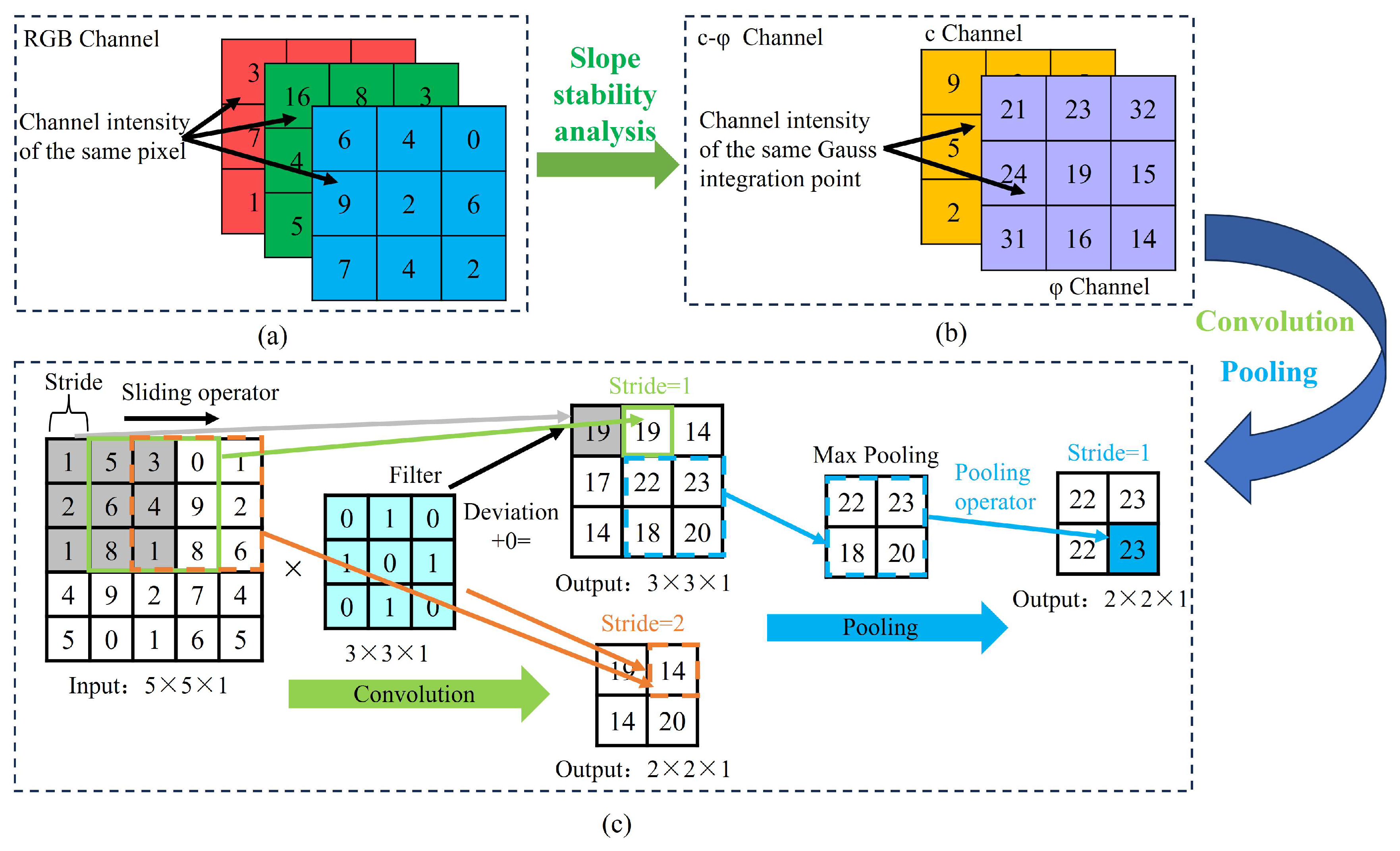
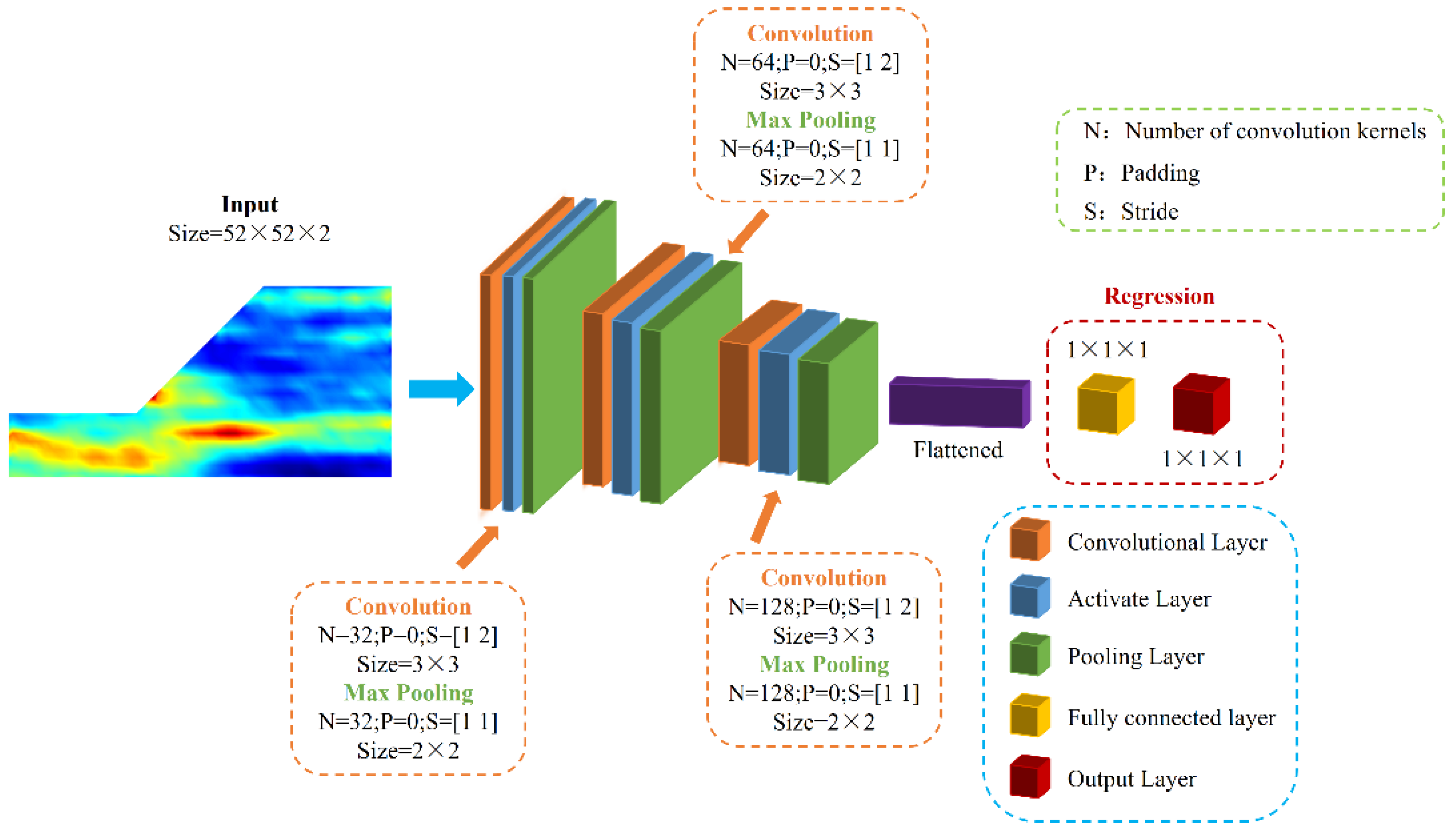
3.1. CNN-Based Surrogate Model

To efficiently predict the Fs of slopes, this study develops a surrogate model based on a convolutional neural network (CNN) algorithm. CNN is a deep learning model specifically designed for processing data with spatial topology, making it highly effective in extracting critical spatial features for slope stability analysis. The proposed model consists of several key layers, including the input layer, convolutional layers, pooling layers, activation layers, and normalization layers. These layers are typically followed by fully connected layers, dropout layers, and an output layer, forming a complete CNN architecture [29,30,31,32,33].

The input layer architecture of the proxy model for predicting the F_s of slopes differs from the approach used in conventional CNN designed for processing RGB digital images. In conventional CNN, RGB images are composed of pixels, where each pixel contains three intensity values corresponding to the red (R), green (G), and blue (B) color channels. As illustrated in Figure 1a, when processing such images, the input layer of a CNN is typically structured as 3 × 3 × 3, where the first two dimensions (3 × 3) represent the spatial resolution (width and height) of the input patch, and the third dimension (3) corresponds to the three RGB color channels. This multi-channel representation enables CNN to extract spatial and color-related features effectively.

In contrast, in numerical slope stability analysis, the soil strength parameters of the slope are assigned to Gauss integration points within the discretized mesh. When using CNN to analyze spatially variable slope random fields, these Gauss integration points can be treated similarly to pixels in conventional image processing. As illustrated in Figure 1b, drawing inspiration from how CNN handle RGB image channels, this study defines cohesion ($c$) and internal friction angle ($\phi$) as two independent channels, where each channel represents the values of cohesion and internal friction angle at the Gauss integration points, analogous to intensity values in RGB image channels. Therefore, in the CNN-based surrogate model for slope stability analysis, the input layer can be conceptualized as a two-channel “$c-\phi$ image”, where one channel corresponds to the spatial distribution of cohesion, and the other represents the spatial distribution of the internal friction angle. CNN then processes this dual-channel representation to predict the F_s. As shown in Figure 1b, the input size of the CNN-based surrogate model for slope stability analysis is set to 3 × 3 × 2, where the first two dimensions (3 × 3) denote the number of Gauss integration points in the width and height directions of the 2D computational domain, and the last dimension (2) represents the two random variables, $c$ and $\phi$.

In CNN-based slope stability analysis, the convolutional and pooling layers play a crucial role in extracting key features from the input data. For the convolution operation, let a sub-region of the input feature map be denoted by $X$, and let the corresponding convolution kernel (filter) weights be represented by $W$. The convolution process can then be formulated as

$$Y(i,j,e)={\displaystyle \sum _{m=0}^{K-1}{\displaystyle \sum _{n=0}^{K-1}{\displaystyle \sum _{d=0}^{D-1}X(i+m,j+n,d)\cdot W(m,n,d,e)+b_e}}}$$

(5)

where $X(i,j,d)$ is the value of the input feature at position $(i,j)$ in the $d$ th input channel, $W(m,n,d,e)$ denotes the weight of the convolution kernel at position $(m,n)$ for the $c$ th output channel, $b_e$ is the bias associated with the $e$ th output channel, $K$ is the size of the convolution kernel, $D$ is the number of input channels, and $e$ represents the number of output channels.

As shown in Figure 1c, the convolutional layer applies a sliding convolutional kernel (weight matrix) to perform local scanning across the input feature map, extracting and aggregating local features to capture spatial dependencies. As illustrated in Figure 1c, consider a convolution operation with a stride of 1. The first shaded subregion undergoes a dot product computation with the convolutional kernel, yielding a result of 19, which is assigned to the first cell of the output feature matrix. The kernel then shifts one step to the right (as indicated by the green box), and the same convolution operation produces another 19, which is placed in the second cell of the output matrix. When the stride is increased to 2, the output matrix dimensions are reduced to 2 × 2 × 1, demonstrating a lower resolution representation of the input features. In this case, the first computed value remains 19, while the second value is 14 (highlighted by the orange box), reflecting the different receptive fields covered by the kernel at this stride setting.

The pooling layer is designed to perform feature compression, reducing the spatial resolution of feature maps while preserving essential information. This process enhances the model’s ability to capture global patterns and mitigates the risk of overfitting by preventing the network from becoming overly sensitive to local variations. Common pooling methods include max pooling and average pooling, with this study adopting the max pooling strategy due to its effectiveness in retaining the most significant features. The pooling operation is similar to convolution, where a sliding pooling window moves across the input feature matrix and applies an aggregation function within each window. The mathematical formulation of the max-pooling operation is expressed as follows:

$$Y(i,j,e)=\underset{(m,n)\in R}{\max }X(i+m,j+n,e)$$

(6)

where $X(i,j,e)$ denotes the value of the input feature map at position $(i,j)$ in the $e$th channel, $Y(i,j,e)$ represents the output value after pooling, and $R$ denotes the receptive field of the max-pooling operator. The max operation selects the maximum value within the defined local region.

As illustrated in Figure 1c, a 2 × 2 × 1 pooling window with a stride of 1 is used. In this case, the maximum value inside the blue box is 23, which is selected as the output value for the pooled matrix. Pooling layers are typically positioned after convolutional layers to process multiple feature maps generated by convolution. These layers are stacked alternately in CNN architectures, forming the core structure of deep convolutional networks. By progressively stacking convolutional and pooling layers, the network extracts increasingly high-level features, thereby improving its ability to understand and recognize complex patterns in data. Furthermore, by adjusting hyperparameters such as the kernel size, number of filters, and pooling strategies, CNNs can be tailored to different image learning tasks, optimizing their performance across various applications.

The activation layer maps input image data through a nonlinear activation function, increasing the model’s expressiveness. In this study, the rectified linear unit (ReLU) activation function is employed due to its fast training speed and superior accuracy in CNN models. It is expressed as follows:

$$\mathrm{ReLU}(x)=\max (0,x)$$

(7)

where $x$ represents the image features extracted by the convolutional layer.

The dropout layer randomly sets a fraction of input features to zero with a specified probability $p$, enhancing model generalization and reducing overfitting. By “dropping out” certain features during training, the network prevents over-reliance on specific patterns, thereby improving its predictive capability on unseen data. The fully connected layer then performs classification or regression operations on the extracted features.

The output layer generates the regression results, specifically the predicted F_s, and also provides the loss function value computed during CNN training. To assess the training performance, the loss function is applied to both the training and validation datasets. Commonly used loss functions for regression tasks include the mean squared error (MSE) and mean absolute error (MAE). In this study, MSE is chosen as the loss function, as defined in Equation (8), due to its ability to penalize larger errors more significantly, thereby stabilizing the optimization process. For model evaluation on the test dataset, the root mean square error (RMSE) is employed as the primary performance metric, as defined in Equation (9). RMSE is particularly useful in assessing prediction accuracy since it is more sensitive to large deviations, making it an effective indicator of CNN performance in slope stability analysis.

$$\mathrm{L}={\displaystyle \frac{1}{N}}{\displaystyle \sum _{n=1}^N{(Y_i-T_i)}^2}$$

(8)

$$\mathrm{RMSE}=\sqrt{{\displaystyle \frac{1}{n}}{\displaystyle \sum _{i=1}^n{(Y_i-T_i)}^2}}$$

(9)

where $n$ is the number of samples, $Y$ and $T$ represent the predicted and actual values, respectively.

Figure 2 illustrates the architecture of the CNN-based surrogate model proposed in this study. The input layer consists of slope soil mechanical parameter images with a size of 52 × 52 × 2, representing a spatially variable random field. The convolutional layers utilize 3 × 3 convolutional kernels with strides of 1 and 2 in the respective directions, as depicted by the orange cuboids in the figure. Following the convolutional layers, the ReLU activation function is applied for nonlinear mapping, represented by the blue cuboids. In the pooling layers, a max pooling operator with a 2 × 2 window and a stride of 1 is employed, as shown by the green cuboids. The model consists of three convolutional-pooling layer pairs, with the number of convolutional kernels set to 32, 64, and 128 for each respective pair. To mitigate overfitting, dropout layers are incorporated, as indicated by the yellow cuboids. Finally, the output layer performs regression to predict the Fs and evaluates the model performance using the RMSE. Through training, the CNN model effectively learns from spatially variable slope soil parameter images and accurately predicts the Fs of slopes.

3.2. Workflow for Rapid Prediction of Factor of Safety in Slopes with Spatial Variability

This section presents the detailed procedure for efficiently predicting the Fs of spatially variable slopes using a surrogate model. The process consists of the following steps:

(1)

Define Slope Geometry and Soil Statistical Properties

First, determine the geometric parameters of the slope, including slope height, angle, and length. Then, obtain the statistical characteristics of soil mechanical properties, such as cohesion and internal friction angle, and compute their mean, standard deviation, coefficient of variation, and spatial correlation length to quantify the stochastic characteristics of the soil.

(2)

Generate Random Field Distributions of Soil Parameters

Based on the slope geometry and the method described in Section 2, Gaussian random fields are used to simulate the spatial variability of cohesion and internal friction angle, enabling the discretization of geotechnical parameters.

(3)

Compute the Fs for a Single Spatially Variable Slope

Using the generated random field, perform a stability analysis of the spatially variable slope using numerical methods and compute the corresponding Fs.

(4)

Perform Monte Carlo Simulations

Repeat Steps (2) and (3) multiple times to generate a dataset of slopes with different spatial variability distributions. Each instance undergoes stability analysis to obtain its Fs, forming a sufficiently large dataset for training the surrogate model.

(5)

Construct the Training Dataset for the Surrogate Model

Use the N generated slope samples as input data for the surrogate model. Each sample consists of the spatial distributions of cohesion and internal friction angle at slope nodes, while the corresponding Fs serves as the target output for model training.

(6)

Split the Dataset and Evaluate Model Performance

Divide the dataset from Step (5) into training (60%), validation (20%), and testing (20%) subsets. After training the surrogate model, evaluate its predictive accuracy using the RMSE on the test set, verifying its generalization ability in predicting the stability of spatially variable slopes.

4. Analysis of Prediction Results

This section investigates a $c-\phi$ single-layer slope, starting with a description of its geometric characteristics and deterministic analysis method. Subsequently, a surrogate model is employed to incorporate the spatial variability of shear strength parameters, enabling the prediction of the Fs. Finally, the predictive accuracy of the surrogate model is evaluated using the RMSE.

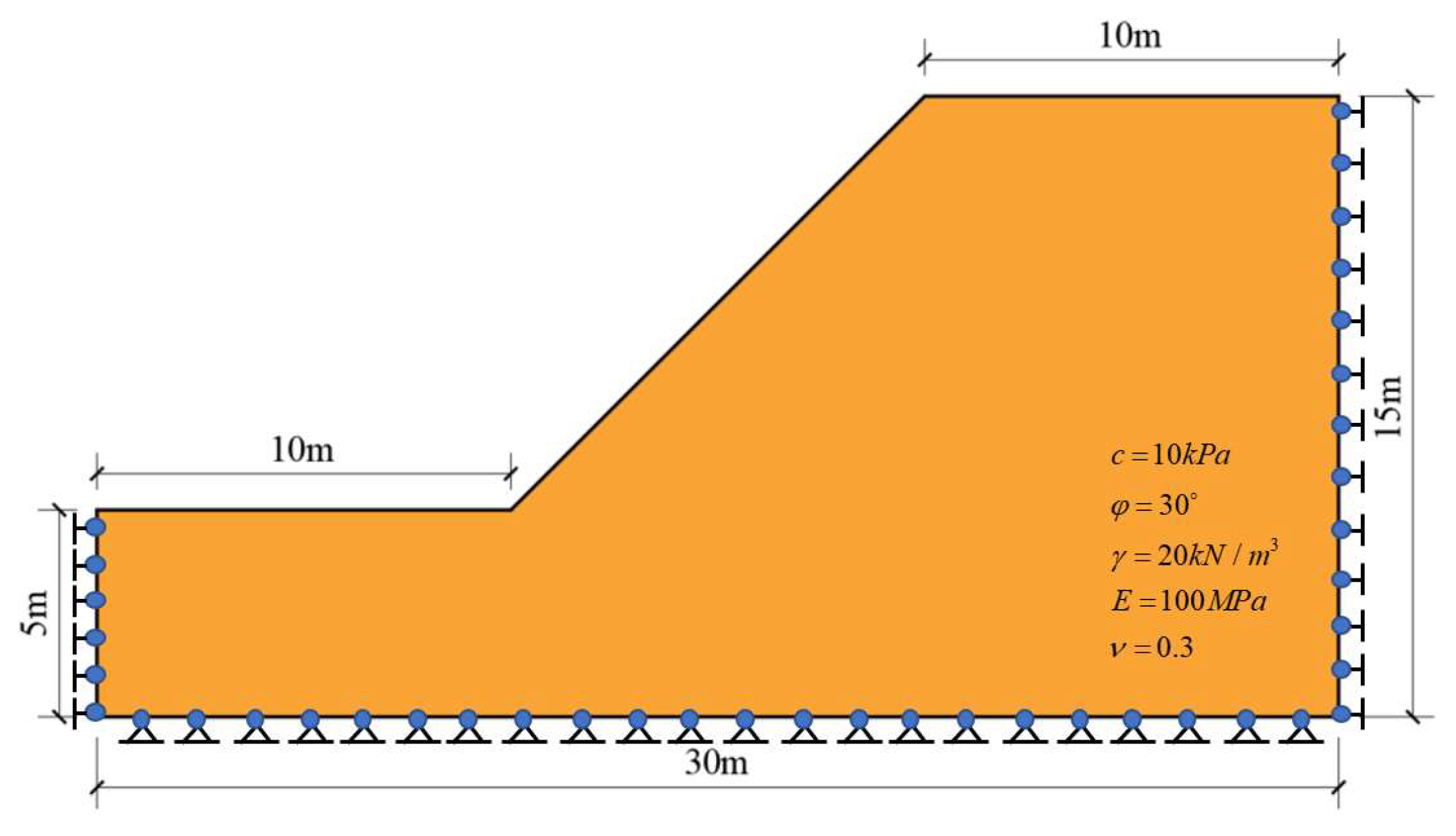
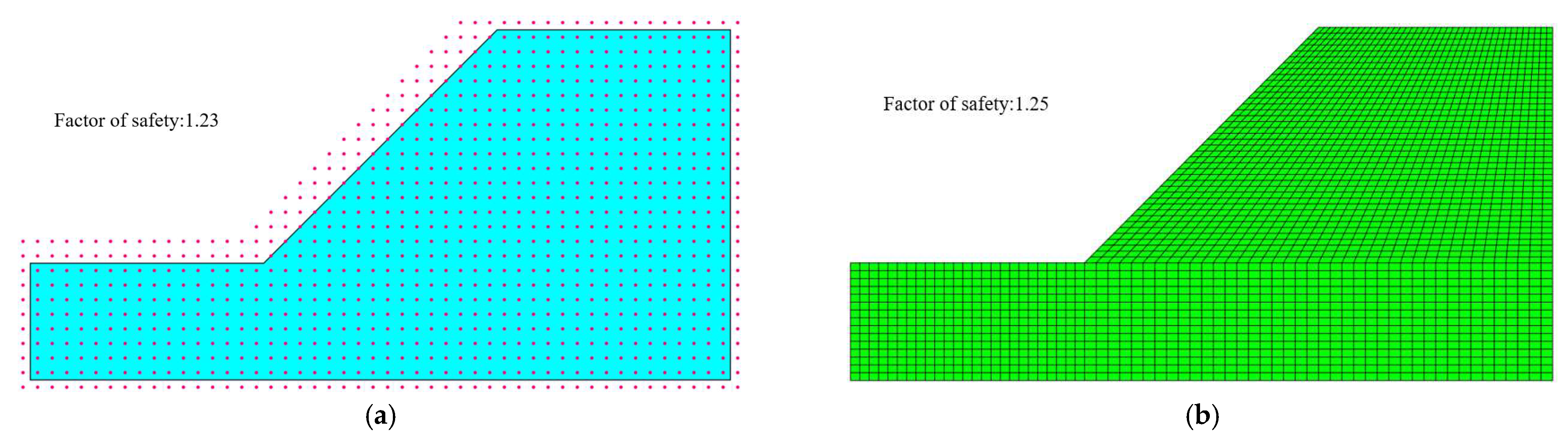
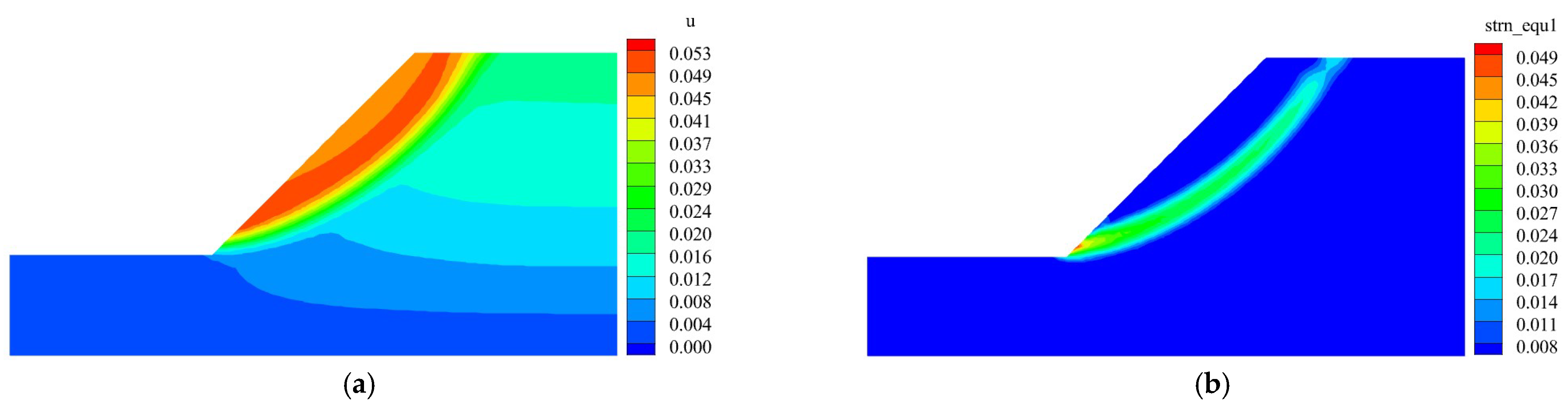
4.1. Slope Description and Deterministic Analysis

Figure 3 illustrates the geometric dimensions of the studied slope, which has a height of 15 m and a horizontal length of 10 m. The soil properties are as follows: elastic modulus $E=100 \mathrm{MPa}$, unit weight $\gamma =20{ \mathrm{kN}/\mathrm{m}}^3$, Poisson’s ratio $\nu =0.3$, cohesion $c=10 \mathrm{kPa}$, and internal friction angle $\phi ={30}^{\circ }$. The boundary conditions are defined such that the left and right vertical boundaries are fixed in the horizontal direction, while both horizontal and vertical displacements are constrained at the bottom boundary.

The Strength Reduction Method based on the Finite Element Method (FEM-SRM) is widely used for slope stability analysis due to its ability to handle complex boundary conditions and its capacity to provide comprehensive information on stress, displacement, and strain fields. Unlike traditional limit equilibrium methods (LEMs), FEM-SRM does not require prior assumptions regarding the interslice shear force distribution, making it more suitable for modeling realistic soil behavior under various loading and geological conditions. However, FEM-SRM has certain limitations. Its results are highly sensitive to mesh discretization and the choice of nonlinear solution algorithms. Cheng et al. [34] conducted an extensive comparison between two-dimensional LEM and FEM-SRM, showing that for simple homogeneous slopes, both methods yield similar results. Nevertheless, in the presence of weak interlayers or material heterogeneities, FEM-SRM’s accuracy becomes heavily dependent on the mesh quality and the nonlinear solver employed. When spatial variability in geotechnical parameters is considered—commonly modeled using Gaussian random fields—complex spatial patterns can emerge. Under highly heterogeneous conditions, slope configurations containing weak layers are likely to develop [35,36], significantly affecting the reliability of FEM-SRM outcomes.

To overcome the mesh dependency and enhance numerical performance, Zheng et al. [37] introduced the Meshless Numerical Manifold Method (MNMM), which integrates the Moving Least Squares (MLS) approximation into the Numerical Manifold Method (NMM) framework. MNMM can be regarded as a meshless Galerkin-type method within the NMM framework. It constructs the mathematical cover using the support domain of MLS-distributed nodes and defines weight functions based on MLS shape functions. As illustrated in Figure 4, the blue support domain of the black MLS node forms the mathematical cover, which is subsequently intersected by physical boundaries or material interfaces to form the physical cover (e.g., mathematical element M1 generates physical element P1 after intersection). The flexibility of MNMM lies in its ability to place mathematical nodes independently of the problem domain geometry, thus eliminating the requirement for mesh conformity or actual intersection with physical boundaries. Although background cells are still used to perform numerical integration—similar to the Element-Free Galerkin Method (EFGM)—MNMM separates the interpolation process from numerical integration via two independent systems: the mathematical cover and the physical cover. This decoupling enables a more natural representation of discontinuities in the solution field, improving both numerical accuracy and computational stability [38]. Compared to FEM, MNMM combines the advantages of MLS and NMM, offering greater flexibility and higher efficiency. It has been successfully applied in a variety of engineering problems, including fracture mechanics, seepage analysis, plate and shell structures, and slope stability analysis [37,38]. In slope stability modeling, MNMM is particularly advantageous because it is inherently independent of mesh discretization, thereby eliminating mesh-induced errors. This makes MNMM highly capable of accurately and reliably capturing the influence of spatial variability on slope stability, providing a robust and adaptive computational tool for analyzing slopes under complex geological conditions. For more detailed information on the MNMM framework, readers are referred to [38].

Given these advantageous numerical properties, this study employs MNMM for slope stability analysis. The F_s is computed based on an elastoplastic model and the Mohr-Coulomb yield criterion. To verify the accuracy of the MNMM results, a comparative analysis is conducted using the commercial finite element software Abaqus (latest v. 2025). Figure 5 presents the MNMM mathematical cover layout alongside the Abaqus mesh configuration. The MNMM model consists of 955 mathematical nodes, whereas Abaqus employs 2696 finite element nodes. The computed factors of safety from MNMM and Abaqus are 1.23 and 1.25, respectively, demonstrating a high degree of agreement. This close correlation validates the accuracy and reliability of MNMM in slope stability computations.

Figure 6 and Figure 7 present the displacement contour plots and equivalent plastic strain (PEEQ) contour plots obtained from MNMM and Abaqus, respectively. As shown in the displacement contour plots, both methods capture a well-defined sliding mass within the slope, with the maximum displacement concentrated near the slope surface, which aligns with typical slope failure characteristics. The PEEQ contour plots reveal a continuous plastic failure zone extending from the toe to the crest of the slope, indicating that the slope is in a critical stability state. The close agreement between the results obtained from MNMM and Abaqus further validates that the factor of safety computed by MNMM effectively reflects the critical failure condition of the slope. This confirms the accuracy and reliability of MNMM in slope stability analysis, demonstrating its potential as a robust numerical method for geotechnical engineering applications.

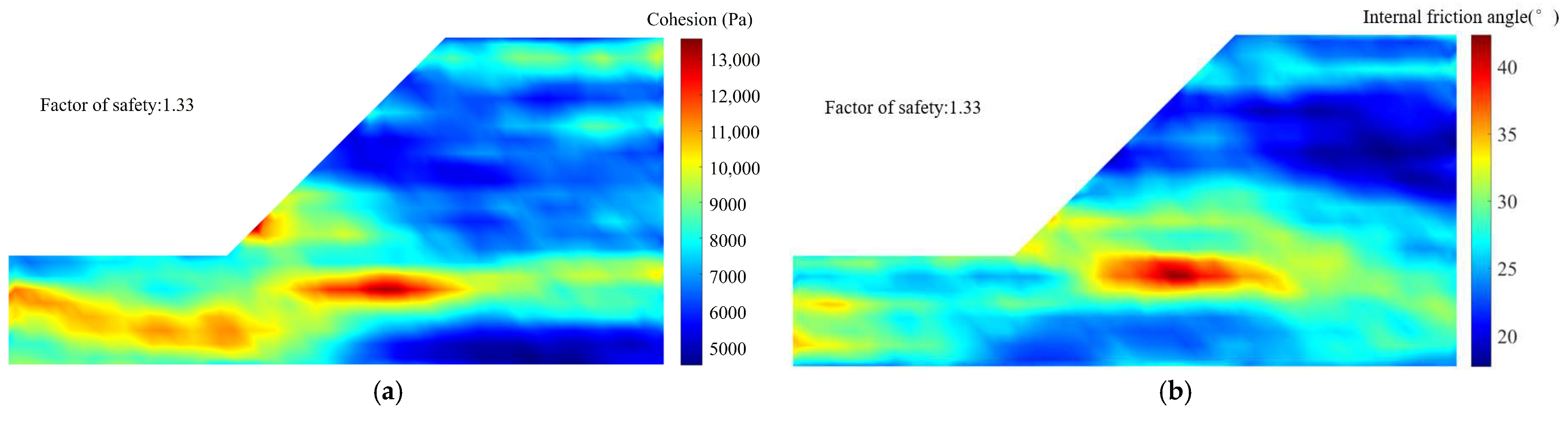
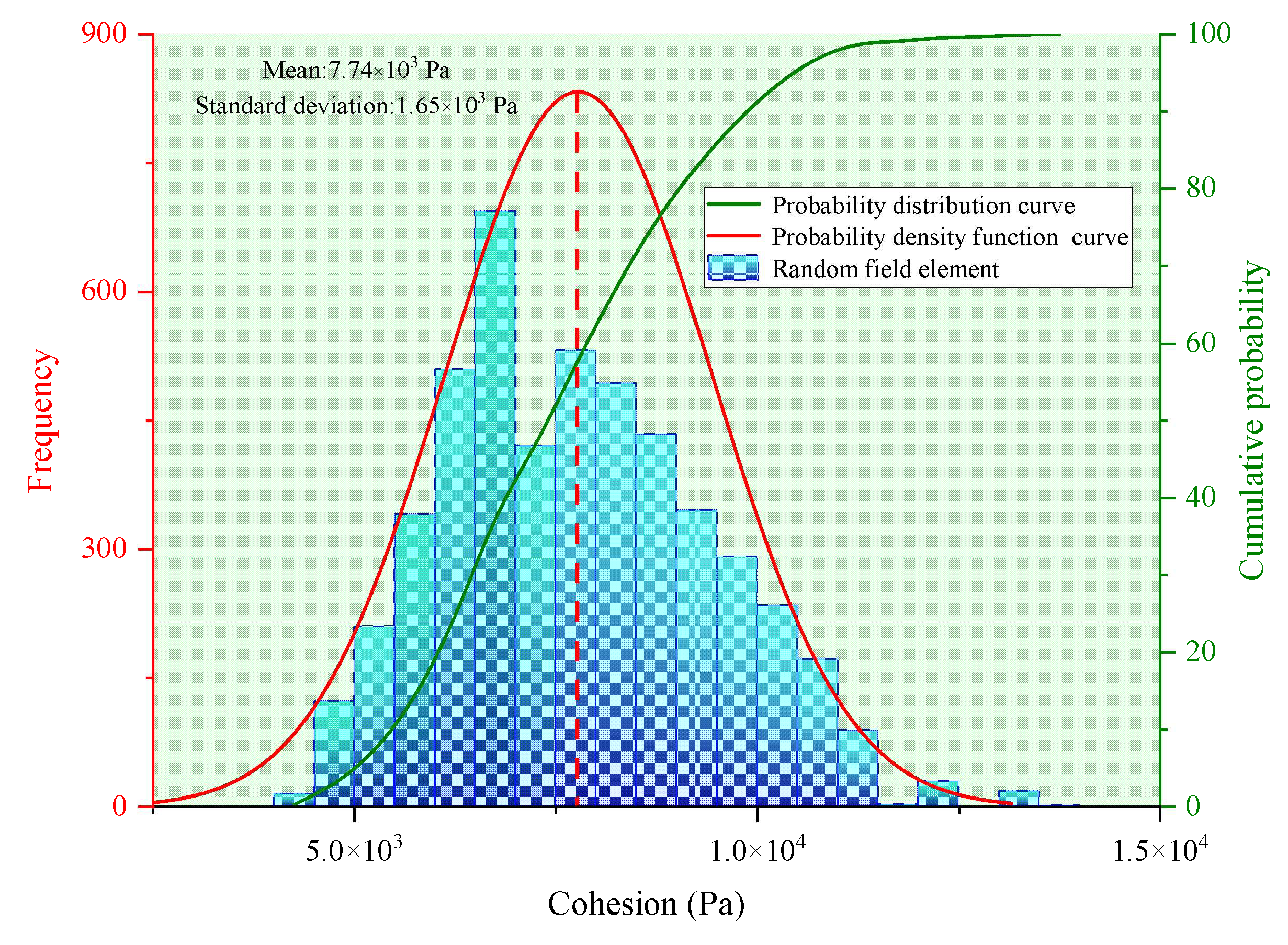
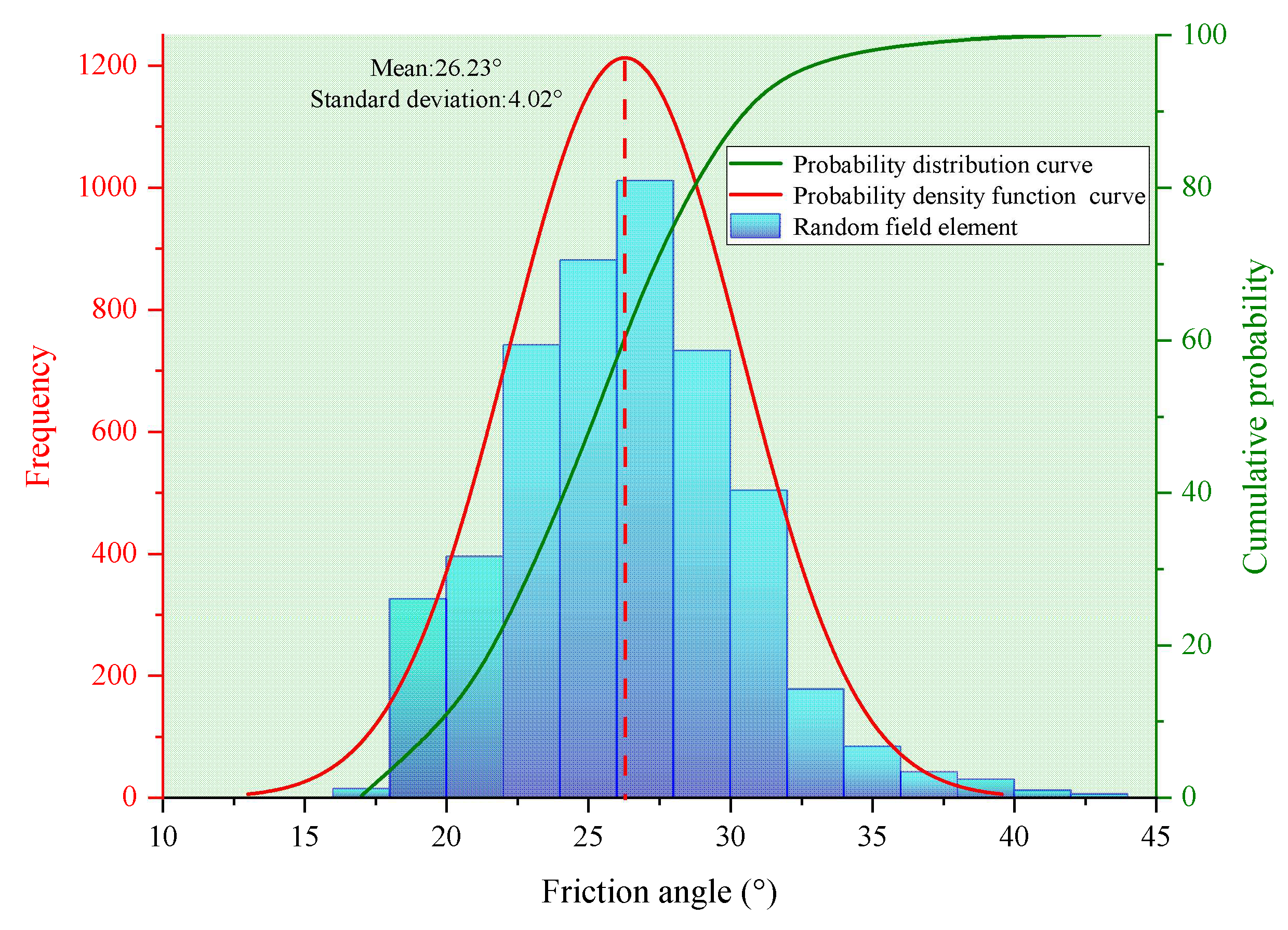
4.2. Random Field Distribution of Spatially Variable Slopes

During the formation of geotechnical materials, their micro- and macro-scale properties are often influenced by multiple independent and stochastic factors, such as diagenetic environment, sedimentary conditions, and post-depositional weathering. The complex spatial and temporal interactions of these factors result in significant spatial variability in geotechnical parameters. According to the central limit theorem, the combined effect of multiple independent random variables tends to follow a normal distribution. Consequently, key mechanical parameters of geomaterials, such as cohesion and internal friction angle, are typically modeled using Gaussian random fields, providing a theoretical foundation for applying random field methods in slope stability analysis.

In this study, a random field slope model considering spatial variability was established based on MNMM. The fluctuation ranges of the random field were set as ${\delta }_h=40 \mathrm{m}$, ${\delta }_v=4 \mathrm{m}$, and Gaussian random field parameters listed in

Table 1. Log-normal random field statistics for single-layer slope.

Soil Parameters	Mean	Coefficient of Variation	Distribution	Cross-Correlation Coefficient
c	10 kPa	0.3	Logarithmic	−0.5
φ	30°	0.2	Logarithmic

were used for modeling. The random field was discretized using the Cholesky decomposition method to ensure the reasonableness of spatial variability and numerical stability. Regarding the probability distribution of random variables, both c and φ were assumed to follow a lognormal distribution, with coefficients of variation (COV) of 0.3 and 0.2, respectively. Previous studies have shown that c and φ generally exhibit a weak negative correlation, meaning that variations in one parameter tend to influence the other. The correlation coefficient between c and φ typically ranges from −0.7 to −0.24 [39]. In this study, a correlation coefficient of −0.5 was adopted to represent a moderate negative correlation between the two parameters.

Figure 8 presents the typical random field distributions of c and φ generated based on the parameters in Table 1. Since c and φ are statistically independent random variables, their spatial distributions do not exhibit complete consistency. However, due to their inherent cross-correlation, a certain degree of local distributional correlation can still be observed. Figure 8a illustrates the spatial distribution of c within the slope, with a color scale representing its spatial variation, ranging approximately from 5000 Pa to 13,000 Pa. Red areas indicate higher cohesion values, while blue areas represent lower values. The figure demonstrates that cohesion exhibits localized high and low values with stochastic fluctuations, which is a characteristic feature of spatial variability captured by the random field method. Since a correlation length was predefined during random field generation, cohesion values exhibit strong local correlation within a certain spatial range, but this correlation rapidly diminishes beyond that range. Consequently, clusters of similar colors are observed in certain regions, indicating the presence of local spatial correlation in cohesion.

Figure 8b presents the spatial distribution of φ, using the same color scale as in Figure 8a, with values ranging from approximately 20° to 40°. Similar to cohesion, φ also exhibits localized high and low values with stochastic variations and maintains strong correlation within a defined spatial range, which decays rapidly beyond that range. Due to the negative correlation between c and φ, regions with higher cohesion values tend to have lower internal friction angles (relative to their respective mean values) and vice versa. This phenomenon influences the spatial distribution of shear strength. Moreover, if both c and φ simultaneously reach extreme high or low values at a specific location, it may result in local “over-strengthened” or “over-weakened” zones, where shear strength is abnormally high or low. The presence of a negative correlation reduces the probability of simultaneous extreme values, thereby affecting the overall stability distribution and failure risk of the slope.

Figure 9 and Figure 10 further display the statistical characteristics of the probability distributions of c and φ in the generated random field. Figure 9 shows the probability distribution of cohesion, where the blue histogram represents the distribution of cohesion values among all elements in the random field. The x-axis denotes cohesion values (Pa), while the left y-axis represents frequency. The histogram exhibits a bell-shaped distribution, characterized by a peak in the middle and lower frequencies on both sides, which closely aligns with the normal probability density function (PDF) shown by the red curve. This agreement suggests that the sample-level cohesion distribution is consistent with the Gaussian assumption. The red curve represents the fitted normal PDF, providing a smoothed idealized representation of the histogram. Additionally, the green curve represents the cumulative distribution function, which describes the cumulative probability of cohesion values being less than or equal to a specific value, with the corresponding scale indicated on the right y-axis (percentage). The dashed line marks the mean cohesion value of 7.74 × 10³ Pa, representing the central tendency of the distribution. The standard deviation is 1.65 × 10³ Pa, indicating the degree of dispersion in cohesion values. A larger standard deviation corresponds to greater spatial fluctuations, further reflecting the extent of variation around the mean.

Figure 10 presents the probability distribution of the internal friction angle, with a mean of 26.23° and a standard deviation of 4.02°, similarly characterizing the degree of dispersion. A larger standard deviation implies significant spatial variability in φ, analogous to cohesion, and its distribution characteristics are influenced by the random field parameters. By utilizing experimental data and the documented literature, key parameters such as the mean and variance of c and φ can be statistically determined. These parameters are then used to construct Gaussian random fields for subsequent numerical simulations and reliability analysis. This probabilistic approach provides a theoretical basis for modeling the spatial variability of geotechnical parameters, enabling a more accurate representation of the uncertainties in soil mechanical properties within complex geological environments.

The random field model provides a more realistic approach for slope stability analysis. Traditional deterministic analysis assumes that soil parameters remain constant across the entire slope domain, whereas the random field method allows c and φ at each computational element to be sampled from a Gaussian random field. This approach better captures the spatial variability of soil mechanical properties. In this study, the Fs obtained using the random field method is 1.33, slightly higher than the deterministic analysis result of 1.23. This difference suggests that incorporating spatial variability in geotechnical parameters alters the slope stability assessment, which may be attributed to the following factors: (1) In the spatial variability model, certain regions may exhibit locally higher shear strength, enhancing overall slope stability. (2) Due to the negative correlation between c and φ, the random field method effectively reduces the likelihood of extreme weak zones, thereby mitigating localized instability risks. (3) The presence of a random field may shift the critical sliding surface, making it more likely to pass through weaker regions, thus affecting the computed Fs.

The application of the random field method in slope stability analysis is of significant importance. It not only provides a more realistic representation of the spatial variability of geotechnical parameters but also offers a more reliable quantitative approach for stability assessment and risk prediction. Therefore, incorporating the random field method into practical engineering applications enables a more accurate evaluation of slope failure risks, providing a scientific basis for engineering design.

4.3. Surrogate Model-Based Factor of Safety Prediction Analysis

In the training process of machine learning algorithms, Bayesian optimization (BO) is an efficient hyperparameter tuning method, particularly suitable for computationally expensive tasks. Unlike traditional grid search and random search methods, BO strategically explores the hyperparameter search space by prioritizing regions with the most informative configurations, thereby significantly improving optimization efficiency. A key component of BO is the Gaussian process (GP), which helps model the distribution of the objective function. During optimization, the GP dynamically updates prior information based on observed data, enabling continuous refinement of hyperparameter selection. Compared to conventional methods, BO requires fewer iterations, reduces the risk of overfitting and local minima, and ensures a more robust and fair evaluation of the model. In this study, BO is employed to optimize the hyperparameters of the CNN model, with the objective of minimizing the MSE on the validation set. The optimized hyperparameters include the initial learning rate, regularization coefficient, and dropout rate. The search intervals, commonly used default values, and the final optimized values are summarized in

Table 2. Hyperparameters of CNN optimized by Bayesian optimization.

Hyperparameters	Optimization Interval	Default Value	Optimal Hyperparameters
Initialize learning rate	[0.0001, 0.01]	0.001	4.15 × 10−4
Regularization coefficient	[1 × 10−8, 1 × 10−2]	0.0001	6.73 × 10−6
Dropout rate	[0.2, 0.6]	0.5	0.315

. Specifically, the initial learning rate was searched within the range of [0.0001, 0.01], with a commonly adopted default value of 0.001. The optimization process identified an optimal value of 4.15 × 10⁻⁴. For the regularization coefficient, the search interval was set to [1 × 10⁻⁸, 1 × 10⁻²], with a default value of 1 × 10⁻⁴, and the optimal value determined was 6.73 × 10⁻⁶. The dropout rate was explored in the range [0.2, 0.6], with a typical default of 0.5, while the final optimized value was 0.315.

These results reveal that the optimal hyperparameters deviate significantly from their default settings, suggesting that relying on default values would have led to suboptimal model performance. The wide search ranges and the sensitivity of the model to these parameters highlight the importance of conducting thorough hyperparameter optimization. This process is essential to enhance model generalization and training stability, thereby ensuring more accurate and reliable predictions in geotechnical engineering applications.

Figure 11 illustrates the training process of the CNN model, depicting the variation in MSE with the number of iterations for both the training and validation datasets. It can be observed that, after approximately 20 iterations, the loss values for both datasets decline sharply and subsequently stabilize. Throughout the training process, the validation loss gradually decreases without exhibiting an increasing trend, indicating that Bayesian optimization effectively prevents overfitting. Additionally, the validation loss remains higher than the training loss and exhibits some degree of fluctuation. This discrepancy arises because the validation set contains previously unseen data, which inherently leads to a slightly higher loss and occasional variations. As training progresses, both the training and validation loss values stabilize and converge, demonstrating that the model, with appropriate regularization techniques, achieves a balanced trade-off between learning from the training data and generalizing to unseen samples. This convergence confirms the effectiveness of the adopted optimization strategy in enhancing the model’s generalization performance.

To evaluate the performance of the surrogate model in predicting the Fs for slopes with spatial variability, the randomly generated distributions of cohesion and internal friction angle (Figure 8) were used as input, while the Fs values computed from the MNMM-based approach served as the regression target. Figure 12 presents a comparison between the predicted and reference Fs values on the test set, illustrating both the mean and standard deviation variations across different test samples. The results show that the predicted mean and standard deviation closely align with the reference values, demonstrating that the surrogate model effectively captures the statistical characteristics of Fs and accurately reflects the influence of spatial variability. Furthermore, to quantitatively assess the prediction accuracy, the RMSE was calculated, yielding a value of 0.035. This result confirms that the surrogate model achieves high predictive accuracy and can serve as a reliable substitute for numerical simulations, enabling efficient evaluation of complex slope systems.

5. Conclusions

This paper proposes a surrogate model-based approach to accurately predict the Fs for slopes while accounting for spatial variability in geotechnical parameters. The effectiveness of the proposed method has been validated, leading to the following conclusions:

(1)

A Gaussian random field model was established for c and φ, and the results confirm that their distributions align well with statistical assumptions. This model effectively captures the spatial uncertainty and correlation of geotechnical parameters, providing a theoretical basis for slope stability analysis.

(2)

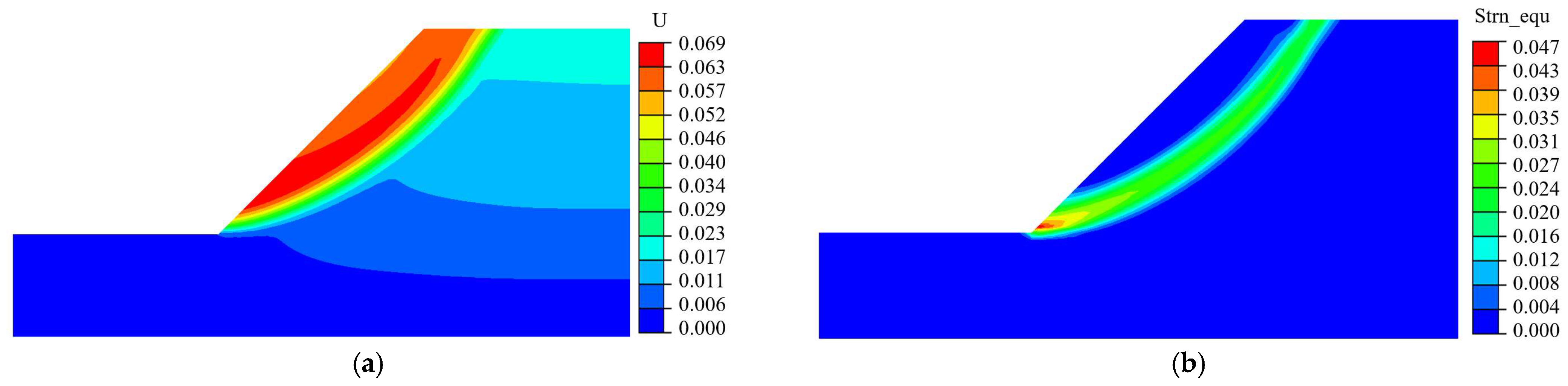
Compared with deterministic analysis, the random field approach yields Fs values that better reflect the uncertainty in geotechnical parameters. Spatial variability can induce localized strength reductions, potentially affecting overall stability, highlighting the necessity of incorporating random field modeling in slope stability assessment.

(3)

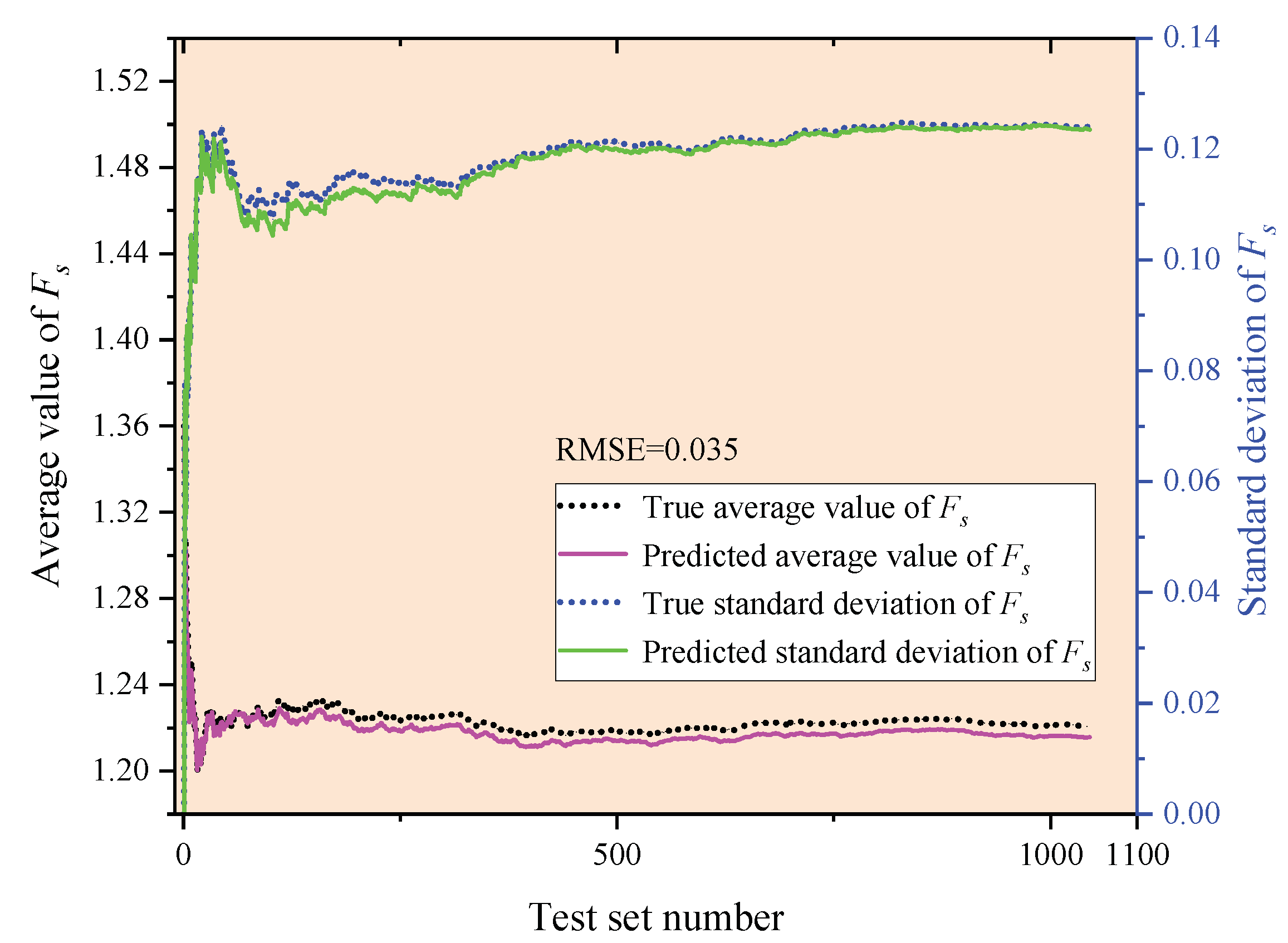
The proposed surrogate model demonstrates excellent performance in predicting Fs, with predicted values closely matching the ground truth. The model achieves an RMSE of just 0.035, indicating its capability to reliably replace complex numerical simulations for efficient evaluation of slope stability under spatial variability.

References

1. Jiang, S.; Huang, J.; Griffiths, D.V.; Deng, Z. Advances in reliability and risk analyses of slopes in spatially variable soils: A state-of-the-art review. Comput. Geotech. 2022, 141, 104498. [Google Scholar] [CrossRef]
2. El-Ramly, H.; Morgenstern, N.R.; Cruden, D.M. Probabilistic slope stability analysis for practice. Can. Geotech. J. 2002, 39, 665–683. [Google Scholar] [CrossRef]
3. Phoon, K.K.; Kulhawy, F.H. Characterization of geotechnical variability. Can. Geotech. J. 1999, 36, 612–624. [Google Scholar] [CrossRef]
4. Baecher, G.B.; Christian, J.T. Reliability and Statistics in Geotechnical Engineering; John Wiley and Sons: New York, NY, USA, 2003. [Google Scholar]
5. Bourne-Webb, P.J. Book review: Risk assessment in geotechnical engineering. Geotechnique 2011, 61, 186. [Google Scholar] [CrossRef]
6. Cho, S.E. Effects of spatial variability of soil properties on slope stability. Eng. Geol. 2007, 92, 97–109. [Google Scholar] [CrossRef]
7. Cho, S.E. Probabilistic stability analysis of rainfall-induced landslides considering spatial variability of permeability. Eng. Geol. 2014, 171, 11–20. [Google Scholar] [CrossRef]
8. Wang, L.; Wu, C.Z.; Li, Y.Q.; Liu, H.L.; Zhang, W.G.; Chen, X. Probabilistic Risk Assessment of unsaturated Slope Failure Considering Spatial Variability of Hydraulic Parameters. KSCE J. Civ. Eng. 2019, 23, 5032–5040. [Google Scholar] [CrossRef]
9. Zienkiewicz, O.C.; Humpheson, C.; Lewis, R.W. Associated and non-associated visco-plasticity and plasticity in soil mechanics. Geotechnique 1975, 25, 671–689. [Google Scholar] [CrossRef]
10. Zheng, H.; Liu, D.F.; Li, C.G. Slope stability analysis based on elasto-plastic finite element method. Int. J. Numer. Methods Eng. 2005, 64, 1871–1888. [Google Scholar] [CrossRef]
11. Ugai, K. A Method of Calculation of Total Safety Factor of Slope by Elasto-Plastic FEM. Soils Found. 1989, 29, 190–195. [Google Scholar] [CrossRef]
12. Matsui, T.; San, K. Finite Element Slope Stability Analysis by Shear Strength Reduction Technique. Soils Found. 1992, 32, 59–70. [Google Scholar] [CrossRef]
13. Griffiths, D.V.; Lane, P.A. Slope stability analysis by finite elements. Geotechnique 1999, 49, 387–403. [Google Scholar] [CrossRef]
14. Stead, D.; Eberhardt, E.; Coggan, J.S. Developments in the characterization of complex rock slope deformation and failure using numerical modelling techniques. Eng. Geol. 2006, 83, 217–235. [Google Scholar] [CrossRef]
15. Gravanis, E.; Pantelidis, L.; Griffiths, D.V. An analytical solution in probabilistic rock slope stability assessment based on random fields. Int. J. Rock Mech. Min. Sci. 2014, 71, 19–24. [Google Scholar] [CrossRef]
16. Schweiger, H.F.; Peschl, G.M. Reliability analysis in geotechnics with the random set finite element method. Comput. Geotech. 2005, 32, 422–435. [Google Scholar] [CrossRef]
17. Wu, C.; Wang, Z.Z.; Goh, S.H.; Zhang, W. Comparing 2D and 3D slope stability in spatially variable soils using random finite-element method. Comput. Geotech. 2024, 170, 106324. [Google Scholar] [CrossRef]
18. Su, Y.; Luo, Z.; Zhang, P. Active searching algorithm for slope stability reliability based on Kriging model. Chin. J. Geotech. Eng. 2013, 35, 1863–1869. [Google Scholar]
19. Zhang, T.; Zeng, P.; Li, T. System reliability analyses of slopes based on active-learning radial basis function. Rock Soil Mech. 2020, 41, 3098–3108. [Google Scholar]
20. Karniadakis, G.E.; Kevrekidis, I.G.; Lu, L.; Perdikaris, P.; Wang, S.; Yang, L. Physics-informed machine learning. Nat. Rev. Phys. 2021, 3, 422–440. [Google Scholar] [CrossRef]
21. Hu, H.; Qi, L.; Chao, X. Physics-informed neural networks (pinn) for computational solid mechanics: Numerical frameworks and applications. Thin-Walled Struct. 2024, 205, 112495. [Google Scholar] [CrossRef]
22. Griffiths, D.V.; Fenton, G.A. Probabilistic slope stability analysis by finite elements. J. Geotech. Geoenvironmental Eng. 2004, 130, 507–518. [Google Scholar] [CrossRef]
23. Huang, J.S.; Griffiths, D.V.; Fenton, G.A. System Reliability of Slopes by RFEM. Soils Found. 2010, 50, 343–353. [Google Scholar] [CrossRef]
24. Li, D.Q.; Jiang, S.H.; Cao, Z.J.; Zhou, W.; Zhou, C.B.; Zhang, L.M. A multiple response-surface method for slope reliability analysis considering spatial variability of soil properties. Eng. Geol. 2015, 187, 60–72. [Google Scholar] [CrossRef]
25. Phoon, K. Role of reliability calculations in geotechnical design. Georisk Assess. Manag. Risk Eng. Syst. Geohazards 2017, 11, 4–21. [Google Scholar] [CrossRef]
26. Wang, Z.Z.; Goh, S.H. Novel approach to efficient slope reliability analysis in spatially variable soils. Eng. Geol. 2021, 281, 105989. [Google Scholar] [CrossRef]
27. Griffiths, D.V.; Huang, J.S.; Fenton, G.A. Influence of Spatial Variability on Slope Reliability Using 2-D Random Fields. J. Geotech. Geoenvironmental Eng. 2009, 135, 1367–1378. [Google Scholar] [CrossRef]
28. Ditlevsen, O.; Madsen, H.O. Structural Reliability Methods; Technical University of Denmark: Lyngby, Denmark, 1996. [Google Scholar]
29. Lyu, H.; Yin, Z.; Hicher, P.; Laouafa, F. Incorporating mitigation strategies in machine learning for landslide susceptibility prediction. Geosci. Front. 2024, 15, 101869. [Google Scholar] [CrossRef]
30. Lyu, S.; Wang, L.; Zhou, Z. Improving generalization of deep neural networks by leveraging margin distribution. Neural Netw. 2022, 151, 48–60. [Google Scholar] [CrossRef]
31. Chen, Z.; Liu, F. An implicit thermo-mechanical coupling model for heat conduction and thermal cracking in brittle materials. Comput. Geotech. 2024, 166, 106033. [Google Scholar] [CrossRef]
32. Guo, H.; Yin, Z.Y. A novel physics-informed deep learning strategy with local time-updating discrete scheme for multi-dimensional forward and inverse consolidation problems. Comput. Methods Appl. Mech. Eng. 2024, 421, 116819. [Google Scholar] [CrossRef]
33. Li, K.; Yin, Z.; Zhang, N.; Li, J. A PINN-based modelling approach for hydromechanical behaviour of unsaturated expansive soils. Comput. Geotech. 2024, 169, 106174. [Google Scholar] [CrossRef]
34. Cheng, Y.M.; Lansivaara, T.; Wei, W.B. Two-dimensional slope stability analysis by limit equilibrium and strength reduction methods. Comput. Geotech. 2007, 34, 137–150. [Google Scholar] [CrossRef]
35. Chen, F.Y.; Wang, L.; Zhang, W.G. Reliability assessment on stability of tunnelling perpendicularly beneath an existing tunnel considering spatial variabilities of rock mass properties. Tunn. Undergr. Space Technol. 2019, 88, 276–289. [Google Scholar] [CrossRef]
36. Zheng, Y.; Chen, C.; Liu, T.; Xia, K.; Sun, C.; Chen, L. Analysis of a retrogressive landslide with double sliding surfaces: A case study. Environ. Earth Sci. 2020, 79, 21. [Google Scholar] [CrossRef]
37. Zheng, H.; Liu, F.; Li, C. The MLS-based numerical manifold method with applications to crack analysis. Int. J. Fract. 2014, 190, 147–166. [Google Scholar] [CrossRef]
38. Cao, X.; Lin, S.; Liang, Z.; Guo, H.; Zheng, H. Meshless numerical manifold method with novel subspace tracking and CSS locating techniques for slope stability analysis. Comput. Geotech. 2024, 166, 106025. [Google Scholar] [CrossRef]
39. Cherubini, C. Data and Consideration on the Variability of Geotechnical Properties of Soils. In Proceedings of the International Conference on Safety and Reliability, ESREL 1997, Lisbon, Portugal, 17–20 June 1997; pp. 1583–1591. [Google Scholar]
Figure 1. Schematic diagram of CNN convolutional layer and pooling layer for slope stability analysis. (a) CNN input layers that make up a digital image; (b) CNN input layers that constitute the c-φ image for slope stability analysis; (c) CNN convolution layer and pooling layer calculation principle.
Mathematics 13 01604 g001
Figure 2. CNN-based surrogate model architecture.
Mathematics 13 01604 g002
Figure 3. Geometry of single-layer c-φ slope.
Mathematics 13 01604 g003
Figure 4. The process of generating physical slices from MNMM math nodes and typical math slices (black boxes and blue dots represent math slices and corresponding math nodes, respectively).
Mathematics 13 01604 g004
Figure 5. MNMM covering system and FEM meshing. (a) MNMM covering system; (b) FEM meshing.
Mathematics 13 01604 g005
Figure 6. Displacement and strain contours obtained from MNMM computation. (a) Displacement contour. (b) Equivalent plastic strain contour.
Mathematics 13 01604 g006
Figure 7. Displacement and strain contours obtained from FEM computation. (a) Displacement contour. (b) Equivalent plastic strain contour.
Mathematics 13 01604 g007
Figure 8. Typical realizations of c and φ random fields. (a) Realization of c random field. (b) Realization of φ random field.
Mathematics 13 01604 g008
Figure 9. Probability distribution of c random field.
Mathematics 13 01604 g009
Figure 10. Probability distribution of φ random field.
Mathematics 13 01604 g010
Figure 11. Training process of the CNN model.
Mathematics 13 01604 g011
Figure 12. Comparison of mean and standard deviation of true and predicted Fs in the test set.
Mathematics 13 01604 g012