Enhancing Predictive Accuracy in Medical Data Through Oversampling and Interpolation Techniques

Abstract

Class imbalance is a major challenge in supervised classification, often leading to biased predictions and limited generalization. This issue is particularly pronounced in medical diagnostics, where datasets typically contain far more negative than positive cases. In this study, we compare two oversampling strategies: the Synthetic Minority Oversampling Technique (SMOTE) and the Conditional Tabular Generative Adversarial Network (ctGAN). Using the benchmark Pima Indians Diabetes dataset, we generated balanced datasets through both methods and trained a multilayer perceptron classifier. Performance was evaluated with accuracy, precision, sensitivity, and F1 Score. The results show that both SMOTE and ctGAN improve classification on imbalanced data, with SMOTE consistently achieving superior sensitivity and F1 Score. These findings highlight the importance of selecting appropriate augmentation strategies to enhance the reliability and clinical usefulness of machine learning models in medical diagnostics.

1. Introduction

With the increasing adoption of artificial intelligence (AI) and machine learning (ML) in fields such as medical diagnostics, finance, and industry, ensuring the quality and representativeness of data has become a critical challenge. A particularly common issue is the class imbalance problem, which arises when one class is significantly overrepresented relative to others. In supervised classification, this leads algorithms to favor the majority class, often yielding deceptively high accuracy while failing to generalize to minority cases [1,2,3]. The result is biased predictions, limited sensitivity, and incomplete representation of minority class patterns.

To mitigate these issues, a variety of strategies have been proposed, including resampling (oversampling or undersampling) [4], cost-sensitive learning [5], ensemble methods [6], and data augmentation [7,8,9]. Oversampling expands the minority class by creating synthetic samples, with the Synthetic Minority Oversampling Technique (SMOTE) [10,11,12] being the most widely used approach. It interpolates between neighboring minority samples to generate new instances, improving representation but risking overfitting when diversity is low. Recent variants of SMOTE, such as DeepSMOTE [13], combine deep learning with SMOTE for enhanced performance. In contrast, undersampling reduces the majority class, which can alleviate imbalance but may also discard valuable information.

Data augmentation offers an alternative by generating new instances that capture richer variability of the minority class. Generative models, in particular Generative Adversarial Networks (GANs) [14,15,16], learn the underlying data distribution and create realistic yet novel samples. Their recent variants, such as the Conditional Tabular GAN (ctGAN) [17,18], extend this framework to tabular data, allowing conditional generation based on class labels or feature constraints.

Recent advances in generative modeling have expanded beyond traditional GAN architectures, with several promising alternatives emerging for tabular data generation. DDPMs have shown remarkable success in generating high-quality synthetic data by learning to reverse a gradual noise corruption process, offering potential advantages in training stability and sample diversity compared to adversarial training [19]. In particular, Liu et al. demonstrate that DDPM-based approaches can achieve superior performance in small-sample regimes, where models with attention mechanisms often degrade significantly [19]. Variational autoencoders (VAEs) and their conditional variants provide another alternative, learning latent representations that enable controlled generation [20]. Additionally, flow-based models and autoregressive approaches have been adapted for tabular data, each with distinct trade-offs in terms of training complexity, sample quality, and computational requirements, while this study focuses on ctGAN as a representative GAN-based approach for tabular data—owing to its demonstrated effectiveness in medical data augmentation and established comparability with SMOTE in the prior literature. The choice to compare SMOTE and ctGAN directly reflects our aim to contrast a classical, interpretable interpolation method with a modern generative adversarial approach specifically designed for tabular medical data, thereby providing practitioners with evidence-based guidance for the most commonly employed techniques in medical machine learning.

The relevance of these techniques is especially pronounced in medical diagnostics, where datasets typically contain more negative (healthy) than positive (disease) cases [21,22,23,24]. This imbalance limits the clinical utility of ML models, reducing their ability to identify critical cases. Approaches such as oversampling, ensemble learning, and GAN-based augmentation have been applied in this context [25,26,27,28,29,30,31], but systematic comparisons remain limited.

In this work, we present a comparative study of two oversampling strategies for medical tabular data: the well-established SMOTE and the more recent ctGAN. Our objective is to evaluate which method generates higher-quality synthetic samples—better capturing the minority class distribution—and improves supervised classification performance.

Rather than proposing a new oversampling algorithm, this work presents a structured and reproducible comparative study of two widely used augmentation approaches –SMOTE and ctGAN– applied to a clinical prediction task. The contribution of the manuscript lies in the systematic evaluation framework, which integrates; consistent preprocessing and augmentation workflows; distributional similarity metrics; cross-validated classifier performance; and, statistical significance testing. By consolidating these assessment criteria within a unified experimental setting, the study provides a transparent comparison of how interpolation-based and generative augmentation behave under the same methodological constraints.

While several studies have compared SMOTE and GAN-based methods for class imbalance [29,30], our work differentiates itself through: a comprehensive multi-metric validation framework combining visual (KDE plots) and quantitative (Kolmogorov–Smirnov, Wasserstein, Jensen–Shannon, Anderson–Darling) assessments to rigorously evaluate distributional fidelity; explicit analysis of how augmentation affects minority class representation through class-stratified feature distributions; detailed computational complexity analysis comparing deterministic interpolation versus adversarial training; and critical discussion of clinical validation challenges, including the distinction between statistical variability and clinically meaningful diversity. Unlike prior work that primarily focuses on classification performance, we provide a deeper understanding of how each method preserves or distorts the underlying data distribution, which is crucial for medical applications where distributional fidelity directly impacts model trustworthiness and clinical interpretability.

To this end, we analyze the benchmark Pima Indians Diabetes dataset, a widely studied binary classification problem involving Indian women aged 21 years and older [32,33].

The remainder of this paper is organized as follows. Section 2 describes the dataset, methodology, and experimental setup. Section 3 presents the results and discussion. Finally, Section 4 concludes the paper and outlines future research directions.

2. Materials and Methods

2.1. The Binary Classification Dataset

The binary classification dataset (dataset available at URL https://www.kaggle.com/datasets/uciml/pima-indians-diabetes-database/data (accessed on 12 December 2025). Code available at https://github.com/elMaxPain/files/blob/master/SMOTE_v_GAN_Paper_2.ipynb (accessed on 12 December 2025)) relates to diabetes mellitus diagnosis in Indian women aged 21 and older. This dataset has been widely studied in supervised machine learning classification tasks [32,34]. As shown in

Table 1. Characteristics of the Pima Indians Diabetes dataset. The table summarizes the dimensionality and structure of the dataset used throughout this study, including the number of predictive features (eight clinical and physiological variables), the number of output classes (diabetic vs. non-diabetic), the type of prediction target (binary), and the total number of available instances (768 patient records). These characteristics define the baseline data distribution on which all preprocessing and augmentation procedures were applied.

Dataset	Number of Features	Number of Classes	Output Attributes	Number of Instances
Pima Indians Diabetes	8	2	1	768

, the Pima Indians Diabetes dataset comprises 768 instances characterized by 8 predictive features and one predicted feature. All the predictive features are numerical values that represent medical information and outcomes, such as the number of pregnancies, plasma glucose level, diastolic blood pressure, diabetes pedigree function, among others.

The predicted feature, or class attribute, refers to the outcome of the diabetes test; class value 1 is regarded as a positive test for diabetes, and class value 0 as a negative test.

Table 2. Distribution of instances by class in the Pima Indians Diabetes dataset. The table reports the absolute and relative frequencies of the two outcome classes: non-diabetic (class 0) and diabetic (class 1). The dataset exhibits a heavy imbalance, with 65.10% of instances belonging to the non-diabetic class and 34.90% to the diabetic class, a characteristic that motivates the use of oversampling and generative augmentation techniques in this study.

Class	Number of Instances	%
0	500	65.10
1	268	34.90
Total	768	100

show the distribution of the number of instances by class. Observe that the dataset exhibits a strong class imbalance, with the majority class representing over 65% of the total instances, almost twice the minority class.

2.2. The Synthetic Minority Oversampling Technique

The Synthetic Minority Oversampling Technique (SMOTE) [10,11,12] is a widely used method to address class imbalance through oversampling. SMOTE generates synthetic samples for the minority class, thereby mitigating the overfitting risk associated with random oversampling.

SMOTE works by identifying minority class instances that are close in the feature space and generating new samples along the line segments connecting them. For each minority instance, it selects the k nearest neighbors, randomly chooses one, and interpolates between the two. A user-defined parameter, known as the sampling ratio, determines the number of new samples to be generated per minority instance and the extent of interpolation.

By increasing the representation of the minority class and enriching its feature space, SMOTE helps to alleviate imbalance. However, if the generated samples are too similar to the originals, overfitting can occur. Variants of SMOTE integrate clustering or feature selection to further enhance diversity [35,36]. It is worth noting that SMOTE’s behavior in high-dimensional settings has been extensively studied [37], and comprehensive reviews have documented its progress and challenges over the years [38].

It is important to note that SMOTE’s linear interpolation approach generates synthetic samples along line segments connecting neighboring minority instances, which effectively constrains new samples to lie within the convex hull of existing minority cases, while this property can help preserve local structure and ensure that synthetic samples remain within the observed feature space, it assumes that minority cases form a relatively homogeneous group. However, in medical contexts such as diabetes diagnostics, minority cases may represent heterogeneous subgroups with distinct biomarker profiles and pathophysiological mechanisms. In such scenarios, convex hull-based interpolation may oversimplify the biological diversity and potentially blur clinically meaningful boundaries between atypical subtypes, such as early-onset diabetes with unusual glucose–insulin dynamics. Recent research has questioned the clinical validity of SMOTE in medical datasets, highlighting concerns about the representation of real-world patient variability [39]. Nevertheless, SMOTE remains valuable for its deterministic nature, computational efficiency, and ability to preserve statistical properties, particularly when minority class diversity is relatively constrained or when preserving a distribution closely aligned to the original is required.

SMOTE operates through three key steps: for each minority instance, it identifies k nearest neighbors from the minority class; it randomly selects one neighbor and generates synthetic samples via linear interpolation $x_{new}=x_i+\lambda (x_{nn}-x_i)$ where $\lambda \sim \mathcal{U}(0,1)$; and the process repeats until the target minority class size is reached [11].

Missing or zero-valued attributes were imputed using KNN with $k=3$. This approach was selected because; the dataset contains non-linear feature interactions that are not well-handled by mean/median imputation; and, medical variables in this dataset show local structure, such as clusters of similar BMI–glucose–insulin profiles. The choice of $k=3$ aligns with these findings and avoids the instability observed with smaller values ($k=1$ or $k=2$) or the oversmoothing that arises with larger neighborhoods.

Figure 1 illustrates the main steps of the SMOTE algorithm.

2.3. The Generative Adversarial Network

In recent years, Generative Adversarial Networks (GANs) [14,15,16] have emerged as a powerful deep learning approach for generative modeling, particularly in producing realistic images. In this work, we exploit their generative ability to augment datasets and mitigate class imbalance by generating new synthetic samples that approximate the underlying data distribution.

As illustrated in Figure 2, a GAN model consists of two components: a generator and a discriminator trained in an adversarial setting. The generator learns to map random noise into synthetic samples that resemble real data, while the discriminator learns to distinguish between real and synthetic samples. During training, the generator improves by attempting to fool the discriminator, and the discriminator improves by becoming more accurate in its classification task.

The discriminator is a neural network that receives input samples and outputs the probability of them being real. Its objective is to maximize accuracy in distinguishing genuine from synthetic data. Conversely, the generator transforms random noise into candidate samples with the goal of producing outputs that the discriminator cannot reliably separate from real data. The interplay between these two networks drives the generator to learn complex data distributions.

Through iterative training, the adversarial process enables GANs to produce high-quality synthetic data that closely resembles real samples, making them well suited for applications such as image generation, data augmentation, and—in our case—balancing imbalanced datasets.

2.4. The Conditional-Tabular Generative Adversarial Network

An adaptation of the GAN architecture, the conditional GAN [18], incorporates class labels or other conditioning variables into both the generator and discriminator, enabling controlled sample generation. For tabular data, ctGAN [17] extends this framework by integrating conditional information during training, allowing the model to target minority-class structure more accurately in imbalanced data.

Formally, ctGAN consists of a generator $G_{\gamma }$ that maps noise z and conditioning c to synthetic samples $x_{gen}=G_{\gamma }(z,c)$, and a discriminator $D_{\rho }$ that distinguishes real from generated data. Training optimizes the objective $V(D_{\rho },G_{\gamma })=V_{GAN}+KL(P\left(c\right)\Vert P_{syn}\left(c\right))$, where the conditional term promotes alignment between real and synthetic conditional distributions.

Because the KL divergence is mode-seeking, it may underrepresent rare clinical profiles; alternatives such as Jensen–Shannon divergence or entropy-based regularization could mitigate this limitation. In the present study, we retain the standard KL formulation to maintain consistency with established ctGAN implementations. At equilibrium, $G_{\gamma }$ produces condition-consistent samples that $D_{\rho }$ cannot reliably distinguish from real observations, yielding synthetic tabular data aligned with the minority-class distribution.

To ensure reproducibility and provide sufficient implementation details, we specify the complete hyperparameter configuration used in our ctGAN implementation. The network architecture consists of a generator and discriminator, each with two hidden layers containing 5 neurons per layer (i.e., generator dimensions: $(5,5)$, discriminator dimensions: $(5,5)$). The embedding dimension is set to 128, which maps categorical and continuous features into a unified embedding space. Both the generator and discriminator use a learning rate of $2\times {10}^{-4}$ with a decay rate of $1\times {10}^{-6}$. Training is conducted for 1000 epochs with a batch size of 100. The discriminator is updated once per generator step (discriminator steps: 1), and we employ Pack AC (PAC) with a value of 10, which groups real samples together to stabilize training. All numerical features are constrained to their original minimum and maximum values using ScalarRange constraints with non-strict boundaries, ensuring generated values remain within biologically plausible ranges. The model is trained using CUDA when available for GPU acceleration. For conditional generation of minority class samples, we generate 232 synthetic instances (to balance from 268 to 500 total instances) using conditional sampling with a batch size of 10 and a maximum of 200 tries per batch to satisfy constraints. The random seed is set to 1211 for reproducibility across all experiments. This configuration balances model capacity with computational efficiency, as the compact architecture (5 neurons per layer) is appropriate for the relatively small Pima Indians Diabetes dataset (768 instances, 8 features).

Regarding computational complexity and resource utilization, SMOTE and ctGAN exhibit fundamentally different computational profiles. SMOTE has a time complexity of $O(n·k·d)$, where n is the number of minority instances, k is the number of nearest neighbors (3 in our case), and d is the dimensionality of the feature space. SMOTE’s deterministic approach provides immediate results without training overhead, making it more suitable for scenarios requiring rapid iteration or when computational resources are limited. However, for larger datasets or when generating multiple augmented versions, ctGAN’s one-time training cost may become less significant when used for multiple generation cycles. In terms of scalability, SMOTE’s complexity grows linearly with the number of minority instances, while ctGAN’s training time is primarily determined by the number of epochs and batch size, making it relatively insensitive to dataset size once trained.

To ensure full reproducibility, all experimental code, hyperparameter configurations, and random seeds are documented and available. The random seed is consistently set to 1211 across all experiments (SMOTE, ctGAN training, MLP training, and cross-validation splits) to ensure deterministic and reproducible results. All hyperparameters for ctGAN (architecture, learning rates, batch sizes, epochs) and MLP (hidden layer size, activation function, solver, learning rate) are explicitly specified in Section 2. The complete experimental setup can be replicated using the detailed hyperparameter specifications provided, standard implementations of SMOTE (imbalanced-learn library), ctGAN (SDV library), and MLP (scikit-learn library), and the documented random seed.

The ctGAN architecture was intentionally kept compact to reduce the risk of overfitting on the relatively small minority-class subset of the Pima dataset. Larger neural networks tend to memorize tabular features when the sample size is limited, leading to unstable discriminator–generator dynamics. Preliminary sensitivity checks using deeper networks ($256-256-128-64$ vs. $512-512-256$) resulted in higher variance in training loss and degraded distributional fidelity. In contrast, the adopted configuration consistently produced lower divergence metrics.

2.5. Augmented Data Validation Techniques

Evaluating the quality of generated samples is essential when synthetic data are used to address class imbalance, since the benefit of augmentation depends on whether the new samples reproduce the statistical structure of the minority class and support generalization. Validation therefore assesses how closely the synthetic distribution approximates the underlying population, ensuring that generated data contribute meaningfully to downstream predictive tasks.

Let $\mathcal{X}=\{x_1,\dots ,x_n\}\subset {\mathbb{R}}^d$ denote the real samples and $\mathcal{Y}=\{y_1,\dots ,y_m\}\subset {\mathbb{R}}^d$ the generated ones. Similarity between $\mathcal{X}$ and $\mathcal{Y}$ is evaluated through descriptive statistics, kernel density estimation, and distributional metrics that quantify discrepancies in shape, location, or variability via the following metrics:

• Kolmogorov–Smirnov (KS) Test: Measures the maximum discrepancy between the cumulative distribution functions (CDFs) of $\mathcal{X}$ and $\mathcal{Y}$.

  $$D=\underset{t}{\sup }\left|F_{\mathcal{X}}\left(t\right)-F_{\mathcal{Y}}\left(t\right)\right|.$$
  A smaller D suggests closer alignment between the two distributions.
• Kernel Density Estimation (KDE): Provides a non-parametric estimate of a probability density function (PDF). For $\mathcal{X}$ we estimate $f_{real}\left(t\right)$, and for $\mathcal{Y}$ we estimate $f_{gen}\left(t\right)$, with

  $$f\left(t\right)={\displaystyle \frac{1}{nh}}\sum _{i=1}^{n}K\left({\displaystyle \frac{t-x_i}{h}}\right),$$

  where h is the bandwidth and K the kernel function.
• Wasserstein Distance: also known as the Earth Mover’s Distance (EMD), quantifies the minimum cost required to transform one distribution into another. For $\mathcal{X}$ and $\mathcal{Y}$, the Wasserstein distance of order $p\in [1,\infty ]$ is defined as

  $$W_p\left(\mathcal{X},\mathcal{Y}\right)=\underset{\gamma \in \Gamma }{\inf }{\left({\mathbf{E}}_{(x,y)\sim \gamma }{\parallel x-y\parallel }^p\right)}^{{\displaystyle \frac{1}{p}}},$$

  where $\Gamma =\Gamma (\mathcal{X},\mathcal{Y})$ represents all joint distributions with marginals $\mathcal{X}$ and $\mathcal{Y}$- Lower values indicate better alignment between distributions.
• Kullback–Leibler Divergence: measures how one probability distribution Q diverges from a reference distribution P. The Kullback–Leibler divergence is defined as

  $$D_{\mathrm{KL}}(P\parallel Q)=\sum _{x\in \mathcal{X}}P\left(x\right)\log \left({\displaystyle \frac{P\left(x\right)}{Q\left(x\right)}}\right),$$

  where lower values indicate that Q is a better approximation of P. Note that $D_{KL}$ is non-symmetric and non-negative.
• Jensen–Shannon Divergence (JSD): quantifies the difference between two probability distributions. For probability distributions P and Q, the Jensen–Shannon divergence is

  $$\mathrm{JSD}(P\parallel Q)={\displaystyle \frac{1}{2}}{D}_{\mathrm{KL}}(P\parallel M)+{\displaystyle \frac{1}{2}}{D}_{\mathrm{KL}}(Q\parallel M),$$

  where $M={\displaystyle \frac{1}{2}}\left(P+Q\right)$ is the average distribution and $D_{KL}$ is the Kullback–Leibler divergence. Smaller values indicate higher similarity.
• Anderson–Darling Test: assesses whether a sample follows a specific distribution by measuring the weighted squared distance between the empirical and theoretical CDFs. The test statistic is

  $$A^2=-n-{\displaystyle \frac{1}{n}}\sum _{i=1}^n(2i-1)\left[\log F\left(x_i\right)+\log (1-F\left(x_{n+1-i}\right))\right],$$

  where F is the theoretical CDF. Larger values suggest greater deviation from the target distribution.
  Comparison of the estimated KDEs for real and generated data can be performed both visually and through statistical measures, providing insights into whether the synthetic distribution adequately matches the real one.

In summary, our validation framework employs multiple complementary metrics to assess synthetic data quality. Sample-level similarity is quantified using Euclidean distance, while distributional discrepancies are evaluated through the Kolmogorov–Smirnov test, Wasserstein distance, and information-theoretic divergences (Kullback–Leibler and Jensen–Shannon). Visual comparisons are facilitated by Kernel Density Estimation, and tail behavior is assessed via the Anderson-Darling test. Collectively, these measures provide a comprehensive evaluation of synthetic data fidelity, revealing both strengths and limitations of SMOTE and ctGAN augmentation techniques.

2.6. The Supervised Classification Algorithm

In this work, we employ a multilayer perceptron (MLP) [40,41] to evaluate the input–output relationships of the Pima Indians Diabetes dataset after addressing class imbalance with SMOTE and ctGAN.

We selected MLP over alternative classifiers (logistic regression, tree-based methods) for several reasons. MLPs can capture non-linear relationships between features and outcomes, which is important in medical diagnostics where biomarker interactions may be complex, while tree-based methods (e.g., random forests, gradient boosting) are powerful, MLPs provide a unified framework that allows us to evaluate how well augmented data preserves the underlying feature relationships through a single, consistent architecture. MLPs have demonstrated strong performance in medical classification tasks [40], and their feed-forward structure facilitates interpretation of how synthetic augmentation affects model learning. Moreover, MLPs are less prone to overfitting on small datasets when properly regularized (e.g., early stopping), making them suitable for our benchmark dataset with 768 instances.

MLPs are among the most widely applied machine learning models, having been successfully used in diverse domains such as prediction problems, diagnostic tasks, pattern recognition, image classification, and natural language processing. Their flexibility and generalization capacity make them suitable for benchmarking classification performance under different data preparation strategies.

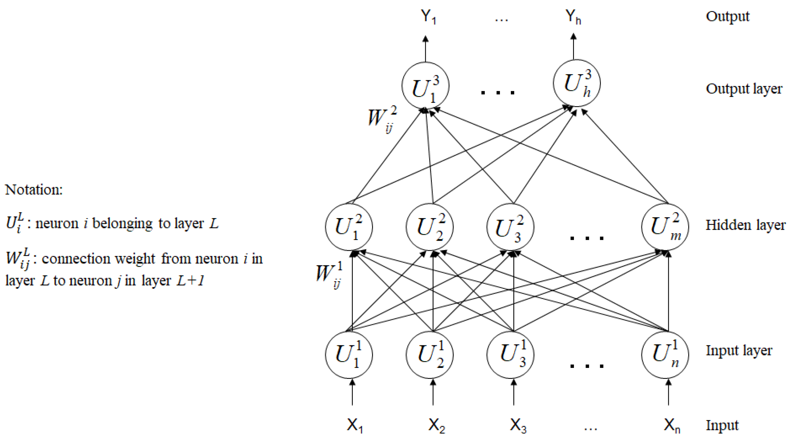
An MLP is a feed-forward neural network consisting of one input layer, at least one hidden layer, and one output layer. The input layer receives feature vectors (instances from the dataset) and passes them to the hidden layers without further computation. Hidden layers contain neurons that apply transformations to the inputs, with the number of neurons depending on the complexity of the task. The output layer generates the final predictions, consisting of one or more neurons depending on the classification problem (binary or multiclass).

Neurons in hidden and output layers operate on continuous-valued inputs and produce continuous outputs. Each neuron computes a weighted sum of its inputs, applies a nonlinear activation function, and transmits the result to the next layer.

Formally, the architecture of an MLP can be represented as a directed acyclic graph (DAG), where vertices correspond to neurons and edges correspond to weighted connections. Each layer forms an independent set of vertices, and edges exist only from one layer to the next, ensuring a layered and feed-forward structure. In an MLP, every vertex in layer $L_k$ has an outgoing edge to every vertex in layer $L_{k+1}$.

Weights on the edges are optimized using the backpropagation algorithm, which iteratively updates parameters to minimize the mean squared error (or another suitable loss function) between predicted and target outputs. The general architecture of the MLP is depicted in Figure 3.

This architecture was selected as a benchmark due to its flexibility, generalization ability, and interpretability in binary classification tasks. The MLP classifier was chosen because it provides a controlled, non-linear decision boundary capable of capturing complex interactions among features in the Pima dataset. Unlike logistic regression, which assumes linear separability, the MLP can model higher-order feature dependencies that are relevant for diabetes prediction (e.g., glucose–insulin interactions). Tree-based methods (e.g., Random Forest or XGBoost) were considered but were intentionally excluded to avoid confounding the evaluation of oversampling performance with model-specific ensembling or feature-splitting biases. Using a single classifier ensures that differences in performance can be attributed primarily to the data augmentation method rather than differences in model architecture. Moreover, MLPs are widely used as baseline neural models in studies evaluating GAN- or SMOTE-based augmentation, making results directly comparable to existing literature.

To ensure robust evaluation and mitigate overfitting, we employ 10-fold stratified cross-validation for all classification experiments. This approach partitions the dataset into 10 folds while preserving class distribution in each fold, ensuring that both majority and minority classes are represented proportionally across all folds. For each fold, the model is trained on 9 folds and evaluated on the remaining fold, and performance metrics (accuracy, precision, sensitivity, F1 Score) are averaged across all 10 folds with standard deviations reported. This stratified approach ensures that minority class instances are distributed across folds, preventing scenarios where some folds contain too few minority samples for meaningful evaluation.

To assess whether differences in performance metrics between augmentation methods are statistically significant, we employ two complementary statistical tests: the independent samples t-test and the Wilcoxon signed-rank test. The t-test evaluates whether the means of two independent samples are significantly different, assuming normality and equal variances, with the test statistic defined as

$$t={\displaystyle \frac{{\overline{X}}_1-{\overline{X}}_2}{s_p\sqrt{\frac{1}{n_1}+\frac{1}{n_2}}}},$$

where ${\overline{X}}_1$ and ${\overline{X}}_2$ are sample means, $s_p$ is the pooled standard deviation, and $n_1,n_2$ are sample sizes. In contrast, the Wilcoxon signed-rank test is a non-parametric alternative that does not assume normality and is therefore more robust to violations of distributional assumptions. This test ranks the absolute differences between paired observations and computes the test statistic as the sum of ranks for positive differences, making it particularly suitable for small samples or non-normally distributed data. Both tests are conducted at a significance level of $\alpha =0.05$, with rejection of the null hypothesis indicating a statistically meaningful difference between methods.

3. Results and Discussion

3.1. The Balanced Datasets from ctGAN and SMOTE Techniques

In supervised classification, maintaining class balance is critical to avoid model bias toward the majority class, reduce the risk of overfitting, and ensure fair evaluation across classes. Balanced datasets facilitate more reliable feature relevance analysis and improve the interpretability of classification outcomes.

As noted earlier, we employ the Pima Indians Diabetes dataset, a binary classification task for diagnosing diabetes mellitus in Indian women above 21 years of age. Table 2 shows the strong class imbalance: the majority class (class 0, negative cases) accounts for 65.10% of instances, while the minority class (class 1, positive cases) represents only 34.90%.

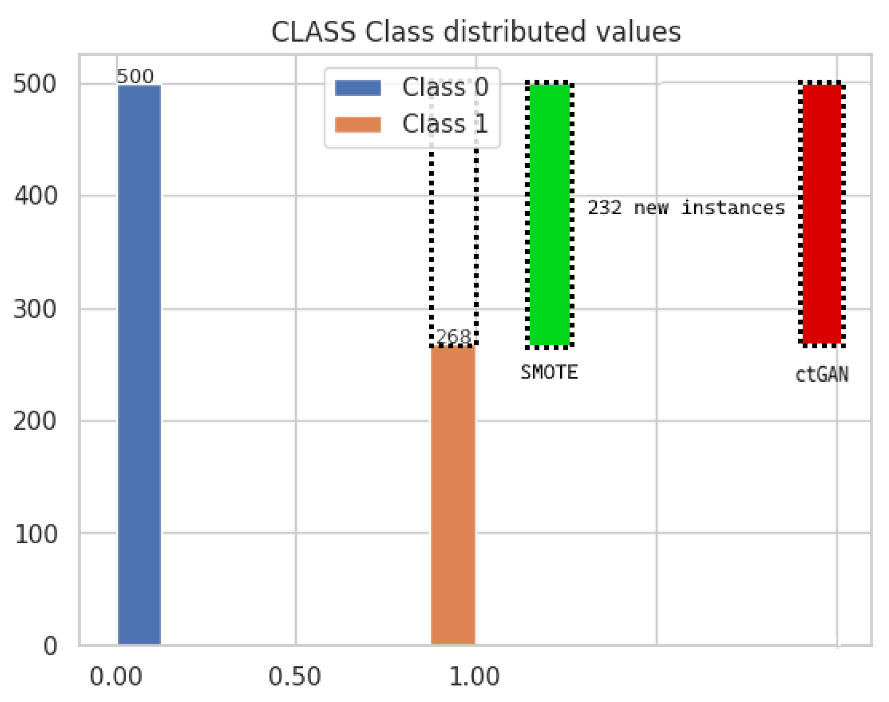
To address this imbalance, we independently applied the conditional tabular GAN (ctGAN) and the Synthetic Minority Oversampling Technique (SMOTE), generating two augmented datasets in which both classes contain 500 instances each (Figure 4). Both methods act as oversampling strategies, increasing the size of the minority class while preserving the majority class.

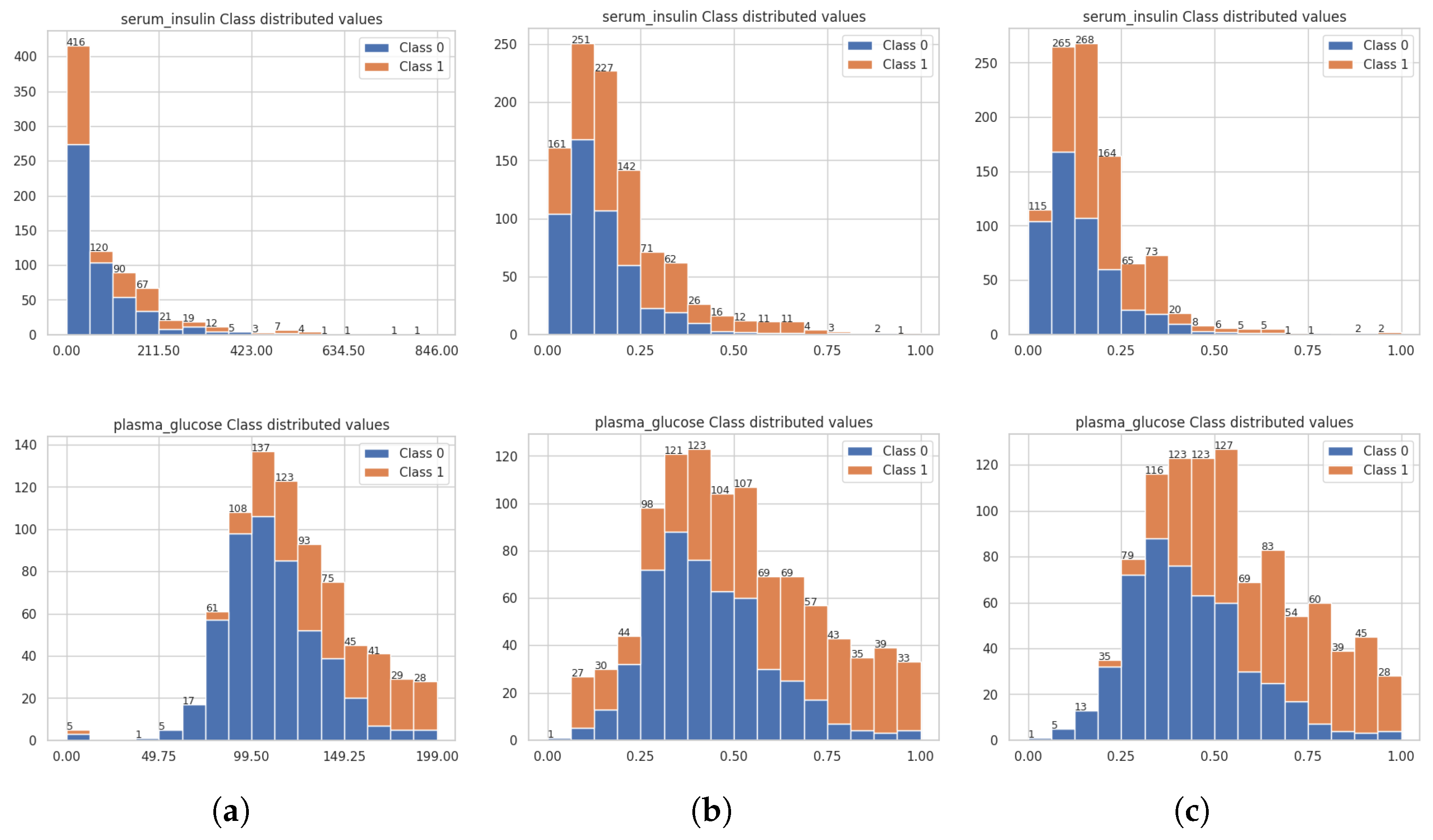
Figure 5 depicts the distributions of serum_insulin and plasma_glucose across the original dataset, the ctGAN-augmented dataset, and the SMOTE-augmented dataset, after imputation and scaling.

3.2. Assessing the Quality of the Balanced Datasets from ctGAN and SMOTE Techniques

The objective of this section is to evaluate how closely the datasets generated by ctGAN and SMOTE reproduce the statistical characteristics of the original Pima Indians Diabetes dataset. We assess similarity using visual inspection through Kernel Density Estimation (KDE) plots and quantitative distance-based metrics. This combined strategy allows us to examine both distributional shape and statistical fidelity. Throughout this section we focus on the eight features: age, body mass index (BMI), diabetes pedigree (DP), diastolic blood pressure (Diast), plasma glucose (PG), serum insulin (SI), skin thickness (ST), and times pregnant (TP).

Figure 6 presents the KDE curves for all eight features, comparing the original dataset with the ctGAN- and SMOTE-augmented versions under two preprocessing conditions (imputed only and imputed plus MinMax-normalized). Across most panels, both methods preserve the overall shape of the marginal distributions, with ctGAN displaying slightly broader tails for age and BMI (Figure 6a–d). Figure 5 complements this analysis by displaying class-wise distributions for two representative features, serum_insulin (SI) and plasma_glucose (PG), in the original, ctGAN-augmented, and SMOTE-augmented datasets. These plots confirm that both augmentation techniques maintain class-specific differences after balancing while modifying the minority-class support.

To quantify these observations,

Table 3. Statistical comparison of Pima Indians Diabetes dataset features across data augmentation methods. Both ctGAN and SMOTE effectively preserve the original feature support with minimal changes in central tendency and dispersion. In particular, ctGAN exhibits slightly higher variance in age (std: 13.342 vs. 11.753 in the original dataset) and comparable mean values for plasma_glucose (125.141 vs. 121.586 in the original dataset), while SMOTE remains closer to the original moments in most cases.

Feature	Dataset Type	Data Type	Mean	Std Dev	Min	Max
Age	Original	Imputed	33.241	11.753	21.000	81.000
	SMOTE	Imputed	33.982	11.308	21.000	81.000
	ctGAN	Imputed	35.487	13.342	21.000	81.000
	Original	Normalized	0.204	0.196	0.000	1.000
	SMOTE	Normalized	0.216	0.188	0.000	1.000
	ctGAN	Normalized	0.241	0.222	0.000	1.000
BMI	Original	Imputed	32.433	6.890	18.200	67.100
	SMOTE	Imputed	33.017	6.646	18.200	67.100
	ctGAN	Imputed	33.222	7.384	18.200	67.100
	Original	Normalized	0.291	0.141	0.000	1.000
	SMOTE	Normalized	0.304	0.138	0.000	1.000
	ctGAN	Normalized	0.307	0.151	0.000	1.000
Diabetes Pedigree	Original	Imputed	0.472	0.331	0.078	2.420
	SMOTE	Imputed	0.485	0.332	0.078	2.420
	ctGAN	Imputed	0.498	0.345	0.078	2.420
	Original	Normalized	0.195	0.137	0.000	1.000
	SMOTE	Normalized	0.201	0.137	0.000	1.000
	ctGAN	Normalized	0.206	0.143	0.000	1.000
Diastolic BP	Original	Imputed	69.105	19.356	24.000	122.000
	SMOTE	Imputed	70.234	18.987	24.000	122.000
	ctGAN	Imputed	71.156	19.543	24.000	122.000
	Original	Normalized	0.470	0.197	0.000	1.000
	SMOTE	Normalized	0.477	0.194	0.000	1.000
	ctGAN	Normalized	0.482	0.199	0.000	1.000
Plasma Glucose	Original	Imputed	121.586	30.542	44.000	199.000
	SMOTE	Imputed	126.071	31.211	44.000	199.000
	ctGAN	Imputed	125.141	32.203	44.000	199.000
	Original	Normalized	0.500	0.197	0.000	1.000
	SMOTE	Normalized	0.530	0.202	0.000	1.000
	ctGAN	Normalized	0.523	0.208	0.000	1.000
Serum Insulin	Original	Imputed	79.799	115.176	14.000	846.000
	SMOTE	Imputed	82.156	112.543	14.000	846.000
	ctGAN	Imputed	83.234	118.987	14.000	846.000
	Original	Normalized	0.078	0.138	0.000	1.000
	SMOTE	Normalized	0.081	0.135	0.000	1.000
	ctGAN	Normalized	0.082	0.143	0.000	1.000
Skin Thickness	Original	Imputed	20.536	15.952	7.000	99.000
	SMOTE	Imputed	21.234	16.123	7.000	99.000
	ctGAN	Imputed	21.987	16.543	7.000	99.000
	Original	Normalized	0.147	0.173	0.000	1.000
	SMOTE	Normalized	0.152	0.175	0.000	1.000
	ctGAN	Normalized	0.157	0.180	0.000	1.000
Times Pregnant	Original	Imputed	3.845	3.370	0.000	17.000
	SMOTE	Imputed	3.912	3.234	0.000	17.000
	ctGAN	Imputed	4.156	3.543	0.000	17.000
	Original	Normalized	0.226	0.198	0.000	1.000
	SMOTE	Normalized	0.230	0.190	0.000	1.000
	ctGAN	Normalized	0.245	0.208	0.000	1.000

reports summary statistics (mean, standard deviation, and support) for each feature under the three dataset types (original, SMOTE-augmented, and ctGAN-augmented) and the two preprocessing schemes (imputed and imputed plus MinMax-normalized). Both augmented datasets retain the original support, ensuring biological plausibility. SMOTE tends to reproduce means and variances more closely, whereas ctGAN introduces moderate additional variability in several features, most notably age and BMI, consistent with its generative nature and the broader tails observed in Figure 6.

A more detailed evaluation is provided in

Table 4. Comparison of distance metrics between original and augmented datasets across features. Abbreviations: EMD (Earth Mover’s Distance/Wasserstein), KS (Kolmogorov–Smirnov), JS (Jensen–Shannon), KL (Kullback–Leibler), AD (Anderson–Darling). Features: DP (Diabetes Pedigree), Diast (Diastolic BP), PG (Plasma Glucose), SI (Serum Insulin), ST (Skin Thickness), TP (Times Pregnant).

Metric	Comparison	Age	BMI	DP	Diast	PG	SI	ST	TP
EMD	ctGAN-Imp	2.249	0.797	0.036	1.773	3.560	21.124	0.690	0.349
	SMOTE-Imp	0.988	0.626	0.011	0.607	4.489	10.929	0.855	0.267
	ctGAN-Imp+Norm	0.037	0.016	0.015	0.018	0.023	0.027	0.007	0.021
	SMOTE-Imp+Norm	0.016	0.013	0.006	0.008	0.029	0.012	0.010	0.015
KS	ctGAN-Imp	0.062	0.042	0.038	0.066	0.051	0.083	0.053	0.047
	SMOTE-Imp	0.064	0.054	0.028	0.035	0.066	0.062	0.055	0.056
	ctGAN-Imp+Norm	0.062	0.042	0.038	0.068	0.052	0.085	0.044	0.047
	SMOTE-Imp+Norm	0.066	0.052	0.036	0.039	0.066	0.063	0.057	0.058
JS	ctGAN-Imp	0.095	0.077	0.080	0.062	0.066	0.099	0.069	0.054
	SMOTE-Imp	0.067	0.057	0.043	0.037	0.062	0.060	0.055	0.216
	ctGAN-Imp+Norm	0.095	0.077	0.080	0.066	0.067	0.101	0.039	0.054
	SMOTE-Imp+Norm	0.077	0.054	0.042	0.040	0.063	0.063	0.057	0.222
KL	ctGAN-Imp	0.031	0.019	0.020	0.015	0.016	0.035	0.037	0.012
	SMOTE-Imp	0.018	0.013	0.007	0.005	0.015	0.014	0.012	0.138
	ctGAN-Imp+Norm	0.031	0.019	0.020	0.016	0.017	0.035	0.006	0.012
	SMOTE-Imp+Norm	0.023	0.011	0.007	0.006	0.016	0.015	0.013	0.145
AD	ctGAN-Imp	6.503	1.710	0.547	4.842	2.308	8.081	0.588	1.594
	SMOTE-Imp	2.851	1.848	−0.659	−0.298	4.938	3.510	1.890	1.508
	ctGAN-Imp+Norm	6.503	1.774	0.547	4.988	2.346	8.238	0.264	1.594
	SMOTE-Imp+Norm	3.073	1.781	−0.214	0.280	4.910	3.573	2.045	1.496

, which summarizes four distance metrics between the original and augmented datasets: Kolmogorov–Smirnov (KS), Earth Mover’s Distance (EMD), Jensen–Shannon divergence (JS), and Kullback–Leibler divergence (KL), together with the Anderson–Darling (AD) statistic. These distances were computed under two conditions: (i) imputed data only and (ii) imputed plus MinMax-normalized data. Across most features, SMOTE yields smaller EMD and KL values than ctGAN, indicating closer distributional fidelity to the original dataset, particularly for BMI, diabetes_pedigree (DP), and skin_thickness (ST). In contrast, ctGAN exhibits larger divergences for long-tailed variables such as serum_insulin (SI), reflecting the broader variability already observed in Figure 6.

Normalization generally reduces the magnitude of the distance metrics for both augmentation methods, especially in terms of EMD and KL, confirming that part of the observed divergence is scale-dependent rather than structural. Nonetheless, residual differences persist for features with skewed or heavy-tailed distributions, as captured by the KS, JS, and AD statistics in Table 4. These discrepancies are expected when rebalancing datasets with heterogeneous minority-class structure and highlight that perfect alignment at the marginal level is neither guaranteed nor necessarily desirable in the presence of clinical variability.

Overall, the visual and quantitative evidence in Figure 5 and Figure 6 and Table 3 and Table 4 indicates that both ctGAN and SMOTE generate statistically coherent synthetic data. SMOTE more closely matches the marginal distributions of the original dataset for most features, whereas ctGAN introduces additional variability that may become useful in tasks requiring richer minority-class representation.

While the observed greater variability in ctGAN-generated samples (as reflected in larger standard deviations for features such as age and BMI) could indicate exploration of the latent space and potentially richer representation of minority cases, it is important to recognize that variability alone does not guarantee clinically valid diversity. Without additional validation, such variability may reflect training instabilities, mode collapse artifacts, or random noise rather than meaningful coverage of clinically relevant minority subpopulations. However, when the data are normalized beforehand, this effect is noticeably reduced. To strengthen the clinical relevance of ctGAN-generated samples, future work should incorporate phenotype clustering analysis or expert clinical annotation to verify whether observed variability corresponds to plausible minority subtypes (e.g., distinct diabetes phenotypes) or represents training artifacts. In this study, we acknowledge this limitation and focus on statistical validation through distributional comparisons and distance metrics, leaving comprehensive clinical validation for future research.

3.3. Analysis of the Accuracy of the Supervised Classification on the Original Dataset

Figure 7 displays the confusion matrices of the MLP classifier under three scenarios: (a) the original dataset, (b) the dataset with imputed values, and (c) the dataset with imputed and normalized values. The corresponding accuracies were 64.58%, 65.10%, and 73.96%, respectively.

The imbalance of the original dataset severely limited the model’s ability to detect positive cases (class 1). As shown in Figure 7a,b, the MLP correctly classified 98.69% and 100% of the negative cases (class 0) in the first two scenarios, while misclassifying the majority of positive cases. This behavior illustrates the classifier’s bias toward the majority class.

After imputation and normalization, a clear improvement was observed (Figure 7c), with the MLP showing a greater ability to separate classes 0 and 1. Nevertheless, 41.41% of positive cases continued to be incorrectly labeled as negative, highlighting the limitations of relying solely on preprocessing when the class distribution remains imbalanced. A more detailed evaluation of this setting, based on precision, sensitivity, and F1 Score, is provided in Section 3.6.

3.4. Analysis of the Accuracy of the Supervised Classification on the ctGAN-Augmented Dataset

Figure 8 presents the confusion matrices of the MLP classifier applied to (a) the ctGAN-augmented dataset, (b) the ctGAN-augmented dataset with imputed values, and (c) the ctGAN-augmented dataset with imputed and normalized values. The corresponding accuracies were 55.60%, 65.80%, and 72.00%, respectively.

At first glance, these values appear lower than those obtained on the original dataset (Figure 7), which could suggest a decline in performance. However, inspection of the diagonals in Figure 8 indicates that the MLP achieved a more balanced classification of classes 0 and 1 when trained on the ctGAN-augmented data. In particular, Figure 8a,b show that positive cases (class 1) were no longer entirely misclassified as negatives, a limitation observed in Figure 7a,b.

Moreover, the clearer definition of the diagonal in Figure 8c highlights that normalization combined with imputation improved the MLP’s discrimination ability. These results emphasize that accuracy alone is insufficient to assess performance, underscoring the need for complementary metrics such as precision, sensitivity, and F1 Score, which will be analyzed in Section 3.6.

Overall, a pattern similar to the original dataset was observed: the ctGAN-augmented dataset with imputed and normalized values yielded the best results among the three scenarios.

3.5. Analysis of the Accuracy of the Supervised Classification on the SMOTE-Augmented Dataset

Figure 9 presents the confusion matrices of the MLP classifier trained on (a) the SMOTE-augmented dataset, (b) the SMOTE-augmented dataset with imputed values, and (c) the SMOTE-augmented dataset with imputed and normalized values. The corresponding accuracies were 72.10%, 67.20%, and 78.00%, respectively.

Compared with the results on the ctGAN-augmented dataset (Figure 8), the SMOTE-augmented dataset consistently produced higher accuracy values. This indicates that the synthetic samples generated by SMOTE provided a closer approximation to the underlying data distribution, improving the model’s ability to classify both classes.

Among the three scenarios, the best performance was obtained with the imputed and normalized dataset (Figure 9c), a trend consistent with that observed for the original and ctGAN-augmented datasets.

3.6. Performance Assessment Metrics for MLP on Original, SMOTE-Augmented, and ctGAN-Augmented Datasets

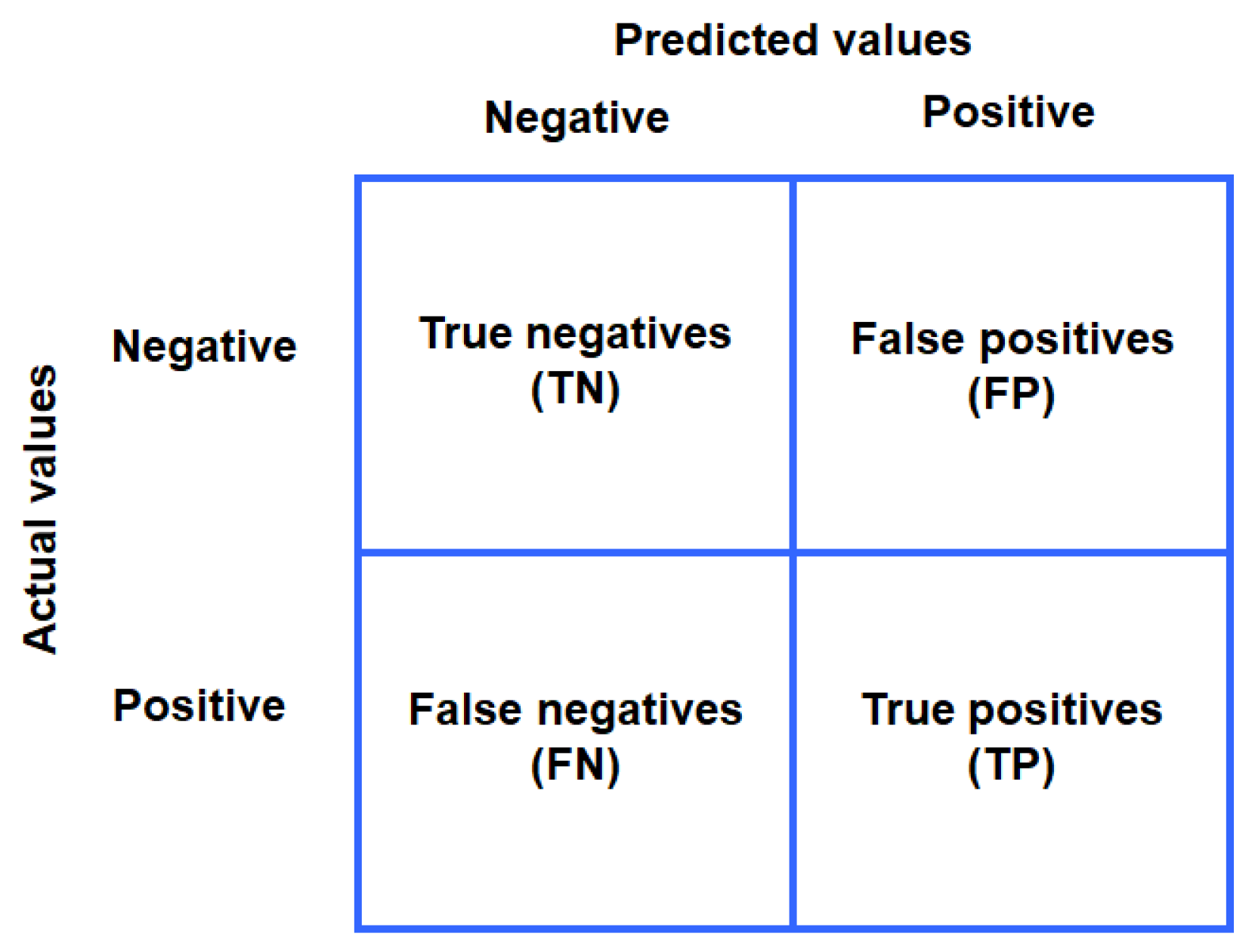
A confusion matrix provides a compact representation of the performance of a supervised classifier by reporting the number of correctly and incorrectly predicted instances across all classes (Figure 10). Rows correspond to the true classes and columns to the predicted classes.

From the entries of the confusion matrix, several evaluation metrics can be derived. The most commonly used are

• Accuracy: overall proportion of correct predictions

  $$Accuracy={\displaystyle \frac{TP+TN}{TP+TN+FP+FN}}.$$
• Precision: proportion of predicted positives that are correct

  $$Precision={\displaystyle \frac{TP}{TP+FP}}.$$
• Recall (Sensitivity): proportion of actual positives detected

  $$Recall={\displaystyle \frac{TP}{TP+FN}}.$$
• F1 Score: harmonic mean of precision and recall

  $$F1Score={\displaystyle \frac{2·Precision·Recall}{Precision+Recall}}.$$

We now focus on the MLP results obtained on the imputed and normalized versions of the original, ctGAN-augmented, and SMOTE-augmented datasets (Figure 7c–Figure 9c).

Table 5. Performance comparison across datasets using accuracy, F1-score, precision, and recall (mean ± standard deviation).

Dataset	Accuracy (%)	F1 (%)	Precision (%)	Recall (%)
PIMA imputed values	65.1059 ± 0.0068	51.3468 ± 0.0087	42.3890 ± 0.0089	65.1059 ± 0.0068
PIMA imputed GAN	63.8000 ± 0.1382	60.7102 ± 0.1765	69.7921 ± 0.1655	63.8000 ± 0.1382
PIMA imputed SMOTE	66.9000 ± 0.0896	65.2231 ± 0.1131	70.4216 ± 0.0808	66.9000 ± 0.0896
PIMA imputed GAN norm	70.5000 ± 0.1593	68.8825 ± 0.2008	74.0516 ± 0.1228	70.5000 ± 0.1593
PIMA imputed SMOTE norm	77.3000 ± 0.1203	77.1173 ± 0.1213	78.2555 ± 0.1280	77.3000 ± 0.1203

summarizes the corresponding performance metrics.

When comparing the three imputed datasets, clear differences emerge in classifier performance. The baseline imputed dataset shows the lowest performance across all metrics, with an accuracy of 65.10%, an F1 score of 51.35%, and a precision of 42.39%. Introducing ctGAN-based augmentation increases F1 to 60.71% and substantially improves precision to 69.79%, while maintaining similar accuracy and recall levels to the baseline. However, SMOTE augmentation produces the strongest overall performance. The SMOTE-augmented dataset achieves the highest accuracy (66.90%), highest F1 score (65.22%), and highest precision (70.42%) among the three approaches, indicating more balanced improvements across metrics. These results suggest that, while ctGAN introduces beneficial variability that enhances certain metrics, SMOTE more consistently improves classifier performance relative to both the original imputed dataset and the ctGAN-augmented version.

The comparison between the normalized ctGAN-augmented dataset and the normalized SMOTE-augmented dataset shows a clear advantage for SMOTE across all evaluation metrics, while ctGAN normalization improves performance relative to its non-normalized version, it still remains below SMOTE. The SMOTE-normalized dataset achieves the highest accuracy (77.30%), highest F1 score (77.12%), and highest precision (78.26%), with corresponding gains over ctGAN of approximately +6.8 percentage points in accuracy and +8.2 points in F1. Recall follows the same pattern, with SMOTE reaching 77.30% compared to 70.50% for ctGAN. These results indicate that, under normalization, SMOTE delivers more consistent and robust improvements in classifier performance, whereas ctGAN, although competitive, does not match the overall predictive strength obtained with SMOTE-based oversampling.

Statistical significance analysis was conducted using paired t-tests and Wilcoxon signed-rank tests across cross-validation folds to compare classifier performance under the two augmentation strategies. For both the imputed datasets (ctGAN vs. SMOTE) and the imputed-and-normalized datasets, no statistically significant differences were observed in accuracy, weighted F1, precision, or recall (all p-values > 0.065). These results indicate that both ctGAN- and SMOTE-based augmentation yield statistically equivalent classifier performance across evaluation metrics.

In summary, the comparative analysis highlights clear differences across the three datasets. The MLP trained on the original dataset suffered from limited sensitivity due to class imbalance, despite reporting moderate accuracy. The ctGAN-augmented dataset provided more balanced predictions, improving precision and recall, but still fell short of optimal performance. By contrast, the SMOTE-augmented dataset consistently achieved the best overall results across all evaluation metrics, confirming its effectiveness in producing synthetic data that preserves the statistical properties of the original distribution while enhancing classification performance.

3.7. Implications and Positioning Relative to Alternative Generative Approaches

The comparative results presented in this study provide clear evidence regarding the relative performance of SMOTE and ctGAN for medical data augmentation. However, the emerging landscape of generative methods invites discussion of their respective positions within a broader methodological context. As noted by Liu et al. [19], diffusion-based probabilistic models have demonstrated remarkable robustness in scenarios with limited training data, achieving consistent performance improvement even when traditional attention-based architectures deteriorate. This observation is particularly relevant for medical datasets, which often suffer from scarcity of high-quality labeled samples. The differences observed between SMOTE and ctGAN in our study can be understood through the lens of their underlying generative principles: SMOTE’s deterministic interpolation within the convex hull of existing minority instances ensures high fidelity to the empirical distribution, making it well-suited for datasets where minority patterns are relatively homogeneous and low-dimensional. In contrast, ctGAN’s adversarial training introduces greater variability, which may be advantageous when richer representation of minority subpopulations is required. However, this variability comes at a potential cost: as evidenced in Table 4, ctGAN exhibits larger distributional divergences (particularly in Wasserstein and Anderson–Darling metrics), suggesting that the synthetic samples, while diverse, may not maintain as tight a correspondence to the original data distribution. Looking forward, diffusion-based methods merit investigation in medical contexts where both stability and diversity are critical. Liu et al. have shown that diffusion models can achieve superior feature extractability in resource-constrained settings [19], a property that could prove invaluable in clinical applications where data scarcity is endemic. Nevertheless, the application of diffusion models to medical tabular data remains underexplored, and systematic comparative evaluation against established methods like SMOTE and ctGAN is warranted before widespread adoption in clinical practice.

4. Conclusions

This study aims to clarify how well–known techniques behave when evaluated under a standardized and statistically rigorous setting. By contrasting SMOTE and ctGAN across both distributional similarity and classifier performance, the results help contextualize prior reports in the literature and offer practical guidance for researchers working with limited or imbalanced medical datasets.

Among the two methods, SMOTE consistently outperformed ctGAN in terms of accuracy, sensitivity, and F1 Score, confirming its effectiveness in generating synthetic samples that closely approximate the minority class distribution. ctGAN, on the other hand, produced greater variability in the synthetic data, which may be advantageous in settings requiring richer representation of minority cases. From a mathematical standpoint, this comparison can be interpreted as evaluating how closely the synthetic distributions $Q_X$ generated by each method approximate the original distribution $P_X$ under suitable distance measures (e.g., Kolmogorov–Smirnov, Integrated Squared Error, or information-theoretic divergences) or descriptive statistical measures. This perspective emphasizes that oversampling is not merely a data manipulation procedure, but rather an attempt to approximate probability distributions governing the real data.

The observed differences between SMOTE and ctGAN reflect the distinct strengths of each approach rather than a strict performance hierarchy. SMOTE’s deterministic interpolation produces highly stable synthetic samples that closely follow the local structure of the minority class, which explains its strong performance on a dataset like PIMA, where minority patterns are relatively simple and well captured by k-nearest neighbors. ctGAN, in contrast, introduces greater variability due to adversarial training, which can slightly increase divergence metrics but also enables the modeling of more complex or nonlinear patterns that SMOTE cannot represent. In this sense, both methods remain valuable: SMOTE offers stability and strong local fidelity, while ctGAN provides generative flexibility that becomes advantageous when richer variability or more complex class structure is present.

The quantitative evaluation using various distance metrics (Kolmogorov–Smirnov, Wasserstein, Anderson–Darling, Jensen–Shannon, among others) confirms that both SMOTE and ctGAN effectively produced high-quality synthetic data. Both approaches effectively conserved the marginal distributions of features with commendable integrity, sustained feature support within observed biological ranges, and consistently recreated the statistical properties of the original dataset. SMOTE demonstrated a marginally more robust valid alternative that enhances minority class representation. These findings validate that both augmentation techniques are feasible and efficacious for mitigating class imbalance in medical datasets.

The study is not without limitations. First, the analysis was conducted on a single dataset with specific demographic characteristics (Indian women aged 21 and older), which limits the generalizability of our findings. An important limitation is that we do not address whether synthetic augmentation maintains robustness when applied to external cohorts with different demographic profiles, comorbidities, or clinical settings. Second, while our evaluation framework includes multiple statistical distances and classification metrics, it remains limited to static measures that do not assess model calibration or inter-cohort generalizability. Future work should include the external validation on independent datasets with varying demographic compositions and clinical contexts, the assessment of model calibration to ensure predicted probabilities are well-calibrated and clinically interpretable, and an evaluation of inter-cohort generalizability to verify that improvements in sensitivity and F1 score extend beyond the specific dataset used in this study. Additionally, broader validation on diverse medical datasets and exploration of additional methods, including hybrid approaches that combine interpolation and generative modeling, constitute promising avenues for future research. Recent comprehensive reviews have highlighted the persistent challenges in handling imbalanced medical datasets [24], emphasizing the need for continued methodological comparatives. Without such comprehensive validation, conclusions may remain dataset-specific and may not be directly applicable to broader clinical practice but the methodology described in this work still provides a robust and transferable framework for generating and evaluating synthetic clinical data.

Future work should validate our findings across multiple medical datasets with varying class imbalance ratios and demographic characteristics to establish generalizability. External validation on independent cohorts would clarify whether the observed advantages of SMOTE extend beyond the Pima dataset. Additionally, systematic comparison with emerging diffusion-based methods and other generative approaches would enrich the landscape of medical data augmentation techniques. Finally, investigation of hybrid approaches combining interpolation and generative modeling, along with incorporation of domain expertise for clinical validation, would strengthen confidence in synthetic data quality and ensure that improvements translate to clinically meaningful gains in real-world deployment.

Furthermore, our study focuses on two representative oversampling strategies (SMOTE and ctGAN) as a way to contrast a deterministic, interpolation-based method with a modern generative approach tailored to tabular data. Although other families of models like diffusion-based generators, variational autoencoders, or flow-based architectures. These alternatives may provide complementary benefits in terms of stability, diversity, or scalability, and a broader benchmarking effort would undoubtedly enrich the landscape of medical data augmentation. We suggest this as a natural direction for future research.

This study demonstrates that both SMOTE and ctGAN are effective techniques for mitigating class imbalance in medical diagnostic datasets. The thorough distributional analysis verifies that both methods provide synthetic data of superior statistical quality, effectively maintaining the attributes of the original data while improving minority class representation. Both techniques attain adequate authenticity, as confirmed by visual (KDE) and quantitative (distance-based) measures. This systematic comparison demonstrates that practitioners can reliably utilize either technique, choosing according to their particular needs for distributional accuracy or feature space variety. These findings highlight the need of stringent metric-based validation in augmentation studies and endorse the wider use of these methodologies in medical machine learning.

References

1. He, H.; Garcia, E. Learning from Imbalanced Data. IEEE Trans. Knowl. Data Eng. 2009, 21, 1263–1284. [Google Scholar] [CrossRef]
2. Thabtah, F.; Hammoud, S.; Kamalov, F.; Gonsalves, A. Data imbalance in classification: Experimental evaluation. Inf. Sci. 2020, 513, 429–441. [Google Scholar] [CrossRef]
3. Yang, Y.; Hsee, C.K.; Li, X. Prediction Biases: An Integrative Review. Curr. Dir. Psychol. Sci. 2021, 30, 195–201. [Google Scholar] [CrossRef]
4. Mohammed, R.; Rawashdeh, J.; Abdullah, M. Machine Learning with Oversampling and Undersampling Techniques: Overview Study and Experimental Results. In Proceedings of the 2020 11th International Conference on Information and Communication Systems (ICICS), Irbid, Jordan, 7–9 April 2020; IEEE: Piscataway, NJ, USA, 2020; pp. 243–248. [Google Scholar] [CrossRef]
5. Thai-Nghe, N.; Gantner, Z.; Schmidt-Thieme, L. Cost-sensitive learning methods for imbalanced data. In Proceedings of the 2010 International Joint Conference on Neural Networks (IJCNN), Barcelona, Spain, 18–23 July 2010; IEEE: Piscataway, NJ, USA, 2010; pp. 1–8. [Google Scholar] [CrossRef]
6. Qian, Y.; Liang, Y.; Li, M.; Feng, G.; Shi, X. A resampling ensemble algorithm for classification of imbalance problems. Neurocomputing 2014, 143, 57–67. [Google Scholar] [CrossRef]
7. Wong, S.C.; Gatt, A.; Stamatescu, V.; McDonnell, M.D. Understanding Data Augmentation for Classification: When to Warp? In Proceedings of the 2016 International Conference on Digital Image Computing: Techniques and Applications (DICTA), Gold Coast, Australia, 30 November–2 December 2016; IEEE: Piscataway, NJ, USA, 2016; pp. 1–6. [Google Scholar] [CrossRef]
8. Afzal, S.; Maqsood, M.; Nazir, F.; Khan, U.; Aadil, F.; Awan, K.M.; Mehmood, I.; Song, O.Y. A Data Augmentation-Based Framework to Handle Class Imbalance Problem for Alzheimer’s Stage Detection. IEEE Access 2019, 7, 115528–115539. [Google Scholar] [CrossRef]
9. Jiang, X.; Ge, Z. Data Augmentation Classifier for Imbalanced Fault Classification. IEEE Trans. Autom. Sci. Eng. 2021, 18, 1206–1217. [Google Scholar] [CrossRef]
10. Chawla, N.V.; Bowyer, K.W.; Hall, L.O.; Kegelmeyer, W.P. SMOTE: Synthetic Minority Over-sampling Technique. J. Artif. Intell. Res. 2002, 16, 321–357. [Google Scholar] [CrossRef]
11. Elreedy, D.; Atiya, A.F. A Comprehensive Analysis of Synthetic Minority Oversampling Technique (SMOTE) for handling class imbalance. Inf. Sci. 2019, 505, 32–64. [Google Scholar] [CrossRef]
12. Wongvorachan, T.; He, S.; Bulut, O. A Comparison of Undersampling, Oversampling, and SMOTE Methods for Dealing with Imbalanced Classification in Educational Data Mining. Information 2023, 14, 54. [Google Scholar] [CrossRef]
13. Dablain, D.; Krawczyk, B. DeepSMOTE: Fusing Deep Learning and SMOTE for Imbalanced Data. IEEE Trans. Neural Netw. Learn. Syst. 2022, 34, 6390–6404. [Google Scholar] [CrossRef]
14. Wang, K.; Gou, C.; Duan, Y.; Lin, Y.; Zheng, X.; Wang, F.Y. Generative adversarial networks: Introduction and outlook. IEEE/CAA J. Autom. Sin. 2017, 4, 588–598. [Google Scholar] [CrossRef]
15. Creswell, A.; White, T.; Dumoulin, V.; Arulkumaran, K.; Sengupta, B.; Bharath, A.A. Generative Adversarial Networks: An Overview. IEEE Signal Process. Mag. 2018, 35, 53–65. [Google Scholar] [CrossRef]
16. Goodfellow, I.; Pouget-Abadie, J.; Mirza, M.; Xu, B.; Warde-Farley, D.; Ozair, S.; Courville, A.; Bengio, Y. Generative adversarial networks. Commun. ACM 2020, 63, 139–144. [Google Scholar] [CrossRef]
17. Xu, L.; Skoularidou, M.; Cuesta-Infante, A.; Veeramachaneni, K. Modeling Tabular data using Conditional GAN. In Proceedings of the Advances in Neural Information Processing Systems, Vancouver, BC, Canada, 8–14 December 2019; Volume 32, pp. 27517–27529. [Google Scholar] [CrossRef]
18. Casanova, M.; Careil, M.; Verbeek, J.; Drozdzal, M.; Soriano, A.R. Instance-Conditioned GAN. In Proceedings of the Advances in Neural Information Processing Systems, Virtual, 6–14 December 2021; Volume 34, pp. 27517–27529. [Google Scholar] [CrossRef]
19. Liu, Y.; Liu, A.; Gao, S. A flame image soft sensor for oxygen content prediction based on denoising diffusion probabilistic model. Chemom. Intell. Lab. Syst. 2024, 255, 105269. [Google Scholar] [CrossRef]
20. Kingma, D.P.; Welling, M. Auto-encoding variational Bayes. arXiv 2022, arXiv:1312.6114. [Google Scholar]
21. Ahsan, M.M.; Luna, S.A.; Siddique, Z. Machine-Learning-Based Disease Diagnosis: A Comprehensive Review. Healthcare 2022, 10, 541. [Google Scholar] [CrossRef]
22. An, Q.; Rahman, S.; Zhou, J.; Kang, J.J. A Comprehensive Review on Machine Learning in Healthcare Industry: Classification, Restrictions, Opportunities and Challenges. Sensors 2023, 23, 4178. [Google Scholar] [CrossRef]
23. Uddin, S.; Khan, A.; Hossain, M.E.; Moni, M.A. Comparing different supervised machine learning algorithms for disease prediction. BMC Med. Inform. Decis. Mak. 2019, 19, 281. [Google Scholar] [CrossRef]
24. Salmi, M.; Atif, D.; Oliva, D.; Abraham, A.; Ventura, S. Handling imbalanced medical datasets: Review of a decade of research. Artif. Intell. Rev. 2024, 57, 163. [Google Scholar] [CrossRef]
25. Fujiwara, K.; Huang, Y.; Hori, K.; Nishioji, K.; Kobayashi, M.; Kamaguchi, M.; Kano, M. Over- and Under-sampling Approach for Extremely Imbalanced and Small Minority Data Problem in Health Record Analysis. Front. Public Health 2020, 8, 178. [Google Scholar] [CrossRef]
26. Rahman, M.M.; Davis, D.N. Addressing the Class Imbalance Problem in Medical Datasets. Int. J. Mach. Learn. Comput. 2013, 3, 224–228. [Google Scholar] [CrossRef]
27. Wang, Y.C.; Cheng, C.H. A multiple combined method for rebalancing medical data with class imbalances. Comput. Biol. Med. 2021, 134, 104527. [Google Scholar] [CrossRef] [PubMed]
28. Yang, W.; Pan, C.; Zhang, Y. An oversampling method for imbalanced data based on spatial distribution of minority samples SD-KMSMOTE. Sci. Rep. 2022, 12, 16820. [Google Scholar] [CrossRef] [PubMed]
29. Eom, G.; Byeon, H. Searching for Optimal Oversampling to Process Imbalanced Data: Generative Adversarial Networks and Synthetic Minority Over-Sampling Technique. Mathematics 2023, 11, 3605. [Google Scholar] [CrossRef]
30. Suresh, T.; Brijet, Z.; Subha, T.D. Imbalanced medical disease dataset classification using enhanced generative adversarial network. Comput. Methods Biomech. Biomed. Eng. 2023, 26, 1702–1718. [Google Scholar] [CrossRef]
31. Zhang, Y.; Wang, Z.; Zhang, Z.; Liu, J.; Feng, Y.; Wee, L.; Dekker, A.; Chen, Q.; Traverso, A. GAN-based one dimensional medical data augmentation. Soft Comput. 2023, 27, 10481–10491. [Google Scholar] [CrossRef]
32. Chang, V.; Bailey, J.; Xu, Q.A.; Sun, Z. Pima Indians diabetes mellitus classification based on machine learning (ML) algorithms. Neural Comput. Appl. 2023, 35, 16157–16173. [Google Scholar] [CrossRef]
33. Sankar Ganesh, P.V.; Sripriya, P. A Comparative Review of Prediction Methods for Pima Indians Diabetes Dataset. In Computational Vision and Bio-Inspired Computing; Smys, S., Tavares, J.M.R.S., Balas, V.E., Iliyasu, A.M., Eds.; Springer: Cham, Switzerland, 2020; pp. 735–750. [Google Scholar] [CrossRef]
34. Patra, R.; Khuntia, B. Analysis and Prediction Of Pima Indian Diabetes Dataset Using SDKNN Classifier Technique. IOP Conf. Ser. Mater. Sci. Eng. 2021, 1070, 012059. [Google Scholar] [CrossRef]
35. Xu, Z.; Shen, D.; Nie, T.; Kou, Y.; Yin, N.; Han, X. A cluster-based oversampling algorithm combining SMOTE and k-means for imbalanced medical data. Inf. Sci. 2021, 572, 574–589. [Google Scholar] [CrossRef]
36. Kishor, A.; Chakraborty, C. Early and accurate prediction of diabetics based on FCBF feature selection and SMOTE. Int. J. Syst. Assur. Eng. Manag. 2021, 15, 4649–4657. [Google Scholar] [CrossRef]
37. Blagus, R.; Lusa, L. SMOTE for high-dimensional class-imbalanced data. BMC Bioinform. 2013, 14, 106. [Google Scholar] [CrossRef]
38. Fernandez, A.; Garcia, S.; Herrera, F.; Chawla, N.V. SMOTE for Learning from Imbalanced Data: Progress and Challenges, Marking the 15-year Anniversary. J. Artif. Intell. Res. 2018, 61, 1–54. [Google Scholar] [CrossRef]
39. Gholampour, S. Impact of Nature of Medical Data on Machine and Deep Learning for Imbalanced Datasets: Clinical Validity of SMOTE Is Questionable. Mach. Learn. Knowl. Extr. 2024, 6, 827. [Google Scholar] [CrossRef]
40. Gardner, M.; Dorling, S. Artificial neural networks (the multilayer perceptron)—A review of applications in the atmospheric sciences. Atmos. Environ. 1998, 32, 2627–2636. [Google Scholar] [CrossRef]
41. Ramchoun, H.; Amine, M.; Idrissi, J.; Ghanou, Y.; Ettaouil, M. Multilayer Perceptron: Architecture Optimization and Training. Int. J. Interact. Multimed. Artif. Intell. 2016, 4, 26–30. [Google Scholar] [CrossRef]
Figure 1. Graphical representation of the SMOTE algorithm. The figure illustrates the interpolation process where synthetic samples (red points) are generated along line segments connecting a minority class instance (green points) to its k = 3 nearest neighbors (orange points) in the feature space. This deterministic interpolation ensures all synthetic samples lie within the convex hull of existing minority cases.
Mathematics 13 04032 g001
Figure 2. Structure of a Generative Adversarial Network, comprising a generator and a discriminator trained in opposition. The generator (left) maps noise z and conditioning c to synthetic samples x g e n , while the discriminator (right) distinguishes real ( x , c ) from generated ( x g e n , c ) samples. Training follows an adversarial minimax game over 1000 epochs with learning rates of 2 × 10 4 for both networks.
Mathematics 13 04032 g002
Figure 3. General structure of a multilayer perceptron network used for classification. The architecture consists of an input layer (8 neurons for 8 features), a hidden layer with 5 neurons (calculated as ( n f e a t u r e s + n c l a s s e s ) / 2 ), and an output layer (2 neurons for binary classification). Training uses the L-BFGS solver with tanh activation, adaptive learning rate (initial: 0.03), early stopping, and 10-fold stratified cross-validation.
Mathematics 13 04032 g003
Figure 4. Balanced datasets produced by the use of the ctGAN and SMOTE techniques, where the number of instances in both classes is the same. Starting from the original imbalanced dataset (268 minority, 500 majority), both methods generate 232 synthetic minority samples to achieve perfect class balance (500 instances per class). SMOTE uses k = 3 nearest neighbors for interpolation, while ctGAN employs conditional generation with constraints to maintain biological plausibility.
Mathematics 13 04032 g004
Figure 5. Class-wise distributions of serum_insulin (top row) and plasma_glucose (bottom row) in (a) the original dataset, (b) the ctGAN-augmented dataset, and (c) the SMOTE-augmented dataset. All datasets shown here have been preprocessed with KNN imputation (k = 3) and MinMax normalization. Class 0 (negative cases) is shown in blue, Class 1 (positive cases) in red. The distributions demonstrate how both augmentation methods preserve the class-specific feature characteristics while balancing class representation.
Mathematics 13 04032 g005
Figure 6. Kernel density plots for the eight attributes: age, BMI, diabetes_pedigree (DP), diastolic blood pressure (Diast), plasma_glucose (PG), serum_insulin (SI), skin_thickness (ST), times_pregnant (TP). Column (a) shows distributions after KNN imputation ( k = 3 ), while column (b) shows distributions after both imputation and MinMax normalization. In each subplot, the blue curve represents the original dataset, red represents SMOTE-augmented data (generated with k = 3 neighbors), and green represents ctGAN-augmented data (trained for 1000 epochs with architecture ( 5 , 5 ) ). The horizontal axis corresponds to the feature value and the vertical axis to the estimated density for that feature. The plots illustrate the distributional alignment of the synthetic samples with respect to the original data.
Mathematics 13 04032 g006
Figure 7. Confusion matrices for the original dataset evaluated using 10-fold stratified cross-validation: (a) MLP on the raw original dataset (no preprocessing), (b) MLP on the original dataset with KNN imputation (k = 3), and (c) MLP on the original dataset with both imputation and MinMax normalization. MLP configuration: hidden layer size = 5, activation = tanh, solver = L-BFGS, learning rate = adaptive (initial = 0.03), early stopping enabled. True negatives (TN) and true positives (TP) are shown on the diagonal.
Mathematics 13 04032 g007
Figure 8. Confusion matrices for the ctGAN-augmented dataset evaluated using 10-fold stratified cross-validation: (a) MLP on the raw augmented dataset (no preprocessing), (b) MLP on the augmented dataset with KNN imputation (k = 3), and (c) MLP on the augmented dataset with both imputation and MinMax normalization. The ctGAN was trained for 1000 epochs with generator/discriminator architecture ( 5 , 5 ) , learning rate 2 × 10 4 , batch size 100, and generated 232 synthetic minority samples. MLP configuration as in Figure 7.
Mathematics 13 04032 g008
Figure 9. Confusion matrices for the SMOTE-augmented dataset evaluated using 10-fold stratified cross-validation: (a) MLP on the raw augmented dataset (no preprocessing), (b) MLP on the augmented dataset with KNN imputation (k = 3), and (c) MLP on the augmented dataset with both imputation and MinMax normalization. SMOTE was applied with k = 3 nearest neighbors, generating 232 synthetic minority samples through linear interpolation. MLP configuration as in Figure 7.
Mathematics 13 04032 g009
Figure 10. Confusion matrix for binary classification showing the standard layout: True Negatives (TN) in the top-left, False Positives (FP) in the top-right, False Negatives (FN) in the bottom-left, and True Positives (TP) in the bottom-right. This matrix structure is used throughout the paper to evaluate MLP performance under different preprocessing and augmentation conditions.
Mathematics 13 04032 g010