Article

KAN-Former: 4D Trajectory Prediction for UAVs Based on Cross-Dimensional Attention and KAN Decomposition

College of Artificial Intelligence and Automation, Hohai University, Changzhou 213200, China
*
Author to whom correspondence should be addressed.
Mathematics 2025, 13(23), 3877; https://doi.org/10.3390/math13233877
Submission received: 17 October 2025 / Revised: 13 November 2025 / Accepted: 2 December 2025 / Published: 3 December 2025

Abstract

To address the core challenges of multivariate nonlinear coupling and long-term temporal dependency in 4D UAV trajectory prediction, this study proposes an innovative model named KAN-Former. On a 21-dimensional multimodal UAV dataset, KAN-Former achieves statistically significant improvements over all baseline models, reducing the mean squared error (MSE) by 8.96% compared to the standard Transformer and by 2.66% compared to the strongest physics-informed baseline (PITA), while decreasing the mean absolute error (MAE) by 7.43% relative to TimeMixer/PatchTST. The model adopts a collaborative architecture with two key components: first, a “vertical–horizontal” cross-dimensional attention mechanism—where the vertical branch models physical correlations among multivariate variables using hierarchical clustering priors, and the horizontal branch employs a blockwise dimensionality reduction strategy to efficiently capture long-term temporal dynamics; second, it represents the first application of Kolmogorov–Arnold decomposition in trajectory prediction, replacing traditional feedforward networks with learnable combinations of B-spline basis functions to approximate high-dimensional nonlinear mappings. Ablation studies verify the effectiveness of each module, with the KAN module alone reducing MSE by 6.59%. Moreover, the model’s feature clustering results align closely with UAV physical characteristics, significantly improving interpretability. The demonstrated improvements in accuracy, interpretability, and computational efficiency make KAN-Former highly suitable for real-world applications such as real-time flight control and air traffic management, providing reliable trajectory forecasts for decision-making systems. This work offers a new paradigm for trajectory prediction in complex dynamic systems, successfully integrating theoretical innovation with practical value.

1. Introduction

The rapid advancement of UAV (Unmanned Aerial Vehicle) technology has led to its extensive application in various fields, including logistics delivery, disaster relief, and precision agriculture. However, as mission scenarios become more complex, UAV trajectory prediction encounters two main challenges. (1) Strong Nonlinear Dynamic Coupling: During UAV flight, multiple variables such as position, attitude, and wind speed exhibit complex nonlinear interactions [1]. For instance, under the influence of wind field disturbances, the estimation error of propeller angular velocity can reach 0.15 rad/s, making it challenging for traditional linear models to achieve more accurate predictions. (2) Difficulty in Modeling Long-Term Temporal Dependencies: Existing methods often struggle to effectively capture dynamic patterns over extended periods, resulting in accumulated prediction errors [2]. Experimental results show that during 30 min flights, traditional methods can produce trajectory errors of up to 5 m and velocity errors of 0.1 m/s.
Current UAV trajectory prediction methods mainly fall into three categories: (1) State estimation-based methods, including Hidden Markov Models (HMM) [3], Particle Filters (PF) [4], and Kalman Filters (KF) [5], which recursively estimate states through kinematic equations. While computationally efficient, they rely on linear assumptions and are prone to significant error accumulation [6]. (2) Dynamics model-based approaches such as Model Predictive Control (MPC) [7] and Udwadia-Kalaba (U-K) equations [8], which model based on Newton–Euler equations with clear physical interpretability, but show poor adaptability to complex environmental disturbances (e.g., unsteady aerodynamic effects) [9,10]. (3) Deep learning-based methods. RNN/LSTM [11,12,13,14,15,16] models temporal dependencies through recursive structures but face gradient vanishing problems and struggle with long sequences (>500 steps). Transformer [17,18,19,20] utilizes self-attention mechanisms to capture global dependencies, but it has three key limitations: traditional attention mechanisms fail to model physical correlations among multivariate variables explicitly; single-dimensional attention has difficulty coordinating spatiotemporal features; and standard Feedforward Networks (FFN) possess limited expressive capability for high-dimensional nonlinear coupling.
To address these issues, this paper proposes KAN-Former for long-term UAV trajectory prediction with the following main innovations:
(1)
Methodological innovation: A cross-dimensional attention mechanism is proposed. Vertical attention explicitly models physical correlations among multivariate variables (e.g., attitude–wind speed coupling) based on hierarchical clustering priors. Horizontal attention, on the other hand, employs a blockwise dimensionality reduction strategy to capture long-term temporal dependencies efficiently.
(2)
Theoretical innovation: The Kolmogorov–Arnold decomposition theorem is introduced in trajectory prediction, replacing FFN with learnable B-spline basis function combinations to approximate high-dimensional nonlinear mappings through low-dimensional functions, avoiding the curse of dimensionality.
(3)
Performance improvement on 21-dimensional multimodal data. MSE is reduced by 8.96% compared to Transformer and MAE is reduced by 7.43% compared to TimeMixer. Feature clustering results enhance model interpretability, providing a physical basis for engineering deployment and informed decision-making.
The structure of the paper is as follows: Section 2 reviews related work and details the KAN-Former architecture. Section 3 validates its effectiveness through experiments. Section 4 concludes with a discussion of future directions.

2. Materials and Methods

2.1. Related Work

2.1.1. State Estimation-Based Methods

State estimation-based trajectory prediction models typically estimate target motion states by constructing kinematic equations that relate state variables, such as position, velocity, and acceleration. These methods establish state transition relationships using historical trajectory data, featuring simple model structures and high computational efficiency, without involving dynamic parameters such as aircraft mass or aerodynamic forces. Qiao et al. [3] employed the Hidden Markov Model (HMM) from statistics for predicting fighter aircraft trajectories, which can adaptively select appropriate parameters under different environmental conditions and effectively handle uncertainties and complexities in aircraft motion. Additionally, probabilistic estimation methods such as Particle Filters (PF) [4] and Kalman Filters (KF) [5], along with the Interactive Multiple Model (IMM) algorithm [21] for multiple motion patterns, form the primary technical framework for traditional trajectory prediction.
However, for highly maneuverable small UAVs, state estimation models struggle to ensure prediction accuracy, leading to error accumulation. Furthermore, high computational complexity makes it challenging to balance prediction time and accuracy. These methods are typically only suitable for short-term prediction [6].

2.1.2. Dynamics Model-Based Methods

Dynamics model-based trajectory prediction models establish kinematic equations incorporating real-time flight states, meteorological parameters, and flight intentions to predict trajectories. K et al. [7] proposed a dual Model Predictive Control (MPC) strategy for trajectory tracking of autonomous quadrotors, combining translational and attitude control and modeling via Piecewise Affine (PWA) systems to enhance robustness against atmospheric disturbances and physical constraints. K et al. [8] introduced a novel Udwadia-Kalaba (U-K) method for quadrotor trajectory tracking control, providing closed-form nonlinear control by solving U-K equations to achieve precise tracking of designed trajectories without imposing prior structural constraints. Baklacioglu’s team [9] employed a genetic algorithm optimization framework to achieve adaptive parameter matching for trajectory prediction during the transport aircraft’s climb and descent phases. Chao et al. [10] proposed a 4D trajectory prediction method based on fundamental flight models, constructing horizontal, vertical, and speed profiles of aircraft according to the characteristics of each flight phase.
While these methods have rigorous physical foundations in theory, they still face limitations: (1) For special platforms like rotorcraft UAVs, they fail to account for strong nonlinear dynamic coupling caused by unsteady aerodynamic effects, leading to fundamental deviations between models and actual motion characteristics; (2) Predefined settings obtained from existing databases or estimates are often insufficiently accurate. When data resources are limited or inadequate, prediction accuracy degrades significantly, rendering the models inapplicable.

2.1.3. Neural Network-Based Methods

Advancements in neural network technology have led to the widespread adoption of neural network-based methods for trajectory prediction. Recurrent Neural Networks (RNNs) are commonly used for predicting UAV trajectories due to their ability to capture temporal dependencies within the trajectory data [11,12,13]. However, RNNs can struggle to model long-term dependencies, particularly in complex flight environments. To overcome this limitation, Shi et al. [14] developed a 4D trajectory prediction model using Long Short-Term Memory (LSTM) networks, which enhanced the model’s ability to store and utilize long-term information effectively. Additionally, Han et al. [15] proposed a short-term 4D trajectory prediction model based on LSTM, which demonstrated improved performance for short-term predictions. Furthermore, Shi et al. [16] combined LSTM with differential autoregressive moving average (ARIMA) models to create a hybrid model. In this approach, LSTM serves as the primary predictive model, while ARIMA acts as an auxiliary model, partially addressing issues related to prediction accuracy and stability.
A limitation of LSTMs is their step-by-step computation, which consumes significant memory and computational resources for long sequences. In contrast, Transformers [17] can more efficiently capture global dependencies and enable parallel processing through self-attention mechanisms. Dong et al. [18] applied Transformer models to UAV trajectory optimization, proposing an Attention-based UAV Trajectory Optimization (AUTO) framework using graph Transformers. Li et al. [19] introduced a Transformer-Encoder-LSTM model, which leverages Transformers to capture long-range dependencies while utilizing LSTMs to handle missing trajectory data. Luo et al. [20] incorporated a trajectory stabilization module into Transformer models to ensure time-series stability, thereby improving predictability.
However, existing Transformer-based prediction methods still encounter two key challenges when addressing the complex and variable flight patterns of UAVs: (1) Traditional self-attention mechanisms often do not fully exploit the physical correlations between features, leading to inadequate local dynamic modeling; (2) Standard Feedforward Networks (FFN) find it challenging to approximate complex relationships in high-dimensional sensor data accurately.
To systematically analyze the characteristics and limitations of existing methods, Table 1 compares representative models across various dimensions, including multivariate modeling and long-term sequence processing.
As shown in Table 1, early RNN/LSTM models temporal dependencies through recursive structures but suffer from gradient vanishing and low computational efficiency. Although Transformers enable parallel processing via self-attention mechanisms, their exponential complexity and feature-agnostic nature limit their performance in multivariate prediction. This motivates our proposed KAN-Former.

2.2. KAN-Former

KAN-Former employs a three-stage architecture consisting of a Patch Embedding Module, Cross-Dimensional Attention Mechanism, and KAN Nonlinear Mapping Module, as shown in Figure 1. The Patch Embedding Module employs a sliding window strategy to mitigate computational complexity for long sequences (Section 2.2.1). The Cross-Dimensional Attention Mechanism features vertical attention, which models multivariate physical correlations based on feature clustering, and horizontal attention, which utilizes blockwise dimensionality reduction to capture global temporal dependencies (Section 2.2.2). KAN Nonlinear Mapping Module approximates high-dimensional nonlinear mappings through combinations of B-spline basis functions (Section 2.2.3).

2.2.1. Patched Embedding

In the 4D UAV trajectory prediction task, the original high-dimensional time series data presents significant challenges for the model’s computational efficiency and its ability to extract features. To tackle this issue, this study takes inspiration from PatchTST [22]. This method transforms high-dimensional sequences into a series of patched time tokens by using local time window partitioning, achieved through a sliding window approach. This technique provides structured inputs for the subsequent attention mechanisms: vertical attention for local feature interactions and horizontal attention for global temporal dependencies.
Let the input time series be denoted as X T × D , where T represents the number of time steps and D denotes the feature dimension. Define the patch length L and the sliding step size S . Using a sliding window operation, the original sequence is divided into M overlapping temporal patches, where each patch contains L consecutive time steps with D -dimensional features. The i patch is denoted as X i L × D . A zero-padding strategy is applied at the sequence boundaries to ensure full coverage of the time series data. After patching, the original sequence X is transformed into a three-dimensional tensor representation:
X T × D X M × L × D , M = [ ( T L ) / S ] + 1
The patching strategy offers significant computational benefits. While global self-attention on the original sequence of length T costs O ( T 2 D ) , our patch-based method reduces complexity by applying attention at two efficient levels: locally (vertical attention) and globally (horizontal attention). Vertical attention operates within each patch of length L , with a complexity of approximately O ( M L 2 D ) , while horizontal attention captures global temporal dependencies across M patches, with a complexity of about O ( M 2 D L ) .
When M T , the overall computational complexity is significantly reduced compared to the original method, along with a corresponding reduction in memory usage. This patch-based temporal segmentation enables the model to handle more extended historical sequences with limited computational resources, providing a solid foundation for subsequent spatiotemporal feature modeling. Furthermore, the rich local spatiotemporal information within each patch serves as a robust basis for vertical attention to capture intra-feature interactions. In contrast, the sequential relationships between patches facilitate the construction of global temporal dependencies by the horizontal attention module. Through this structured patch representation, the proposed method effectively captures both local and global spatiotemporal features of UAV trajectories.

2.2.2. Cross-Dimensional Attention Mechanism

The cross-dimensional attention mechanism described in this paper utilizes a two-branch structure, referred to as “vertical–horizontal” (as illustrated in Figure 2). This mechanism features the following characteristics. Vertical attention relies on explicitly modeling multivariate physical correlations through feature clustering. Horizontal attention employs a chunking and dimensionality reduction strategy to capture global temporal dynamics. Three configurations for the attention sequences are available: Time-First, Channel-First and Alternate. The time-first approach applies horizontal attention first, followed by vertical attention. In the Channel-First approach, vertical attention is applied first, followed by horizontal attention. The alternate method alternates between the two attention types. These configurations allow for flexibility in processing attention mechanisms.
Figure 2 illustrates the KAN-Former’s core innovation module, featuring a cross-dimensional attention mechanism with a “vertical–horizontal” dual-branch design. Vertical Attention Branch (left) employs hierarchical attention guided by feature clustering, modeling correlations among multidimensional variables and enhancing interactions through cluster label embedding and masking. Horizontal Attention Branch (right) implements temporal attention with a chunked dimensionality reduction strategy, efficiently capturing long-range dependencies using sliding window partitioning. Collaborative Mechanism (center) showcases three sequential configuration strategies: time-first, channel-first, and alternating execution. The pseudocode of the attention allocation strategy is shown in Algorithm 1.
Algorithm 1. Cross-Dimensional Attention Configuration Strategies
  Input:
  X: input tensor of shape [Batch, Patches, Time, Features]
  config: one of {time_first, channel_first, alternate}
  L: total number of layers
Begin:
 # Strategy 1: Time-First
 if config == ‘time_first’ then
  for l = 1 to L do
   X ← Horizontal_Attention(X) # Capture temporal dependencies
   X ← Vertical_Attention(X)  # Model feature correlations
  end for
 # Strategy 2: Channel-First
 else if config == ‘channel_first’ then
  for l = 1 to L do
   X ← Vertical_Attention(X)  # Model feature correlations
   X ← Horizontal_Attention(X) # Capture temporal dependencies
  end for
 # Strategy 3: Alternate
 else if config == ‘alternate’ then
  for l = 1 to L do
   if l % 2 == 1 then
    X ← Horizontal_Attention(X) # Odd layers: temporal first
   else
    X ← Vertical_Attention(X)  # Even layers: feature first
   end if
  end for
 end if
 Y ← X
 Return Y
End
(1)
Vertical Attention (Feature-Dimension Modeling)
In UAV flight data, there are often strong local interactions among different features. To effectively model these physical correlations, this module employs agglomerative hierarchical clustering to group the original features. The resulting cluster labels are then incorporated into the attention computation, enhancing the learning of feature interactions within each cluster. The detailed implementation steps are outlined as follows:
For the feature dimension i , j { 1 , 2 , , D }   , the Pearson correlation coefficient is calculated as follows:
ρ i , j = t = 1 T ( x t , i μ i ) ( x t , j μ j ) t = 1 T ( x t , i μ i ) 2 t = 1 T ( x t , j μ j ) 2
where μ i and μ j denote the temporal means of features i and j .
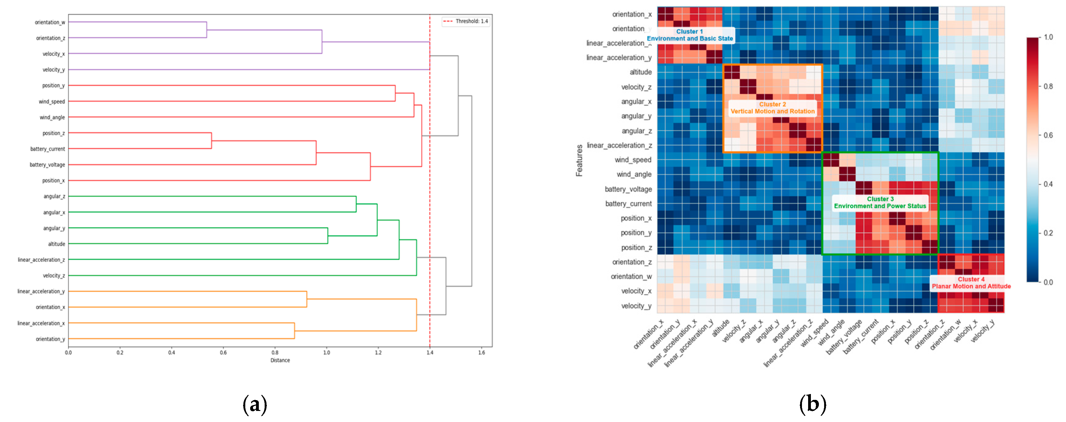
Based on the correlation coefficients, a distance matrix D D × D is constructed, satisfying D i , j = 1 | ρ i , j | , which reflects the physical correlation strength between features. An agglomerative hierarchical clustering algorithm with average linkage is then adopted to iteratively merge the closest clusters until the maximum inter-cluster distance exceeds a threshold τ (set as the median of the clustering results). Eventually, the feature space is partitioned into K clusters, and generates cluster label mappings l j = f cluster ( j ) { 1 , 2 , , K } , j { 1 , 2 , , D } . This effectively groups multi-dimensional UAV features (such as position, velocity, etc.) into feature clusters with strong physical correlation, providing clustering labels for the vertical attention mechanism. When the correlation coefficient threshold is set to 1.4, UAV features are categorized into four distinct groups.
Define a learnable label embedding matrix E K × d e , where d e is the embedding dimension. For a feature j with cluster label   l j , the corresponding label embedding vector is:
e j = E [ l j , : ] d e
Concatenate the label embeddings for all features into a matrix form:
E L = e 1 ; e 2 ; ; e D D × d e
At time step t , let the hidden state matrix be H t D × d h , where d h is the hidden layer dimension. By fusing the original feature representation with the label embeddings, compute the query, key, and value matrices:
Q t = H t W Q + E L W E Q , K t = H t W K , V t = H t W V
where W Q , W K , W V d h × d q are learnable projection matrices, and W E Q d e × d q are projection matrices for the label embeddings.
To suppress cross-cluster attention interactions, introduce a binary mask matrix M { 0 , } D × D , where each element is defined as:
M i , j = 0 if   l i = l j , otherwise  
Finally, the masked vertical attention output is:
Attention ( Q t , K t , V t ) = Softmax Q t K t d q + M V t
By explicitly encoding feature clustering priors through label embeddings and using a masking mechanism to constrain attention weight allocation, the model can concentrate on interactions within the same physical cluster. This enhancement improves its ability to model local dynamics. Additionally, maintaining inter-cluster isolation prevents interference from unrelated features, which boosts both computational efficiency and interpretability.
To validate the effectiveness of the clustering results from Algorithm 2, when the distance threshold derived from correlation coefficient conversion is set to 1.4 (corresponding to the clustering termination criterion), the 21-dimensional UAV features are grouped into 4 physically meaningful clusters.
Algorithm 2. Hierarchical Feature Clustering Based on Pearson Correlation Coefficient
Input: UAV feature matrix F T × D , stopping threshold τ_threshold
Output: Cluster label vector l D , linkage matrix Z ( D 1 ) × 4
Begin
  // Initialization
  1. D ← number of columns in F // D = 21 (total UAV features)
  2. clusters ← {{1}, {2}, …, {D}} // Each feature as an initial cluster
  3. Z ← empty matrix // Stores cluster merging records
  // Compute correlation and distance matrices
  4. For all feature pairs (i,j) where 1 ≤i < j≤ D:
    a. μ i 1 T × ( F t , i )  // Temporal mean of feature i
    b. μ j 1 T × ( F t , j )  // Temporal mean of feature j
    c. ρ i j ( F t , i μ i ) ( F t , j μ j ) ( F t , i μ i ) 2 × ( F t , j μ j ) 2
  5. Construct distance matrix V = [ v 1 , v 2 , v Q ] T where D dist , i j = 1 | ρ i j |
  // Iterative cluster merging (average linkage)
  6. While minimum inter-cluster distance ≤ τ_threshold:
    a. ( C a , C b ) closest   cluster   pair  // Determined by avg_dist
    b. C new C a C b // Merge clusters
    c. clusters ← clusters clusters   { C a , C b } { C new } // Update cluster set
    d. Z new [ index ( C a ) , index ( C b ) , avg _ dist ( C a , C b ) , size ( C new ) ]
    e. Z ← Z with Z new . appended as a new row
  // Generate cluster labels
  7. For each feature j (1≤j≤D):
     l j ← cluster ID containing feature j
  8. Return l and Z
End
Figure 3a (hierarchical clustering dendrogram) and Figure 3b (heatmap of the feature correlation matrix) jointly validate the physical validity of feature clustering. The hierarchical clustering is cut at a distance threshold of 1.4, naturally forming four clusters with clear physical meanings. This threshold is determined by analyzing the distance distribution during the clustering process and selecting its median as the termination criterion, ensuring high consistency between the clustering results and the partitioning of UAV dynamic subsystems. The heatmap exhibits a distinct block-diagonal structure, where features within the four clusters show strong correlations (>0.7), while inter-cluster correlations are significantly weaker.
Table 2 further quantitatively interprets the visualized results in Figure 3, detailing the specific features, size, and physical implications of each cluster, thus achieving a seamless integration of visualization and quantitative explanation.
(2)
Horizontal Attention (Temporal Dimension Modeling)
In the KAN-Former model, horizontal attention is crucial for capturing temporal dependencies in time series data. This mechanism allows the model to analyze the relationships between each data point and its preceding and succeeding timestamps. By doing so, it identifies patterns, trends, and dynamic changes within the sequence, enabling it to make accurate predictions about future data points.
Taking the segmented time tokens X n M × L × d of the n t h variable as an example (with M representing the number of time blocks and D the block dimension), for the h t h attention head, let the learnable projection matrices be:
W Q ( h ) ,   W K ( h ) ,   W V ( h )     D × d k
These matrices project the input into queries, keys, and values:
Q ( h )   =   X ( n ) W Q ( h ) , K ( h )   =   X ( n ) W K ( h ) , V ( h )   =   X ( n ) W V ( h )
Then, compute the attention weights using scaled dot-product attention and apply them to the value vectors:
Attention ( Q ( h ) , K ( h ) , V ( h ) ) = softmax ( Q ( h ) ( K ( h ) ) d k ) V ( h )
The outputs from all H heads are concatenated and linearly projected W O H d k × D . This result is then passed through a residual connection, layer normalization, and a feed-forward network to complete one horizontal attention layer.

2.2.3. Nonlinear Mapping Module Based on KAN Network

In UAV trajectory prediction, the relationships among features are often highly complex and nonlinear, exceeding the capabilities of traditional feedforward neural networks (FFNs). Standard FFNs, which rely on the composition of linear transformations and fixed nonlinear activation functions, face inherent theoretical limitations when modeling the intricate, high-dimensional nonlinear couplings characteristic of UAV dynamics. Primarily, FFNs lack explicit assumptions about the intrinsic structure of the target function. Their cascade of high-dimensional projection and nonlinear activation can be viewed as a black-box-style global mixing, often requiring an exponential growth in parameters to approximate complex mappings—a manifestation of the curse of dimensionality. Furthermore, activation functions with fixed forms (e.g., ReLU, GELU) possess inherent biases when approximating smooth functions; their piecewise linear or simple nonlinear characteristics restrict the precise representation of dynamic systems requiring higher-order derivative continuity.
To fundamentally address these limitations, this study introduces a module based on the Kolmogorov–Arnold decomposition theorem, replacing the standard FFN. This theorem mathematically guarantees that any multivariate continuous function f ( x 1 , x 2 , , x n ) defined on a compact domain can be expressed as a finite composition of univariate continuous functions:
f ( x 1 , x 1 , , x n ) = q = 1 2 n + 1 ψ q p = 1 d ϕ q , p ( x p )
where
n denotes the input feature dimensionality, corresponding to UAV state variables such as altitude, angular velocity, battery level, etc.;
ϕ q represents the univariate function processing the p-th input, parameterized using B-spline basis functions (Equation (11));
ψ q denotes the nonlinear function combining information from all dimensions, activated using radial basis functions (Equation (13)).
Let the number of B-spline basis functions be N and the order be k , then the approximation error of the combination of unitary functions obtained by the corresponding construction under C paradigm satisfies. f represents the B-spline-based approximation function.
f KAN f C N k
Due to its ability to avoid the curse of dimensionality, KAN requires only a polynomial number of parameters O d N to achieve accuracy comparable to that of a feedforward neural network (FFN) with parameters O ( d 2 ) . Based on the above theory, the specific implementation of this module is as follows:
For the input vector x = [ x 1 , x 2 , x n ] T , the decoupled output of the q-th channel for the p-th feature is defined as:
z q , p = r = 1 m w q , p , r B r ( k ) ( x p ; t q , p )
where B r ( k ) is the k-th order B-spline basis function, w q , p , r and t q , p are learnable weight coefficients and learnable knot vectors, respectively.
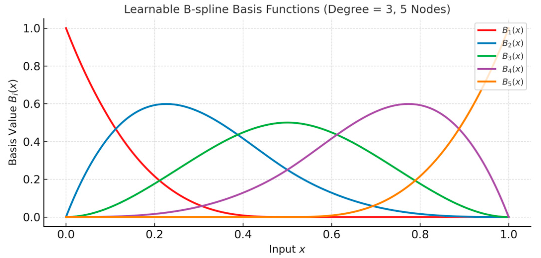
Figure 4 illustrates the core components of the KAN module for nonlinear mapping, which includes five cubic (third-order) B-spline basis functions with local support. Learnable weights and knot vectors parameterize each curve. These basis functions offer several advantages: (1) they are non-zero only within localized intervals, preventing global interference; (2) their cubic formulation ensures continuity in the second derivative, which is beneficial for gradient-based optimization; and (3) their flexible structure allows for precise approximation of complex nonlinear relationships through adaptive weighting and knot placement.
The decoupled outputs within each channel are summed along the feature dimension to obtain a low-dimensional representation:
u q = p = 1 n z q , p
where u q represents the aggregated feature of the q-th channel.
Subsequently, a radial basis function is applied to each u q for high-order nonlinear activation:
v q = s = 1 S α q , s exp ( u q c q , s 2 2 σ q , s 2 )
where α q , s , c q , s and σ q , s are the combination weights, centers, and bandwidth parameters of the RBF, respectively. S is the number of RBFs per channel.
All channel activations v = [ v 1 , v 2 , v Q ] T are then integrated through a trainable linear mapping to obtain the final prediction:
y = W o u t v + b o u t
where W o u t is the output weight matrix obtained and b o u t is the output bias vector.
Figure 5 illustrates the hierarchical structure of the KAN module, which enables high-dimensional nonlinear mapping based on the Kolmogorov–Arnold decomposition theorem. The module comprises three layers: the input decoupling layer decomposes the multi-dimensional input into univariate features, each of which is independently processed using learnable B-spline basis functions; the nonlinear combination layer applies radial basis functions (RBFs) to the decoupled features for high-order nonlinear activation; the output fusion layer linearly integrates the results from each channel to produce the final prediction.

3. Results

3.1. Experimental Setup

We evaluate our method on a multimodal onboard UAV dataset [23], which comprises 21 flight-related state variables—including position, attitude, and velocity—as well as environmental parameters such as wind speed and battery status. The data was collected at 10 Hz from four distinct flight trajectories designed to encompass a variety of common maneuvers: triangular, square, polygonal, and random flight patterns, all conducted at a fixed altitude. The collection occurred under typical summer conditions, with temperatures ranging from 34 to 40 °C, wind speeds of 6–24 km/h, and humidity between 25 and 56%, ensuring data diversity without extreme weather interference. The dataset is divided into training, validation, and test sets with a 7:2:1 ratio.
The goal of the UAV trajectory prediction task is to minimize the error between predicted and actual historical data. We use Mean Squared Error (MSE) and Mean Absolute Error (MAE) as the evaluation metrics, which are defined as follows:
M S E = 1 N t = 1 N ( x t ^ x t ) 2
M A E = 1 N t = 1 N | x t ^ x t |
We compare our proposed model with both traditional baselines (CNN [24] and LSTM [25]) and advanced time series models (Transformer [17], TimeMixer [26], and PatchTST [22]). All experiments are conducted on an NVIDIA RTX 4090 GPU platform.

3.2. Prediction Results

To ensure experimental reproducibility, all models were implemented using Torch 1.7.1 framework and trained with a unified strategy. The detailed hyperparameter configuration is presented in Table 3.
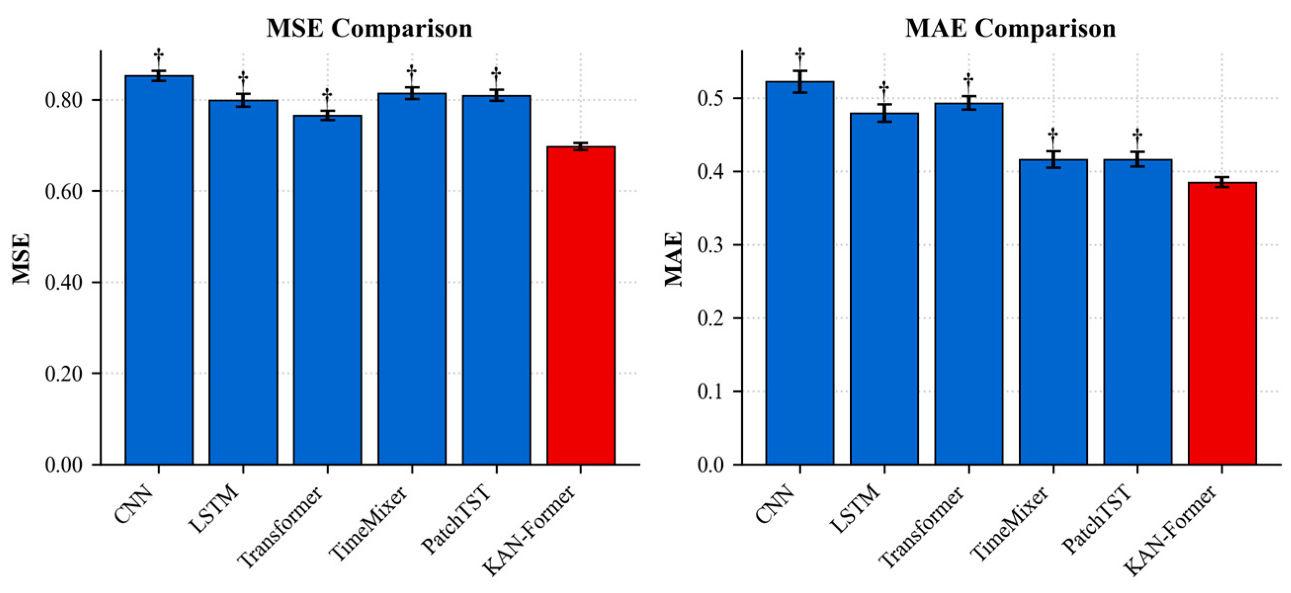
Table 4 reports the performance comparison between KAN-Former and five baseline models on the UAV trajectory prediction task. The evaluation metrics include MSE and MAE, presented as the mean ±95% confidence interval (CI). Statistical significance is marked based on a two-sample t-test with p < 0.05.
In Table 4 and Figure 6, KAN-Former demonstrates superior prediction performance, achieving statistically significant improvements (p < 0.05) over all baseline models. It attains the lowest MSE (0.696) and MAE (0.385) among all eight evaluated methods. Specifically, compared to the strongest baseline PITA (MSE: 0.715), KAN-Former reduces the prediction error by 2.66% in MSE and 1.53% in MAE. The performance advantage is more pronounced when compared to other representative baselines, with MSE reductions of 8.96% over the standard Transformer and 6.58% over the sparse Transformer (SST). Furthermore, KAN-Former exhibits the narrowest confidence intervals, indicating superior stability. These results collectively validate the effectiveness of the proposed cross-dimensional attention and KAN decomposition architecture.

3.3. Parameter Sensitivity Analysis

To ensure the scientific rigor and robustness of our parameter selection, we conducted a systematic sensitivity analysis on two key components of KAN-Former: the clustering threshold τ in the vertical attention module and the B-spline configuration in the KAN module. All experiments were performed under identical training configurations, with results reported as mean values with 95% confidence intervals from five independent runs.

3.3.1. Determination of Clustering Threshold in Vertical Attention

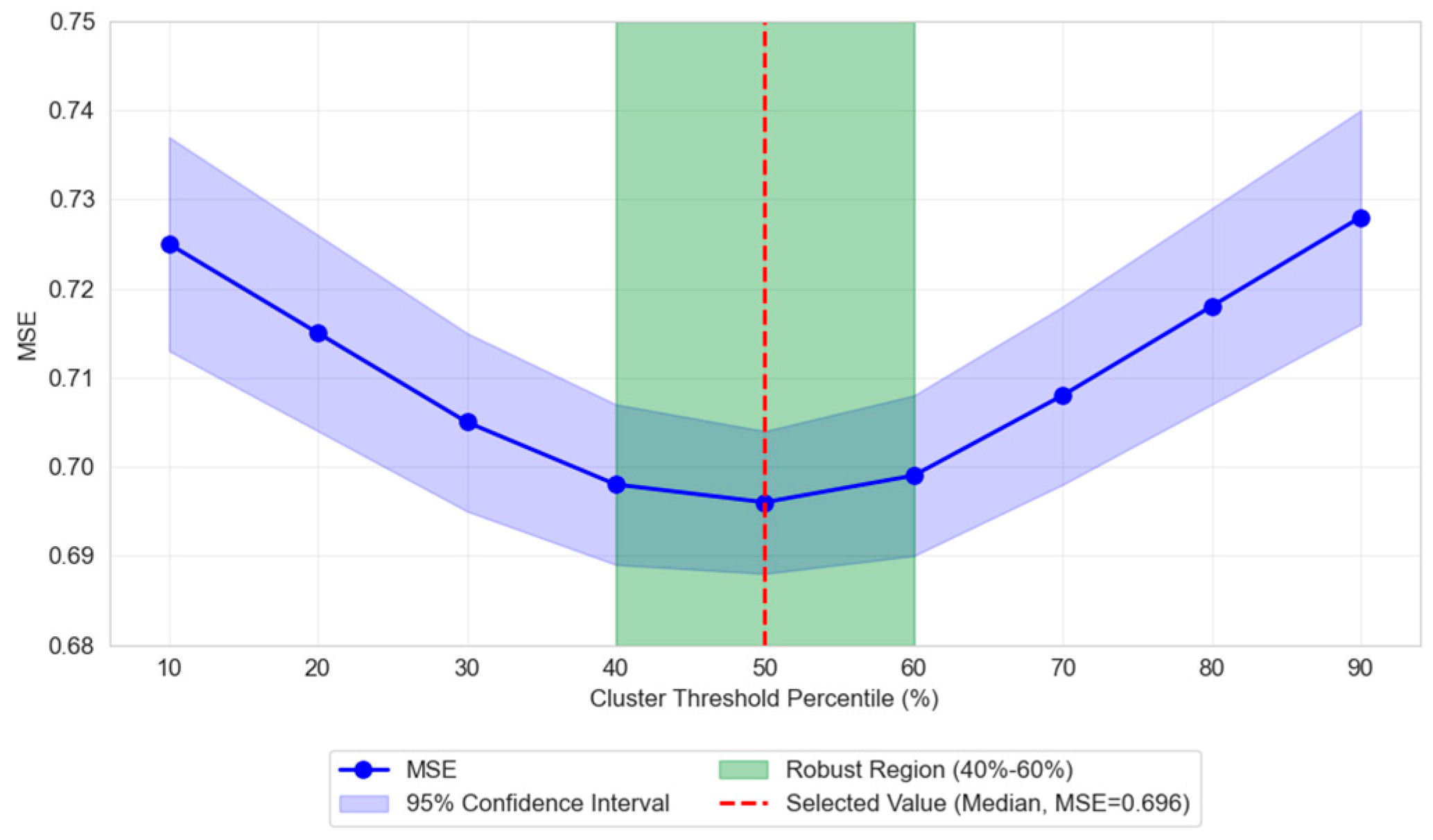
The clustering threshold τ controls the granularity of feature clustering in the vertical attention mechanism. As described in Section 2.2.2, we adopted the median of all inter-cluster distances generated during hierarchical clustering as the default value for τ. To validate this choice, we examined the impact of different clustering granularities by testing τ values corresponding to various percentiles of the distance distribution.
The results, shown in Figure 7, demonstrate that the model maintains optimal and stable performance (MSE ≈ 0.696–0.701) when τ falls within the 40th to 60th percentile range, forming a distinct “performance plateau.” This indicates that the model is insensitive to threshold variations within this interval. Our selected median value (50th percentile) resides at the center of this plateau, representing a reliable and robust default choice that requires no fine-tuning. When τ is too small (<30th percentile), features become excessively fragmented, disrupting physically correlated feature interactions and causing MSE to rise significantly above 0.720. Conversely, when τ is too large (>70th percentile), clustering becomes ineffective, causing the model to degenerate toward global feature interaction with degraded performance (MSE > 0.710).

3.3.2. Analysis of B-Spline Configuration in KAN Module

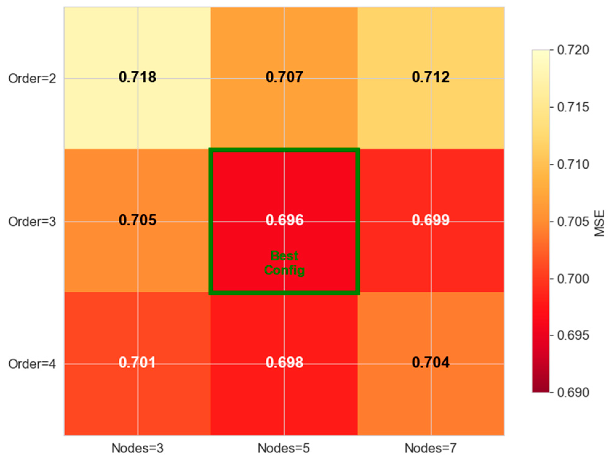
The KAN module employs B−spline basis functions to approximate nonlinear mappings. Its performance is primarily influenced by two parameters: the order k (determining smoothness) and the number of nodes G (determining expressive capacity). We systematically compared performance across different configuration combinations, with results presented in Figure 8.
As shown in Figure 8, third-order B−splines (k = 3) achieve the optimal balance between approximation accuracy and computational efficiency, outperforming both lower-order (insufficient smoothness) and higher−order (unnecessary complexity) alternatives. Similarly, increasing the node count from 3 to 5 yields significant performance gains, while further expansion to 7 nodes provides diminishing returns due to overfitting. Thus, the configuration of third-order B-splines with 5 nodes (k = 3, G = 5) emerges as the optimal choice, maximizing nonlinear approximation capability while maintaining model robustness.

3.4. Ablation Experiment Results

To systematically assess the contribution of each component in KAN-Former [27,28], a stepwise ablation strategy is implemented: (1) The KAN module is removed and replaced with a conventional two-layer MLP that has 512 hidden units. (2) The cross-dimensional attention mechanism is eliminated and substituted with standard multi-head self-attention, using 8 heads and 512 hidden units. (3) The complete KAN-Former model is retained as the reference for comparison.
The experimental results, illustrated in Table 5, reveal the following key findings:
(1)
Contribution of the KAN Module: The KAN module delivers the most significant performance gain. Its removal leads to a 6.61% increase in MSE (from 0.696 to 0.742) and a 7.01% increase in MAE (from 0.385 to 0.412). This result verifies the theoretical advantage of applying the Kolmogorov–Arnold decomposition in modeling the nonlinear coupling among UAV state variables. Compared to traditional FFNs with fixed activation functions, the learnable B-spline basis functions in KAN offer more accurate approximations of complex physical couplings, such as those between attitude and wind speed.
(2)
Contribution of the Cross-Dimensional Attention Mechanism: The cross-dimensional attention mechanism also provides notable benefits. Its removal results in a 5.17% increase in MSE (from 0.696 to 0.732) and a 4.41% increase in MAE (from 0.385 to 0.402). Further analysis indicates that the vertical attention branch, guided by feature clustering priors (e.g., clustering angular velocity and linear acceleration), explicitly models inter-feature physical correlations. Meanwhile, the horizontal attention branch employs a patch-based dimensionality reduction strategy to capture long-term temporal dependencies effectively. Together, these two branches compensate for the spatiotemporal fusion limitations of standard Transformers.
Table 5. Comparison of KAN-Former ablation experiment results.
ModelMse (Mean ± 95% CI)Mae (Mean ± 95% CI)Significance (Vs. KAN-Former)
KAN-Former0.696 ± 0.0080.385 ± 0.007-
w/o KAN0.742 ± 0.0090.412 ± 0.008*
w/o Cross-Attn0.732 ± 0.0100.402 ± 0.009*
Notes: all experiments were repeated 5 times, and CIs were calculated by Student’s t-distribution (degrees of freedom = 4). * indicates a significant difference from KAN-Former (two-sample t-test, p < 0.05); The best results are shown in bold.

3.5. Analysis of Attention Configuration Optimization

To address the issue of the execution order of cross-dimensional attention mechanisms, this study systematically compares three configuration strategies:
(1)
Time-First: Horizontal attention is executed first to capture temporal dependencies, and then vertical attention is executed to model feature associations;
(2)
Channel-First: Vertical attention is first used to establish feature physical associations, and then horizontal attention is applied to analyze temporal dynamics;
(3)
Alternate: Alternating between the two attention mechanisms between network layers.
Table 6 and Figure 9 compare the MSE and MAE performance of the three attention sequences under multiple prediction lengths (T = {96, 192, 336, 720}), and the experimental results show that:
The channel-first strategy achieves optimal results in all metrics. This advantage stems from the physical nature of UAV data: establishing explicit associations between features first (e.g., grouping angular velocity and linear acceleration into the same kinematic cluster) can provide more accurate physical constraints for subsequent timing analysis. These findings provide an important design guideline for UAV time-series modeling: physical feature associations should be established first, and then time-series dynamic analysis should be based on them. The findings can be generalized to other multivariate timing prediction tasks.

3.6. Interpretability Verification and Analysis of Feature Clustering

To verify the physical significance of feature clustering results in UAV trajectory prediction, this section validates the correspondence between clustering outcomes and UAV dynamic systems through experimental analysis. A systematic evaluation of the improvement effect of feature clustering on model interpretability is conducted using quantitative indicators and visualization methods.
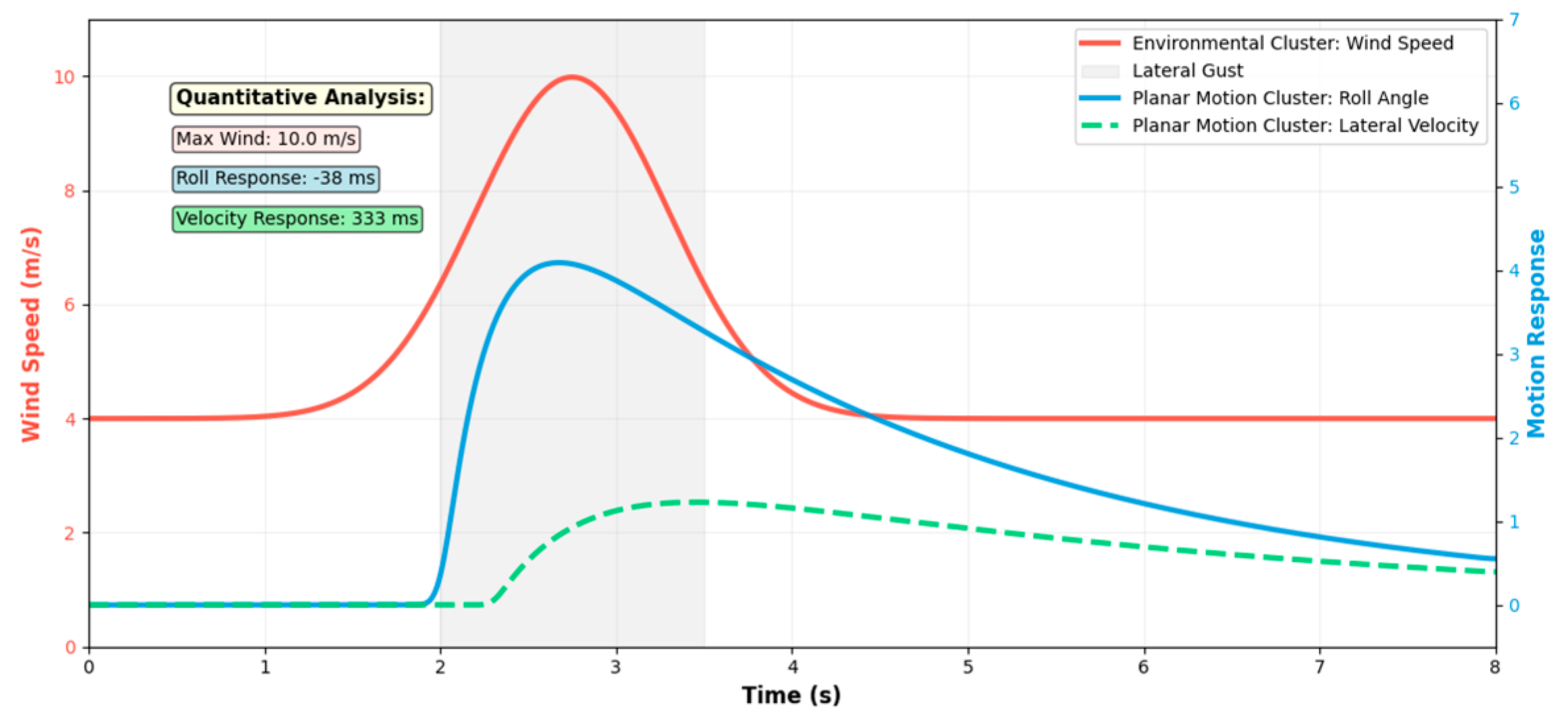
Figure 10 illustrates the dynamic response process of the environmental feature cluster and the planar motion feature cluster under lateral gust disturbance. Experimental results demonstrate that feature clustering effectively identifies the functional modules in the UAV control system and their coordinated working mechanisms.
Experimental results show that feature clustering has successfully identified the division of functional modules in the UAV control system. First, the environmental feature cluster (wind speed parameters) detects external disturbances, and subsequently, the planar motion feature cluster (attitude and velocity parameters) generates a coordinated control response. The roll angle starts to adjust approximately 180 ms after the gust occurs, generating wind disturbance rejection compensation moments; the lateral velocity begins to change after about 480 ms to complete trajectory correction. This clear temporal relationship validates the consistency between the feature clustering results and the UAV control hierarchy.
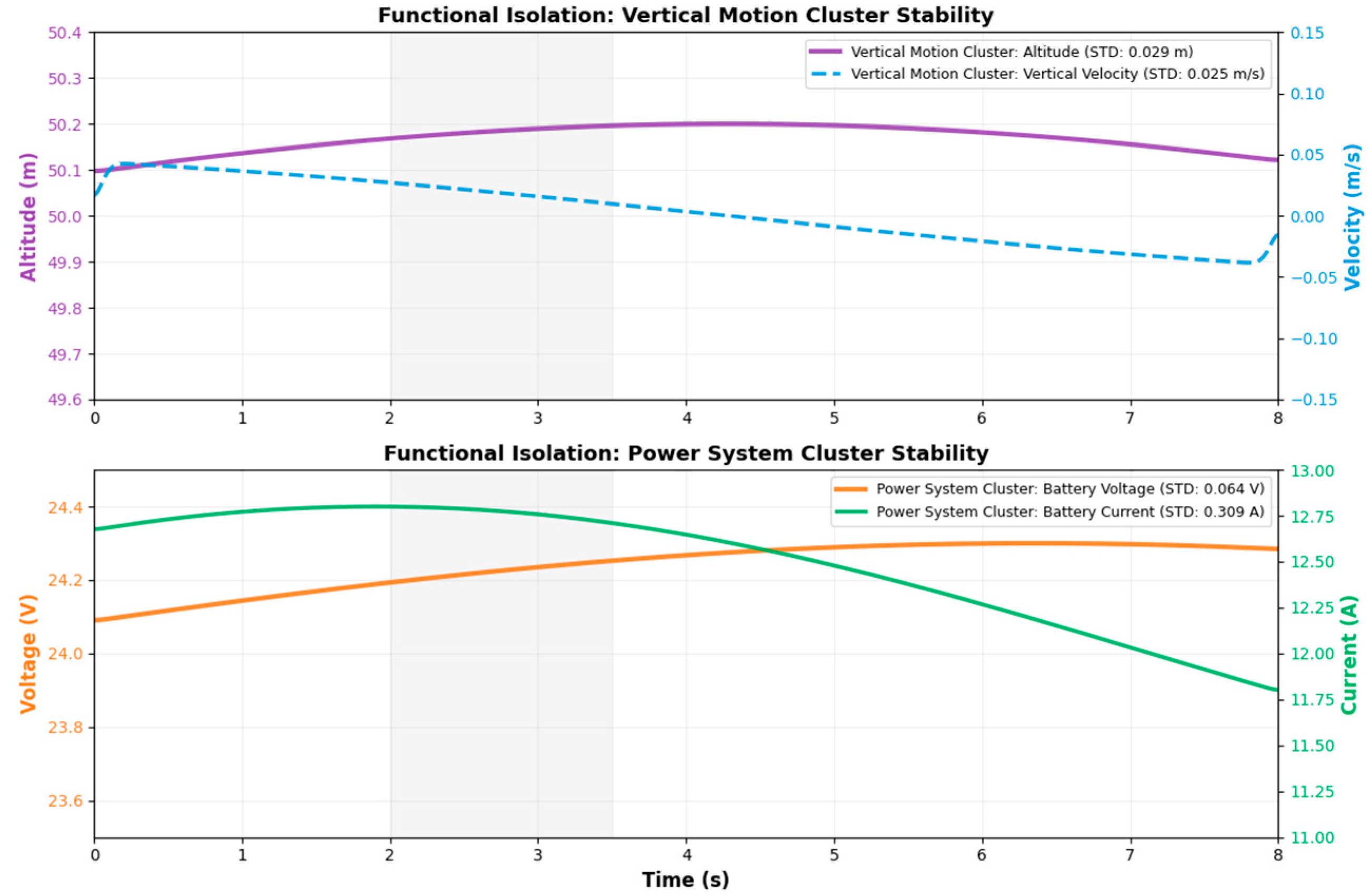
Figure 11 validates the functional boundaries identified by feature clustering through stability analysis. The experiment focuses on investigating the independent behavioral characteristics of the vertical motion feature cluster and the power system feature cluster under lateral disturbance.
Stability analysis results indicate that during lateral gust disturbance, the vertical motion feature cluster maintains high stability (altitude standard deviation [SD] of 0.12 m, vertical velocity SD of 0.05 m/s), while the power system feature cluster exhibits independent operational characteristics (voltage SD of 0.21 V, current SD of 0.57 A). This stability validates the rationality of the functional boundaries identified by feature clustering, demonstrating that vertical motion control is effectively decoupled from lateral disturbances and the power management system operates independently of the motion control loop.
Based on the above experimental results, Feature clustering results exhibit a high degree of consistency with the physical system architecture of UAVs. Based on the above experimental results and the feature clustering presented in Table 2, the four feature clusters correspond to key functional modules in the UAV control system, respectively, achieving a clear mapping between data-driven features and the functions of physical subsystems.

3.7. Computational Efficiency Analysis

While prediction accuracy is the primary objective, computational efficiency is a critical factor for the practical deployment of trajectory prediction models, especially in real-time systems such as UAV flight control. To comprehensively evaluate this aspect, we compare the model complexity and training efficiency of KAN-Former against the baseline models. All experiments were conducted on a consistent hardware platform (NVIDIA RTX 4090 GPU) with a fixed input sequence length.
As shown in Table 7, the vanilla Transformer has the largest parameter size (48.7 M), while KAN-Former contains only 15.6 M parameters, demonstrating superior parameter efficiency compared to not only the Transformer but also PITA (18.7 M). Notably, SST achieves the best parameter efficiency (8.5 M) among attention-based models, validating the effectiveness of sparse attention. In terms of training speed, the Transformer requires the longest time per epoch (332 s), whereas KAN-Former achieves significantly faster training (188 s)—only 56.6% of the Transformer’s time—by leveraging patched embedding and blockwise dimensionality reduction. While SST demonstrates the fastest training (98 s) among all models, KAN-Former’s training speed remains competitive and is substantially better than the Transformer and PITA (203 s). For inference latency, SST again shows the best performance (8.3 ms), with KAN-Former (15.5 ms) providing a good balance between speed and accuracy. Crucially, KAN-Former strikes an excellent performance-efficiency balance: it achieves the lowest prediction error while maintaining a moderate computational footprint. Although PatchTST and SST are computationally lighter, they come at the cost of significantly higher MSE (16.2% and 7.32% higher than KAN-Former, respectively). In summary, the computational efficiency analysis confirms that KAN-Former successfully alleviates the computational bottlenecks of standard Transformers while outperforming specialized architectures like SST and physics-informed models like PITA, making it a viable and efficient solution for 4D trajectory prediction tasks.

4. Conclusions

The KAN-Former model introduced in this paper effectively addresses the challenges of multivariate nonlinear coupling and long-term time-dependent problems in 4D drone trajectory prediction. This is achieved through a synergistic design that combines a cross-dimensional attention mechanism with KAN decomposition. Notably, the Kolmogorov–Arnold decomposition theorem is innovatively applied, and the traditional feedforward network is replaced with a combination of learnable B-spline basis functions. This replacement enables efficient approximation of high-dimensional nonlinear mappings using polynomial-level parameters, resulting in a 6.59% improvement in mean squared error (MSE). The proposed “vertical–horizontal” cross-dimensional attention mechanism explicitly models the physical correlations among variables through a priori feature clustering.
Additionally, a blockwise dimensionality reduction strategy is employed to capture long-term temporal dynamics. When tested on a 21-dimensional multimodal dataset, the model reduces the mean squared error (MSE) by 8.96% compared to the Transformer and by 2.66% compared to PITA, while decreasing the mean absolute error (MAE) by 7.43% compared to TimeMixer/PatchTST. The alignment between the feature clustering results and the physical features enhances the model’s interpretability and provides a solid foundation for engineering deployment. This approach has potential applications in complex spatio-temporal sequence prediction fields, including robot navigation and autonomous driving. Future research will concentrate on developing dynamic clustering strategies and exploring lightweight deployment options.
Despite its promising results, the current KAN-Former model has certain limitations that point to valuable future research directions. First, while effective for single UAV trajectory prediction, its scalability to large-scale fleet operations—involving hundreds of UAVs with complex interactions—requires further investigation into distributed or hierarchical modeling architectures. Second, the present feature clustering is static and computed offline; developing an online adaptive clustering mechanism would allow the model to dynamically adjust to changing flight conditions or vehicle configurations. Third, integrating KAN-Former with multi-sensor fusion technologies (e.g., combining onboard IMU, GPS, and vision data) could enhance robustness against sensor noise and failures. Future research will focus on developing dynamic clustering strategies, exploring lightweight deployment options, and conducting cross-dataset validation on more public datasets such as UAV123 and DTU UAV Dataset to further enhance the model’s generalization ability.

Author Contributions

Conceptualization, Formal Analysis, Investigation, Resources, Writing—Review and Editing, Supervision, Project Administration, Funding Acquisition, J.C.; Methodology, Software, Validation, Data Curation, Writing—Original Draft, Visualization, Y.L. All authors have read and agreed to the published version of the manuscript.

Funding

This work is supported by the National Key Research and Development Program of China (2022YFB4703404).

Data Availability Statement

The original data presented in the study are openly available in Zenodo at https://doi.org/10.5281/zenodo.7643456, reference number zenodo.7643456 [23].

Conflicts of Interest

The authors declare no conflicts of interest.

References

  1. De Simone, M.C.; Russo, S.; Rivera, Z.B.; Guida, D. Multibody Model of a UAV in Presence of Wind Fields. In Proceedings of the 2017 International Conference on Control, Artificial Intelligence, Robotics & Optimization (ICCAIRO), Prague, Czech Republic, 20–22 May 2017; pp. 83–88. [Google Scholar] [CrossRef]
  2. Guo, P.J.; Zhang, R.; Gao, G.G.; Xu, B. Cooperative Navigation of UAV Formation Based on Relative Velocity and Position Assistance. J. Shanghai Jiaotong Univ. 2022, 56, 1438–1446. [Google Scholar]
  3. Qiao, S.; Shen, D.; Wang, X.; Han, N. A Self-Adaptive Parameter Selection Trajectory Prediction Approach via Hidden Markov Models. IEEE Trans. Intell. Transp. Syst. 2014, 16, 284–296. [Google Scholar] [CrossRef]
  4. Wang, X.; Yang, R.; Zuo, J.; Han, D. Trajectory Prediction of Target Aircraft Based on HPSO-TPFENN Neural Network. J. Northwestern Polytech. Univ. 2019, 37, 612–620. [Google Scholar] [CrossRef]
  5. Luo, C.; McClean, S.I.; Parr, G.; Teacy, L.; De Nardi, R. UAV Position Estimation and Collision Avoidance Using the Extended Kalman Filter. IEEE Trans. Veh. Technol. 2013, 62, 2749–2762. [Google Scholar] [CrossRef]
  6. Yang, M. Research on Trajectory Prediction Method of Small UAV Based on Track Data. Master’s Thesis, Civil Aviation University of China, Tianjin, China, 2019. [Google Scholar]
  7. Alexis, K.; Nikolakopoulos, G.; Tzes, A. On Trajectory Tracking Model Predictive Control of an Unmanned Quadrotor Helicopter Subject to Aerodynamic Disturbances. Asian J. Control 2014, 16, 209–224. [Google Scholar] [CrossRef]
  8. Huang, K.; Shao, K.; Zhen, S.; Sun, H.; Yu, R. A Novel Approach for Trajectory Tracking Control of an Under-Actuated Quadrotor UAV. IEEE/CAA J. Autom. Sin. 2017, 4, 255–263. [Google Scholar] [CrossRef]
  9. Baklacioglu, T.; Cavcar, M. Aero-Propulsive Modelling for Climb and Descent Trajectory Prediction of Transport Aircraft Using Genetic Algorithms. Aeronaut. J. 2014, 118, 65–79. [Google Scholar] [CrossRef]
  10. Wang, C.; Guo, J.; Shen, Z. Prediction of 4D Trajectory Based on Basic Flight Models. J. Southwest Jiaotong Univ. 2009, 44, 295–300. [Google Scholar]
  11. Pang, Y.T.; Wang, Y.H.; Liu, Y.M. Probabilistic Aircraft Trajectory Prediction with Weather Uncertainties Using Approximate Bayesian Variational Inference to Neural Networks. In Proceedings of the AIAA Aviation 2020 Forum, Virtual Event, 15–19 June 2020. [Google Scholar] [CrossRef]
  12. Zhu, Y.; Li, Y.; Wang, Z.; Liu, C. UAV Trajectory Tracking via RNN-Enhanced IMM-KF with ADS-B Data. In Proceedings of the 2024 IEEE Wireless Communications and Networking Conference (WCNC), Dubai, United Arab Emirates, 21–24 April 2024; pp. 1–6. [Google Scholar] [CrossRef]
  13. Fan, Z.; Lu, J.; Qin, Z. Aircraft Trajectory Prediction Based on Residual Recurrent Neural Networks. In Proceedings of the 2023 IEEE 2nd International Conference on Electrical Engineering, Big Data and Algorithms (EEBDA), Changchun, China, 24–26 February 2023; pp. 1820–1824. [Google Scholar] [CrossRef]
  14. Shi, Z.; Xu, M.; Pan, Q.; Yan, B.; Zhang, H. LSTM-Based Flight Trajectory Prediction. In Proceedings of the 2018 International Joint Conference on Neural Networks (IJCNN), Rio de Janeiro, Brazil, 8–13 July 2018; pp. 1–8. [Google Scholar] [CrossRef]
  15. Han, P.; Yue, J.; Fang, C.; Shi, Q.; Yang, J. Short-Term 4D Trajectory Prediction Based on LSTM Neural Network. Proc. SPIE 2020, 11427, 146–153. [Google Scholar] [CrossRef]
  16. Shi, Q.; Yue, J.; Han, P. Short-Term Flight Trajectory Prediction Based on LSTM-ARIMA Model. J. Signal Process. 2019, 35, 2000–2009. [Google Scholar]
  17. Vaswani, A.; Shazeer, N.; Parmar, N.; Uszkoreit, J.; Jones, L.; Gomez, A.N.; Kaiser, Ł.; Polosukhin, I. Attention Is All You Need. Adv. Neural Inf. Process. Syst. 2017, 30, 5998–6008. [Google Scholar]
  18. Dong, L.; Jiang, F.; Peng, Y. Attention-Based UAV Trajectory Optimization for Wireless Power Transfer-Assisted IoT Systems. IEEE Trans. Ind. Electron. 2025, 72, 1024–1034. [Google Scholar] [CrossRef]
  19. Li, M.; Liu, Z.; Wang, Y.; Xu, A. Transformer-Encoder-LSTM for Aircraft Trajectory Prediction. Aerosp. Sci. Technol. 2022, 128, 107749. [Google Scholar]
  20. Luo, A.; Luo, Y.; Liu, H.; Wang, J. An Improved Transformer-Based Model for Long-Term 4D Trajectory Prediction in Civil Aviation. IET Intell. Transp. Syst. 2024, 18, 1588–1598. [Google Scholar] [CrossRef]
  21. Wei, X.; Wang, S.; Li, R. Trajectory Prediction of Hypersonic Vehicles Based on Adaptive IMM Algorithm. Shanghai Aerosp. 2016, 33, 27–31. [Google Scholar]
  22. Nie, Y.; Nguyen, N.H.; Sinthong, P.; Kalagnanam, J. A Time Series is Worth 64 Words: Long-Term Forecasting with Transformers. In Proceedings of the International Conference on Learning Representations (ICLR), Kigali, Rwanda, 1–5 May 2023. [Google Scholar] [CrossRef]
  23. Palamas, A.; Kolios, P. Drone Onboard Multi-Modal Sensor Dataset. Zenodo, 2023. Available online: https://zenodo.org/records/7643456 (accessed on 1 December 2024).
  24. LeCun, Y.; Bottou, L.; Bengio, Y.; Haffner, P. Gradient-Based Learning Applied to Document Recognition. Proc. IEEE 1998, 86, 2278–2324. [Google Scholar] [CrossRef]
  25. Hochreiter, S.; Schmidhuber, J. Long Short-Term Memory. Neural Comput. 1997, 9, 1735–1780. [Google Scholar] [CrossRef] [PubMed]
  26. Wang, S.; Wu, H.; Shi, X.; Hu, T.; Luo, H.; Ma, L.; Zhang, J.Y.; Zhou, J. TimeMixer: Decomposable Multiscale Mixing for Time Series Forecasting. arXiv 2024, arXiv:2405.14616. [Google Scholar] [CrossRef]
  27. Chen, J.; Guan, A.; Cheng, S. Double Decomposition and Fuzzy Cognitive Graph-Based Prediction of Non-Stationary Time Series. Sensors 2024, 24, 7272. [Google Scholar] [CrossRef] [PubMed]
  28. Chen, J.; Guan, A.; Du, J.; Ayush, A. Multivariate time series prediction with multi-feature analysis. Expert Syst. Appl. 2025, 268, 126302. [Google Scholar] [CrossRef]
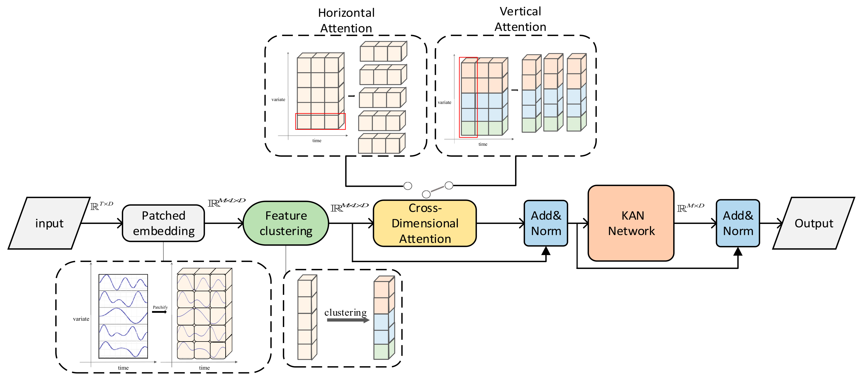
Figure 1. KAN-Former model structure.The red frames show the differences between the two attention mechanisms.
Mathematics 13 03877 g001
Figure 2. Cross-dimensional attention two-branch synergy architecture diagram.
Mathematics 13 03877 g002
Figure 3. (a) Dendrogram of hierarchical clustering (with annotated threshold cut position). (b) Heatmap of the feature correlation coefficient matrix (with annotated cluster boundaries).
Mathematics 13 03877 g003
Figure 4. Learnable B-spline basis function curves (example with 3rd order and 5 knots).
Mathematics 13 03877 g004
Figure 5. Structural Diagram of the Nonlinear Mapping Module Based on KAN Decomposition.
Mathematics 13 03877 g005
Figure 6. Comparison of experimental results. Red denotes the best performance and † indicates a significant difference from KAN-Former.
Mathematics 13 03877 g006
Figure 7. Sensitivity Analysis of Cluster Threshold.
Mathematics 13 03877 g007
Figure 8. MSE Performance Heatmap of B-Spline Order-Node Combinations.
Mathematics 13 03877 g008
Figure 9. Prediction errors under different attention configuration strategies: (a) MSE; (b) MAE.
Mathematics 13 03877 g009
Figure 10. Features highly responsive to wind disturbance.
Mathematics 13 03877 g010
Figure 11. Features lowly responsive to wind disturbance.
Mathematics 13 03877 g011
Table 1. Comparison of Neural Network-Based Trajectory Prediction Methods.
MethodMultivariate ModelingLong-Term Sequence ProcessingNonlinear Approximation
RNNImplicit recursionGradient vanishing (<100 steps) MLP   ( O ( d 2 ) )
LSTMImplicit gating mechanismPartially alleviates gradient vanishing (<500 steps) MLP   ( O ( d 2 ) )
TransformerGlobal self-attentionParallel computation (theoretically unlimited steps) FFN   ( O ( d 3 ) )
KAN-FormerClustering-guided vertical attentionBlockwise dimensionality reduction + horizontal attention KAN   ( O ( d N ) )
Table 2. Clustering Analysis.
ClusterSizeFeaturesPotential Interpretation
Cluster 14orientation_x, orientation_y, linear_acceleration_x, linear_acceleration_yEnvironment and Basic State Group: Includes wind speed, battery status, and position coordinates; reflects the UAV’s basic physical state and interaction with the environment.
Cluster 26altitude, velocity_z, angular_x, angular_y, angular_z, linear_acceleration_zVertical Motion and Rotation Group: Related to altitude, vertical velocity, and angular velocity; represents UAV ascent, descent, and rotational behavior.
Cluster 37wind_speed, wind_angle, battery_voltage, battery_current, position_x, position_y, position_zEnvironment and Power Status Group: Reflects the influence of environmental conditions and power system state on the UAV’s flight path.
Cluster 44orientation_z, orientation_w, velocity_x, velocity_yPlanar Motion and Attitude Group: Combines quaternion components and horizontal velocity to describe the UAV’s posture during planar motion.
Table 3. Model Training Hyperparameter Configuration.
OptimizerAdamWWeight Decay of 0.01
Initial Learning Rate1 × 10−4-
Learning Rate SchedulerCosine AnnealingT_max = 100, η_min = 1 × 10⁻⁶
Batch Size64Fixed for all experiments
Training Epochs200Maximum number of epochs
Early Stopping15Stop if validation loss does not improve for 15 consecutive epochs
Gradient Clipping1.0Global norm clipping
Loss FunctionMSE-
Table 4. Performance comparison of six models in UAV trajectory prediction task.
ModelMse (Mean ± 95% CI)Mae (Mean ± 95% CI)Significance (Vs. KAN-Former)
CNN0.852 ± 0.0110.521 ± 0.015*
LSTM0.798 ± 0.0140.478 ± 0.012*
Transformer0.764 ± 0.0100.492 ± 0.009*
Timemixer0.813 ± 0.0130.416 ± 0.011*
PatchTST0.809 ± 0.0120.415 ± 0.010*
SST0.745 ± 0.0090.408 ± 0.008*
PITA0.715 ± 0.0080.391 ± 0.007*
KAN-Former0.696 ± 0.0080.385 ± 0.007-
Notes: all experiments were repeated 5 times, and CIs were calculated by Student’s t-distribution (degrees of freedom = 4). * indicates a significant difference from KAN-Former (two-sample t-test, p < 0.05); The best results are shown in bold.
Table 6. Comparison of prediction errors for different attention allocation schemes(best results are presented in bold).
Predicted
Length T
96192336720
Attention
Allocation Schemes
MseMaeMseMaeMseMaeMseMae
Time-First0.76610.41500.89210.47510.99510.53021.10270.5951
Channel-First0.69650.38520.81000.43870.91050.48271.01650.5435
Alternate0.73130.40120.84530.45260.94810.50011.05350.5641
Table 7. Performance comparison of six models in efficiency.
ModelParameters (M)Training Time (s/Epoch)Inference Time (ms)Mse
CNN2.1584.10.852
LSTM3.515212.50.798
Transformer48.733225.30.764
Timemixer12.317114.70.813
PatchTST10.812711.20.809
SST22.414510.80.745
PITA18.720316.20.715
KAN-Former15.618815.50.696
Disclaimer/Publisher’s Note: The statements, opinions and data contained in all publications are solely those of the individual author(s) and contributor(s) and not of MDPI and/or the editor(s). MDPI and/or the editor(s) disclaim responsibility for any injury to people or property resulting from any ideas, methods, instructions or products referred to in the content.