On the Aitken–Hotelling–Duncan Formula: Brief History, Direct Derivations, and Effective Conditioning

Abstract

In the first part of this paper, we examine historical documents related to the well-known Sherman–Morrison–Woodbury (SMW) formula and suggest that Aitken–Hotelling–Duncan (AHD) is an appropriate name for the same formula. In the second part, we present two elementary direct derivations of the formula, including a slow method that utilizes a QR trick and a fast method that makes the common practice of depending on being given an inverse formula for verification unnecessary. In the third part, we develop significant improvements over the classic conditioning bounds of Yip. Numerical experiments show that our bounds can be several orders of magnitude sharper than Yip’s bounds. Yip’s conditioning bounds suggest that numerical instability of the AHD formula may be common. However, for an important formula that has found and continues to find diverse applications, its numerical stability in general is not expected to be pessimistic. Our improved bounds shed a new light on the generally perceived tricky stability issue related to the AHD formula and provide clearer theoretical support for its stable performance observed by different researchers in diverse applications.

1. Introduction

For various historical reasons, what may have been called the Aitken–Hotelling–Duncan (AHD) formula has been dominantly known as the Sherman–Morrison–Woodbury (SMW) formula. The formula was discovered and rediscovered by different researchers, for example, by Duncan [1] and Guttman [2] in the mid-1940s, about five years earlier than Sherman–Morrison [3,4] and Woodbury [5]. Such a repeated discovery is a strong sign of the importance of the formula.

“An important formula is not easily laid to rest.” This quote is from Hager [6]; it aptly points out a golden criterion that can measure the magnitude of significance of a formula: How well does it endure the test of the relentless passing of time?

The AHD/SMW formula passes the test of time remarkably well. Instead of being laid to rest, it has thrived. Derivations of the formula and its variants have continued since the 1950s. Representative works include Henderson and Searle [7] and Hager [6]. One of the classic and powerful approach for the derivation is via the Schur complements (see, e.g., [7] and Bojock (p. 128, [8])). Strang presents a similarly powerful approach in (pp. 161–162, [9]) using block Gauss elimination.

More importantly, the AHD/SMW formula and its variants have continued to find new applications in diverse fields. For example, Kailath utilized the formula in his pioneering work [10] to prove the equivalence of the Winner filter and a maximum-likelihood process, while Brooks and Reed applied the formula to establish the equivalence of the Wiener filter and the maximum signal-to-noise ratio filter [11].

More recent applications include those in diverse fields such as: Google search engines [12]; recursive least squares (RLS) and Kalman filtering (e.g., [13,14,15,16]); wireless communications (e.g., [17]); dynamical systems (e.g., [18,19]); flow simulations (e.g., [20]); structured equations (e.g., [21,22,23]); and machine learning (e.g., [24,25,26,27]).

The AHD/SMW formula and its variants are known for their efficiency for inverting matrices of form $B\pm E$, where B is inexpensive to invert, and E is low rank (usually as a product of low-rank matrices). To emphasize the low-rank property in E, the $B\pm E$ structure is often called the low-rank perturbation in traditional fields, such as dynamical systems and control, and the low-rank update in machine learning. Such a structure arises frequently in diverse fields, and there is great demand for computing or approximating ${(B\pm E)}^{-1}$ efficiently. Representative demands include those from Gaussian processes (GPs) (p. 201, [28]) and reinforcement learning (RL) (Chapter 9, [29]). The formula is frequently utilized to exploit the low-rank updates naturally occurring to the kernel matrices in GP and the Bellman matrices in RL. Owing to such continual and progressive demands, the formula not only ages well but also shows renewed vigor in an age of machine learning and artificial intelligence.

For such an influential formula over 75 years old, it can be difficult to shed new lights on it since the vast existing literature usually implies that most of the important aspects of the formula have been covered. However, we find three topics that are still worth writing on.

First, in Section 2, we examine historical documents to argue that AHD is at least as equally deserving a name for the formula as SMW. In our opinion, AHD is a more appropriate name than SMW.

Second, in Section 3, we present two methods for the direct derivation that do not seem to exist in the literature, one slow and one fast. The slow method can clearly show the interconnections among related formulas; it also introduces a QR trick useful for conditioning bounds. The fast method can make the common practice of directly verifying a given inverse formula via matrix multiplications appear burdensome. The derivations in Section 3 are suitable for an advanced undergraduate course on linear algebra.

Lastly, in Section 4, we develop significant improvements over the classic conditioning bounds of Yip [30]. Numerical experiments show that our bounds can be several orders of magnitude sharper than the bounds in [30]. The QR trick that we use for the direct derivation of the formula in Section 3 plays a key role in the development of our conditioning bounds. Our improved bounds shed a new light on the generally perceived tricky stability issue related to the formula and provide theoretical support to the observations reported (e.g., in [18,19]) and other cases where the formula naturally performs stably.

A formula that passes the test of time and continues to find new applications in diverse fields necessitates a stability exceeding the bounds suggested in [30]. Our improved bounds theoretically justify this possibly long-held but less-articulated expectation.

2. Some Brief History

Two excellent reviews of Henderson and Searle [7] and Hager [6] contain scrupulous historical accounts of the development of related formulas predating Sherman–Morrison [3,4] and Woodbury [5].

Duncan [1] already contains the complete form of what is later called the Woodbury formula (or the SMW formula in general). In [1], Duncan particularly mentioned that “the expression for the reciprocal of a partitioned matrix which appears in Equation 3.3 has been given by Dr. A. C. Aitken of Edinburgh in lectures to his students, together with some alternative equivalent forms which are now included in the present paper.” We do not have access to the mentioned lecture notes, but it is reasonable to assume that Aitken’s notes were later included in his book [31].

In [1], Duncan also credited Hotelling [32] for developing related formulas.

Waugh in [33] improved Hotelling’s method for deriving the same formula by reducing four inversions of half-sized matrices into just two inversions.

Guttman [2] also contributed to the derivation of the formula, but he appeared unaware of Duncan’s [1] before submitting [2]. At the footnote on the first page of [2], he wrote that “Professor Harold Hotelling has called my attention to reference [1], which overlaps substantially with the present paper…”

Duncan in [1] also cited Frazer et al. [34]—a book on Elementary Matrices that he coauthored. This book [34] already contains techniques for obtaining the inverse of a $2\times 2$ block matrix (such a block matrix is called the “augmented”, “enlarged”, or “bordered” matrix by later researchers). The origin of the inverse formula of the augmented $2\times 2$ block matrix traces back to Banachiewicz [35,36] (as cited in [7]). Guttman in [2] termed the techniques using block-augmented matrices the enlargement principle. Both Duncan’s and Guttman’s derivations utilized this enlargement technique.

Henderson and Searle had a precise summary of Duncan [1] on page 56 of [7]. They in particular noted that Duncan [1] “does give (1), in what seems to be its first appearance.”

$$\begin{array}{c}\hfill {(A-U{D}^{-1}V)}^{-1}=A^{-1}+A^{-1}U{(D-V{A}^{-1}U)}^{-1}V{A}^{-1}.\end{array}$$

(1)

In (1), the A and D are invertible, of size $n\times n$ and $m\times m$, respectively, and U and V are of size $n\times m$ and $m\times n$, respectively. We note that (1) is already the modern form of what is known as the SMW formula, with the minor exception that the modern form often uses $V^T$ (or $V^H$ in the complex case) in place of V so that the U and V matrices can have the same dimensions.

Next, we take a closer look at some historical documents related to the Sherman–Morrison formula.

The formula commonly attributed to Sherman and Morrison based on [3,4] is

$$\begin{array}{c}\hfill {(A+u{v}^T)}^{-1}=A^{-1}-{\displaystyle \frac{A^{-1}u{v}^T{A}^{-1}}{1+v^T{A}^{-1}u}},\end{array}$$

(2)

where A is invertible and u and v are compatible vectors, with $1+v^T{A}^{-1}u\ne 0$.

The work [3] is a one-third-page abstract. It describes an algorithm instead of presenting a formula. This algorithm, as pointed out by Hager [6], contains typographic errors, which may stem from its complicated elementwise notation. The subsequent paper [4] also describes an algorithm rather than a compact formula.

Somewhat surprisingly, Formula (2) dominantly attributed to Sherman and Morrison is not contained in either [3] or [4].

The title of [3] says the inverse is for a matrix with changes in a row or in a column, while [4] is even more specific—the inverse is for a matrix with only one element changed. However, (2) is for the inverse of $A+u{v}^T$ in which the $u{v}^T$ may change all elements of A. More specifically, [3] is for $u=c{e}_i$ or $v=d{e}_j$, and [4] is for both $u=c{e}_i$ and $v=d{e}_j$, where $e_i$ and $e_j$ denote standard basis vectors, and c and d are nonzero scalars; both are special cases of (2). At the end of [4], Sherman and Morrison suggested “successive applications of the method” to address a matrix with changes in two or more elements. In contrast, (2) can address such multiple element changes in one-shot, which is more convenient than the “successive applications” suggested by Sherman and Morrison, especially when all elements in A got changed by $u{v}^T$.

Hager [6] traces Formula (2) back to Bartlett [37]. Indeed, Sherman and Morrison [3,4] are special cases of (2), and Bartlett explicitly stated that his formula “includes the cases considered by Sherman and Morrison” in the introduction part of [37].

Woodbury in [5] cited Bartlett [37] as “submitted for publication”, what he generalized is Bartlett’s (2) instead of the narrower but more complicated algorithms in [3,4].

On page 2 of [5], Woodbury wrote the following:

“Let A be a nonsingular $n\times n$ matrix, let S be a square $m\times m$ matrix and let U and V be $n\times m$ and $m\times n$ rectangular matrices, then

$$\begin{array}{c}\hfill {(A+U{S}^{-1}V)}^{-1}=A^{-1}-A^{-1}US{(S+SV{A}^{-1}US)}^{-1}SV{A}^{-1}.\end{array}$$

(3)

If further S is non-singular, then the equation

$$\begin{array}{c}\hfill {(A-U{S}^{-1}V)}^{-1}=A^{-1}+A^{-1}U{(S-V{A}^{-1}U)}^{-1}V{A}^{-1},\end{array}$$

(4)

holds.”

Comparing Woodbury’s (4) with the Formula (1) that already exists in Duncan [1], we see that they are identical (using S or D makes no difference to the formula).

Woodbury appeared to consider (3) as more general than (4) since he only assumed S to be invertible for (4) but not for (3). However, since S in (3) is a common factor in the invertible matrix $S+SV{A}^{-1}US$, this S must also be invertible, which makes (3) equivalent to (4), not more general.

Woodbury obtained (4) via inverting “bordered matrices”—the same technique used by Duncan in [1] and by Guttman in [2]. A notable difference is that Duncan derived the inverse formula of a $2\times 2$ bordered matrix in [1], while Woodbury directly specified the inverse of the bordered matrix and stated that “(the inverse) can be verified by multiplication” in [5].

The commonly adopted view is that Woodbury was unaware of the earlier work of Duncan et al., and in [5], he cited none of their work. However, from the fact that Woodbury did not seek a formal publication of [5], and it has remained a technical report since 1950, it is plausible that he became aware of the earlier work after finishing [5].

The above brief historical review shows that Sherman and Morrison [3,4] address only special cases of (2), and (2) itself is a special case of (4). However, (4) is already explicitly derived in [1], six years before Woodbury stated it in [5] without a derivation.

Owing to the fact that Duncan [1] already contains the explicit form of what is later called the SMW formula, and that Duncan in [1] credited the essential contributions of Aitken and Hotelling for the formula, we feel it is appropriate to call the SMW formula the Aitken–Hotelling–Duncan (AHD) formula.

There are similar situations in which initial inventors of certain theories (including formulas) do not receive the credits they deserve. Here, we list only three examples:

• As pointed out in (p. 1, [38]), the influential Kantorovich inequality is named after Kantorovich (1975 Nobel Laureate in Economy) based on his derivation in a survey paper published in Russian in 1948. (In matrix form, the inequality claims that for a (Hermitian) positive definite matrix A with eigenvalues inside the interval $[{\lambda }_1,{\lambda }_n]$, $x^{H}Ax{x}^H{A}^{-1}x\le {(x^{H}x)}^2{({\lambda }_1+{\lambda }_n)}^2/(4{\lambda }_1{\lambda }_n)$.) However, the inequality was already published five years earlier by graph theorist Frucht in Spanish in 1943.
• The FWL theorem (https://en.wikipedia.org/wiki/Frisch-Waugh-Lovell_theorem, accessed in January 2025) in econometrics is named after Frisch, Waugh, and Lovell based on [39,40], but Yule had this theorem in [41], about 26 years earlier than [39].
• The reflector named after Householder can be traced back to (pp. 102–105, [42]), which is 26 years earlier than 1958—the year Householder published [43] and popularized its effective usage in digital computations. (See, e.g., Golub and Van Loan (p. 222, [44]), Higham (p. 383, [45]), and Stewart (p. 289, [46]).)

The under-recognition of certain initial inventors happened for various historical reasons. Lacking efficient communication means (especially in more ancient times), lack of communications between different communities, difficulties in tracing the original source, and obstructions caused by devastating world wars, etc., are some of the reasons. However, in most cases, those who were credited for the inventions were as deserving as the initial inventors.

In the remaining paper, we will use AHD when referring to the formula commonly known as SMW, as our humble means to attribute the deserving credits to Aitken, Hotelling, and Duncan. This also avoids using the lengthier AHD/SMW or AHD-SMW that appears awkward.

3. Direct Derivations

It is well known that once the AHD formula for the inverse of $B=A+u{v}^T$ is provided, to prove the formula is true becomes straightforward since one only needs to verify either $B^{-1}B=I$ or $B{B}^{-1}=I$. Indeed, this is the most common approach taken in many textbooks and lecture notes when introducing the AHD formula. In comparison, far fewer resources are concerned about how to derive the formula from scratch.

In Section 3.1, we present two novel elementary derivations. In Section 3.2, we give an overview of the classic methods that pioneers such as Duncan et al. used to derive the formula and present a simplification. We also compare our methods with the simplified classic method.

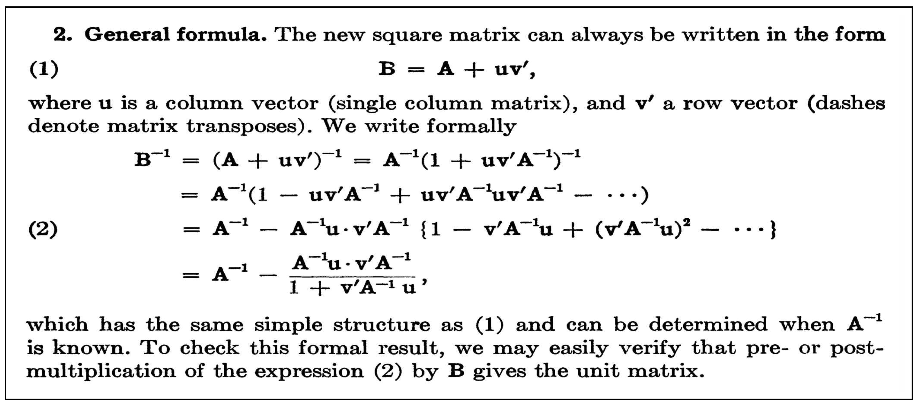
First, we begin the discussion of direct derivations with the approach Bartlett used in [37] to derive Formula (2). To preserve related historical contents faithfully, we use a screenshot. As shown in Figure 1, Bartlett’s derivation indeed looks succinct and beautiful.

However, Bartlett’s derivation is incomplete: First, the expansion of ${(I+u{v}^{\prime }{A}^{-1})}^{-1}$ into the Neumann series needs the condition $\rho (u{v}^{\prime }{A}^{-1})<1$, where $\rho ()$ denotes the spectral radius. Since $u{v}^{\prime }{A}^{-1}$ is rank-1, this condition reduces to $|v^{\prime }{A}^{-1}u|<1$. Second, the final step summing up the binomial series also requires $|v^{\prime }{A}^{-1}u|<1$. However, the inverse Formula (2) can hold for any u and v whenever $v^{\prime }{A}^{-1}u\ne -1$. Therefore, Bartlett’s derivation missed the larger region $|v^{\prime }{A}^{-1}u|>1$. However, Bartlett was careful to mention that the derived formula can be further verified by checking $B^{-1}B=I$ or $B{B}^{-1}=I$.

Bartlett’s derivation can be fixed by a suitable scaling, but it involves more than what is shown in Figure 1. The derivation—published by a pioneer and expert in the field—signals that a complete and elementary derivation of the AHD formula is more involved than one would normally expect. This likely explains why most textbooks and tutorials adopt the approach of verification from a given inverse instead of deriving the inverse directly.

In the next two subsections we focus on direct elementary derivations from scratch. That is, we do not assume or use any information about the form of the inverse before it is derived.

From here onward, we use I to denote the identity matrix of size-n; when the size of the identity matrix differs from n, we specify it explicitly using a subindex, such as $I_k$ for the size-k identity matrix.

3.1. Elementary Direct Derivations of the Family of AHD Formulas

We directly work in the complex setting, let U and $V\in {\mathbb{C}}^{n\times k},n>k\ge 1$, and let $I-U{V}^H$ be invertible. We start by deriving the formula for ${(I-U{V}^H)}^{-1}$, which is essential for all the formulas in the AHD family. The other AHD family members follow suit easily once ${(I-U{V}^H)}^{-1}$ is derived.

We first assume that V contains orthonormal columns, $V^{H}V=I_k$. (Orthonormality is a critical stepping stone in this derivation. Our method also works if we start by assuming U to have orthonormal columns. This “symmetry” in treating both U and V will be useful when we study the conditioning bounds in Section 4.) This assumption appears to severely limit generality; however, we can readily recover the lost generality by a QR trick once we derive the simplest formula.

Since $V^{H}V=I_k$, we can extend V into a size-n unitary matrixes as $[V,V_{\perp }]$. Then,

$$\begin{array}{c}\hfill I-U{V}^H=I-[U,0]\left[\begin{array}{c}{V}^H\\ V_{\perp }^H\end{array}\right]=[V,V_{\perp }]\left(I-\left[\begin{array}{c}{V}^H\\ V_{\perp }^H\end{array}\right][U,0]\right)\left[\begin{array}{c}{V}^H\\ V_{\perp }^H\end{array}\right]\\ \hfill =[V,V_{\perp }]\left[\begin{array}{cc}{I}_k-V^{H}U& 0\\ -V_{\perp }^{H}U& I_{n-k}\end{array}\right]\left[\begin{array}{c}{V}^H\\ V_{\perp }^H\end{array}\right].\end{array}$$

(5)

This instantly makes it clear that $I-U{V}^H$ being invertible is sufficient to guarantee $I_k-V^{H}U$ to be invertible, and finding ${(I-U{V}^H)}^{-1}$ is essentially finding the inverse of the block lower triangular matrix in the middle of (5). So, the task becomes easier since finding the inverse of a $2\times 2$ block lower triangular matrix is standard via a block Gauss elimination. We only need to find the block X such that

$$\begin{array}{c}\hfill \left[\begin{array}{cc}{(I_k-V^{H}U)}^{-1}& 0\\ X& I_{n-k}\end{array}\right]\left[\begin{array}{cc}{I}_k-V^{H}U& 0\\ -V_{\perp }^{H}U& I_{n-k}\end{array}\right]=\left[\begin{array}{cc}{I}_k& \\ & I_{n-k}\end{array}\right].\end{array}$$

(6)

Equating the $(2,1)$ block on both sides gives $X=V_{\perp }^{H}U{(I_k-V^{H}U)}^{-1}$. This leads to

$$\begin{array}{c}\hfill {(I-U{V}^H)}^{-1}=[V,V_{\perp }]\left[\begin{array}{cc}{(I_k-V^{H}U)}^{-1}& 0\\ V_{\perp }^{H}U{(I_k-V^{H}U)}^{-1}& I_{n-k}\end{array}\right]\left[\begin{array}{c}{V}^H\\ V_{\perp }^H\end{array}\right]\\ \hfill =V{(I_k-V^{H}U)}^{-1}{V}^H+V_{\perp }{V}_{\perp }^{H}U{(I_k-V^{H}U)}^{-1}{V}^H+V_{\perp }{V}_{\perp }^H.\end{array}$$

(7)

To find a succinct formula for ${(I-U{V}^H)}^{-1}$, we only need some patience to simplify terms: since $V{V}^H+V_{\perp }{V}_{\perp }^H=I$, we substitute $V_{\perp }{V}_{\perp }^H$ by $I-V{V}^H$. With some reordering, equality (7) becomes

$$\begin{array}{ccc}\hfill {(I-U{V}^H)}^{-1}& =& I+U{(I_k-V^{H}U)}^{-1}{V}^H+\hfill \\ & & V{(I_k-V^{H}U)}^{-1}{V}^H-V{V}^H-V{V}^{H}U{(I_k-V^{H}U)}^{-1}{V}^H.\hfill \end{array}$$

(8)

The last three terms cancel out because

$$\begin{array}{c}\hfill V{(I_k-V^{H}U)}^{-1}{V}^H-V{V}^H=V({(I_k-V^{H}U)}^{-1}-I_k)V^H\\ \hfill =V(I_k-(I_k-V^{H}U)){(I_k-V^{H}U)}^{-1}{V}^H=V{V}^{H}U{(I_k-V^{H}U)}^{-1}{V}^H.\end{array}$$

This leads to the formula

$$\begin{array}{c}\hfill {(I-U{V}^H)}^{-1}=I+U{(I_k-V^{H}U)}^{-1}{V}^H.\end{array}$$

(9)

The above derivation of (9) appears lengthy with all details written down, but it is rather straightforward. However, the straightforwardness is obtained by assuming V to have orthonormal columns, allowing V to be augmented into a unitary matrix $[V,V_{\perp }]$. After which the orthonormality quickly reveals the essential structure of the sought inverse. Once derived, it becomes easy to check via multiplication that (9) is the inverse without needing the condition $V^{H}V=I_k$. However, we need neither “verification” nor the condition $V^{H}V=I_k$.

For the general case where V may not have orthonormal columns, we can apply QR factorization to V. Let $V=QR$, where $Q^{H}Q=I_k$, and R is triangular (not necessarily invertible); then, we combine the $R^H$ factor with U, leading to $I-U{V}^H=I-(U{R}^H)Q^H$, for which Formula (9) can be readily applied:

$$\begin{array}{ccc}\hfill {(I-U{V}^H)}^{-1}& =& {(I-U{R}^H{Q}^H)}^{-1}\hfill \end{array}$$

$$\begin{array}{ccc}& =& I+U{R}^H{(I_k-Q^{H}U{R}^H)}^{-1}{Q}^H\hfill \end{array}$$

(10)

$$\begin{array}{ccc}& =& I+U{(I_k-R^H{Q}^{H}U)}^{-1}{R}^H{Q}^H\hfill \\ & =& I+U{(I_k-V^{H}U)}^{-1}{V}^H.\hfill \end{array}$$

(11)

The terms (10) and (11) are equal because

$$R^H{(I_k-Q^{H}U{R}^H)}^{-1}={(I_k-R^H{Q}^{H}U)}^{-1}{R}^H⟺(I_k-R^H{Q}^{H}U)R^H=R^H(I_k-Q^{H}U{R}^H).$$

(12)

The right part in (12) is obvious. The left part in (12) is sometimes called the push-through identity.

Therefore, Formula (9) holds for general U and V under the basic condition that $I-V^{H}U$ is invertible. We derive (9) from scratch, using no previous knowledge about ${(I-U{V}^H)}^{-1}$.

Now, we address the other members in the AHD family. First, the I in (9) needs to be replaced by an invertible $A\in {\mathbb{C}}^{n\times n}$. We only need the basic condition that $A-U{V}^H$ is invertible. Then, by Formula (9), we obtain

$$\begin{array}{ccc}\hfill {(A-U{V}^H)}^{-1}& =& {(A(I-A^{-1}U{V}^H))}^{-1}={(I-A^{-1}U{V}^H)}^{-1}{A}^{-1}\hfill \\ & =& (I+A^{-1}U{(I_k-V^H{A}^{-1}U)}^{-1}{V}^H)A^{-1}\hfill \\ & =& A^{-1}+A^{-1}U{(I_k-V^H{A}^{-1}U)}^{-1}{V}^H{A}^{-1}.\hfill \end{array}$$

(13)

Next comes the more general $UC{V}^H$ replacing $U{V}^H$, where $C\in {\mathbb{C}}^{k\times k}$. Under the basic condition that $A-UC{V}^H$ is invertible, we can easily obtain ${(A-UC{V}^H)}^{-1}$ via (13). If we group C with U and then apply (13), we obtain

$$\begin{array}{ccc}\hfill {(A-UC{V}^H)}^{-1}& =& A^{-1}+A^{-1}UC{(I_k-V^H{A}^{-1}UC)}^{-1}{V}^H{A}^{-1}.\hfill \end{array}$$

(14)

If we group C with $V^H$ and then apply (13), we obtain

$$\begin{array}{ccc}\hfill {(A-UC{V}^H)}^{-1}& =& A^{-1}+A^{-1}U{(I_k-C{V}^H{A}^{-1}U)}^{-1}C{V}^H{A}^{-1}.\hfill \end{array}$$

(15)

If C is assumed to be invertible, then from either (14) or (15) we can derive

$$\begin{array}{ccc}\hfill {(A-UC{V}^H)}^{-1}& =& A^{-1}+A^{-1}U{(C^{-1}-V^H{A}^{-1}U)}^{-1}{V}^H{A}^{-1}.\hfill \end{array}$$

(16)

Identity (16) is exactly the AHD Formula (4) that was the center of discussion in Section 2.

It is noteworthy that both (14) and (15) hold without requiring C to be invertible. In fact, Formula (15) is identical to the general formula that Henderson and Searle labeled as identity (1) to start their excellent review [7].

Also worth noting is that Woodbury in [5] appeared to seek a more general formula than (4) for the more general case where S may be singular. However, the one he obtained in [5] is (3), which is equivalent to (4) since the S in (3) must be invertible. In comparison, our elementary method derives from scratch two formulas, (14) and (15), that are more general than (4), and the process is effortless after the essential (9) is established.

There are no doubt quicker ways to derive (9). We present one method that is both simple and fast. It is even faster than the quickest derivation listed in Wikipedia (https://en.wikipedia.org/wiki/Woodbury_matrix_identity, accessed in September 2025), since it does not need to use the push-through identity.

Denote $X={(I-U{V}^H)}^{-1}$, then

$$\begin{array}{c}\hfill I=X(I-U{V}^H)=X-XU{V}^H.\end{array}$$

(17)

Right multiplying (17) by U leads to

$$U=XU-XU{V}^{H}U=XU(I_k-V^{H}U).$$

Moreover, since $V^{H}U$ and $U{V}^H$ have same nonzero eigenvalues, $I-U{V}^H$ being invertible guarantees $I_k-V^{H}U$ to be invertible. (The fastest derivation in Wikipedia missed a step to show that ${(I_k-V^{H}U)}^{-1}$ exists before using it.) Therefore,

$$\begin{array}{c}\hfill XU=U{(I_k-V^{H}U)}^{-1}.\end{array}$$

(18)

Plugging $XU$ from (18) in (17), we obtain

$$\begin{array}{c}\hfill X=I+XU{V}^H=I+U{(I_k-V^{H}U)}^{-1}{V}^H.\end{array}$$

(19)

Formula (19) is the same as (9) since $X={(I-U{V}^H)}^{-1}$.

Our method is systematic in that it can be applied directly to derive all the formulas in the AHD family.

We apply it to the more complicated ${(A-UC{V}^H)}^{-1}$ directly: Denote $X={(A-UC{V}^H)}^{-1}$, then $I=X(A-UC{V}^H)=XA-XUC{V}^H$. Right multiplying by $A^{-1}$ leads to

$$\begin{array}{c}\hfill A^{-1}=X-XUC{V}^H{A}^{-1}.\end{array}$$

(20)

Right multiplying (20) by U leads to $A^{-1}U=XU-XUC{V}^H{A}^{-1}U=XU(I_k-C{V}^H{A}^{-1}U)$. Moreover, $A-UC{V}^H$ being invertible can guarantee $I_k-C{V}^H{A}^{-1}U$ to be invertible. Therefore,

$$\begin{array}{c}\hfill XU=A^{-1}U{(I_k-C{V}^H{A}^{-1}U)}^{-1}.\end{array}$$

(21)

Plugging $XU$ from (21) in (20), we obtain

$$\begin{array}{c}\hfill X=A^{-1}+XUC{V}^H{A}^{-1}=A^{-1}+A^{-1}U{(I_k-C{V}^H{A}^{-1}U)}^{-1}C{V}^H{A}^{-1}.\end{array}$$

(22)

Formula (22) is the general (15) without requiring C to be invertible.

Similarly, right multiplying (20) by $UC$ leads to $A^{-1}UC=XUC(I_k-V^H{A}^{-1}UC)$. The assumption of $A-UC{V}^H$ being invertible guarantees $I_k-V^H{A}^{-1}UC$ to be invertible. Therefore,

$$\begin{array}{c}\hfill XUC=A^{-1}UC{(I_k-V^H{A}^{-1}UC)}^{-1}.\end{array}$$

(23)

Plugging $XUC$ from (23) in (20), we obtain

$$\begin{array}{c}\hfill X=A^{-1}+XUC{V}^H{A}^{-1}=A^{-1}+A^{-1}UC{(I_k-V^H{A}^{-1}UC)}^{-1}{V}^H{A}^{-1}.\end{array}$$

(24)

Formula (24) is the general (14) without requiring C to be invertible.

If C is further assumed to be invertible, we obtain the same (16) from either (22) or (24) in just one more step by pulling C into the inverse of the smaller $k\times k$ matrix.

Our little method is so fast that it makes the common practice of proving the formulas through verification appear slow and burdensome. Recall that the common practice is to prove that an explicitly given inverse formula is true by verifying that its product with the original matrix is the identity matrix.

The given complicated inverse formula may occasionally contain typos, which can make the lengthy verification via matrix multiplications even more taxing. In contrast, our method can quickly derive the inverse formulas from scratch, making it unnecessary to depend on a given inverse. Our method is also more systematic for the derivation than all the other methods we are aware of in the existing literature.

Even though our first method described earlier appears much slower and lengthier than the fast method just presented, it is more elementary: It does not need to resort to eigenvalues or determinant identities such as

$$det(A-UC{V}^H)=det(A)det(I_k-C{V}^H{A}^{-1}U)=det(A)det(I_k-V^H{A}^{-1}UC),$$

to establish the invertibility of the two size $k\times k$ matrices needed at (21) and (23). More importantly, this method is based on the idea of making U or V to have orthonormal columns, which plays a key role for improving the conditioning bounds in Section 4.

3.2. Classic Direct Derivations

In this subsection, we give an overview of the classic methods used by the pioneers to derive the formulas. What Aitken, Hotelling [32], Duncan [1], and also Guttman [2] used is an augmentation technique, which finds the inverse of a $2\times 2$ augmented matrix. Guttman in [2] coined a vivid term the enlargement principle for such a technique. The found inverse formulas may be traced back to Banachiewicz [35,36] (as cited in [7]).

The classic approaches commonly involve matrix factors containing Schur complements, although the term Schur complement has to wait a few more years to be coined by Haynsworth in 1968 [47]. Each such found AHD formula is essentially the inverse of a Schur complement [6].

During the early development, the derivations were rather complicated. For example, Hotelling [32] used four inversions of half-sized matrices for his derivation, and Waugh [33] improved Hotelling’s method by reducing four block-wise inversions into just two inversions.

A relatively recent presentation of the classic derivations includes Hager [6] and Bjorck (p. 128, [8]). We skip the details of the classic approaches, which can be found in the listed references, but we note that the classic methods are quite involved and often need several steps of derivation.

In the following, we present the details of a modified classic method that provides some simplification over the classic methods. This approach is in the same vein as the classic methods; it casts finding an inverse matrix as a problem of solving an augmented linear equation.

Under the condition that $(A-UC{V}^H)$ is invertible, solving $(A-UC{V}^H)X=M$ is equivalent to finding $X={(A-UC{V}^H)}^{-1}M$ for a matrix M of n rows. Denote $Y=C{V}^{H}X$, then $AX-UY=M$.

If C is further assumed to be invertible, then

$$\begin{array}{c}\hfill \left[\begin{array}{cc}A& -U\\ V^H& -C^{-1}\end{array}\right]\left[\begin{array}{c}X\\ Y\end{array}\right]=\left[\begin{array}{c}M\\ 0\end{array}\right].\end{array}$$

(25)

We can apply a block Gauss elimination to obtain

$$\begin{array}{c}\hfill \left[\begin{array}{cc}I& \\ -V^H{A}^{-1}& I\end{array}\right]\left[\begin{array}{cc}A& -U\\ V^H& -C^{-1}\end{array}\right]\left[\begin{array}{c}X\\ Y\end{array}\right]=\left[\begin{array}{cc}A& -U\\ 0& -C^{-1}+V^H{A}^{-1}U\end{array}\right]\left[\begin{array}{c}X\\ Y\end{array}\right]=\left[\begin{array}{c}M\\ -V^H{A}^{-1}M\end{array}\right].\end{array}$$

(26)

Then, solving backwardly, we obtain

$$\begin{array}{c}\hfill Y={(C^{-1}-V^H{A}^{-1}U)}^{-1}{V}^H{A}^{-1}M,\\ \hfill AX=M+UY=(I+U{(C^{-1}-V^H{A}^{-1}U)}^{-1}{V}^H{A}^{-1})M,\end{array}$$

(27)

$$\begin{array}{c}\hfill X=A^{-1}(I+U{(C^{-1}-V^H{A}^{-1}U)}^{-1}{V}^H{A}^{-1})M.\end{array}$$

(28)

Comparing (28) with $X={(A-UC{V}^H)}^{-1}M$, we establish

$$\begin{array}{c}\hfill {(A-UC{V}^H)}^{-1}=A^{-1}(I+U{(C^{-1}-V^H{A}^{-1}U)}^{-1}{V}^H{A}^{-1})\end{array}$$

(29)

by letting $M=I$. (Here, M can be chosen as any invertible matrix, or it can simply be a vector that loops through all columns of an invertible matrix. Both are sufficient to show that all corresponding columns on both sides of (29) are equal.)

Formula (29) is the same as (16), obtained by the simplified classic method in only a few steps.

This method is described in (pp. 82–83, [48]), although [48] does not specify its origin.

The method appears able to derive the AHD Formula (16) quickly, without any tedious calculations, and it essentially uses only one block inversion.

A careful look over this method can reveal that its origin is indeed in the classic methods used by Duncan et al. In fact, the augmented matrix in (25) is almost identical to the one used in Hager [6] (they differ only in minor notations). Two reasons make this method appear to be much quicker for the derivation than the classic methods.

First, it focuses on finding only ${(A-UC{V}^H)}^{-1}$, while the classic methods (as described in Hager [6] and Bjorck in (p. 128, [8])) have the broader goal of finding the inverse of the whole block augmented matrix, thus incurring the need for two block inverses and some more involved calculations.

Second, step (27) requires $C^{-1}-V^H{A}^{-1}U$ to be invertible, but this is not obvious under the common condition that $A-UC{V}^H$ is invertible. One would need a more involved argument using Schur complements: The $A-UC{V}^H$ is the Schur complement of $-C^{-1}$ in the augmented matrix in (25); this Schur complement being invertible guarantees the $2\times 2$ block augmented matrix in (25) to be invertible, which ensures $C^{-1}-V^H{A}^{-1}U$ to be invertible, based on (26). So, the quick derivation via this simplified method hides quite some involved steps in the background.

Even comparing with this simplified classic method that targets at deriving only ${(A-UC{V}^H)}^{-1}$ and appears fast, our two methods are still competitive: (i) they also need only one block inverse; (ii) they are straightforward and need no ingenious augmentation of matrices; (iii) they do not need the C to be invertible and can naturally derive the more general formulas (such as (14) and (15)). More importantly, our lengthier method initially reduces the V matrix into having orthonormal columns via a QR factorization and then groups the R factor with other terms. The same procedure can be applied to the U matrix. This QR trick is useful in [49] for extending the Householder reflector to reflect block matrices when a symmetry condition is lost; it is also useful for establishing the significantly improved conditioning bounds, which we discuss in the next section.

4. Effective Conditioning of the AHD Formula

A major reference on the numerical stability of the AHD formulas is Yip [30]. In [30], Yip focuses on the stability issue of computing $A^{-1}$ via (30)

$$A^{-1}=B^{-1}+B^{-1}U{(I_p-V^T{B}^{-1}U)}^{-1}{V}^T{B}^{-1},$$

(30)

for $A=B-U{V}^T$, where A and B are invertible of size $n\times n$, and U and V are of size $n\times p$ with full column rank p.

The stability of Formula (30) critically depends on $\kappa (I_p-V^T{B}^{-1}U)$, where $\kappa ()$ denotes the condition number in 2-norm. In this section, we solely use $\parallel ·\parallel$ to denote the 2-norm; thus, $\kappa (M)=\parallel M\parallel \parallel M^{-1}\parallel$ for any invertible matrix M. We also use the same notations to agree with those in [30]; thus, the AHD formula is applied to $A=B-U{V}^T$ instead of $B=A-U{V}^T$. However, the bounds obtained work for both $B=A\pm U{V}^T$.

A key result in Yip [30] is Lemma 1 listed below; this lemma establishes an upper bound for $\kappa (I_p-V^T{B}^{-1}U)$. The two theorems in [30] heavily depend on this lemma. The theoretical bounds in [30] are important in that they address the critical term in the AHD formula that is most responsible for its numerical stability. Yip [30] has been a main reference on the numerical stability of the AHD formulas (cited in, e.g., [6,18,19,20,21,22,23,26]).

Lemma 1

([30]). If A and B are nonsingular $n\times n$ matrices, and U and V are $n\times p$ matrices such that $A=B-U{V}^T$, with U and V of full column rank, then

$$\kappa (I_p-V^T{B}^{-1}U)\le min\{k_1,k_2\}\kappa (A)\kappa (B),$$

(31)

where

$$k_1={\left(\parallel U\parallel \parallel U^{+}\parallel \right)}^2,k_2={\left(\parallel V\parallel \parallel {(V^T)}^{+}\parallel \right)}^2$$

with

$$U^{+}={(U^{T}U)}^{-1}{U}^T,{(V^T)}^{+}=V{(V^{T}V)}^{-1}.$$

The proof given in [30] first derives that

$$I_p-V^T{B}^{-1}U=U^{+}A{B}^{-1}U.$$

(32)

After (32), Yip immediately follows with

$${(I_p-V^T{B}^{-1}U)}^{-1}=U^{+}B{A}^{-1}U.$$

(33)

Then, Yip obtains one branch of the bound via the following

$$\begin{array}{cc}\hfill \kappa (I_p-V^T{B}^{-1}U)& =\parallel (I_p-V^T{B}^{-1}U)\parallel \parallel {(I_p-V^T{B}^{-1}U)}^{-1}\parallel \hfill \\ \hfill & \le \parallel U^{+}A{B}^{-1}U\parallel \parallel U^{+}B{A}^{-1}U\parallel \hfill \\ \hfill & \le (\parallel U^{+}{\parallel \parallel U\parallel )}^2\parallel A\parallel \parallel B^{-1}\parallel \parallel B\parallel \parallel A^{-1}\parallel =k_1\kappa (B)\kappa (A).\hfill \end{array}$$

Finally, Yip states that the other branch of the bound $\kappa (I_p-V^T{B}^{-1}U)\le k_2\kappa (B)\kappa (A)$ can be established similarly, thus proving (31).

However, there is a gap from (32) to (33). Recall that the “reverse order law” such as ${(EF)}^{+}=F^{+}{E}^{+}$ in general does not hold when the matrices E and F are singular [50,51]; therefore, we cannot obtain (33) via ${(U^{+}XU)}^{-1}={(U^{+}XU)}^{+}=U^{+}{X}^{+}U$ since the last step may not hold. Indeed, ${(U^{+}XU)}^{-1}$ and $U^{+}{X}^{-1}U$ can differ even when both X and $U^{+}XU$ are invertible. A simple example showing that ${(U^{+}XU)}^{-1}\ne U^{+}{X}^{-1}U$ is $U=\left[\begin{array}{c}1\\ 1\end{array}\right], X=\left[\begin{array}{cc}1& 0\\ 0& 2\end{array}\right].$ Then, we have

$$\begin{array}{c}\hfill U^{+}=\frac{1}{2}\left[\begin{array}{c}1,1\end{array}\right],U^{+}XU=\frac{1}{2}[11]\left[\begin{array}{c}1\\ 2\end{array}\right]={\displaystyle \frac{3}{2}},U^{+}{X}^{-1}U=\frac{1}{2}[11]\left[\begin{array}{c}1\\ \frac{1}{2}\end{array}\right]={\displaystyle \frac{3}{4}}.\end{array}$$

So even with an invertible $X=A{B}^{-1}$, the (33) may still fail. Fortunately for (33), the U is not independent to the matrix $B{A}^{-1}$ but linked via $A=B-U{V}^T$. This condition is critical for (33) to hold. The proof needs a few steps of algebra and is given in Appendix A as Lemma A1.

Here, we provide a different proof to establish the bound (31). Our proof does not really need (33), but we need to guarantee that $I_p-V^T{B}^{-1}U$ is invertible. Although it can be done without (33), we opt to prove (33) in Lemma A1, filling a gap in [30] and at the same time showing that $I_p-V^T{B}^{-1}U$ is invertible, based on (32). The main advantage of our proof is in revealing much sharper bounds of $\kappa (I_p-V^H{B}^{-1}U)$ than (31).

Proof. 

We prove Lemma 1 in the general complex setting, where A and $B\in {\mathbb{C}}^{n\times n}$ are nonsingular, $A=B-U{V}^H$, and U and $V\in {\mathbb{C}}^{n\times p}$ have rank p. Let the QR factorization of U be $U=QR$. Since U has full column rank, we have $Q\in {\mathbb{C}}^{n\times p}$ with $Q^{H}Q=I_p$, and $R\in {\mathbb{C}}^{p\times p}$ is invertible. Therefore,

$$U^{+}={(U^{H}U)}^{-1}{U}^H=R^{-1}{Q}^H\mathrm{and}{U}^{+}U=I_p.$$

Since $A=B-U{V}^H$, we have $A{B}^{-1}U=(B-U{V}^H)B^{-1}U=U(I-V^H{B}^{-1}U)$. Left multiplying by $U^{+}$ leads to

$$I-V^H{B}^{-1}U=U^{+}A{B}^{-1}U.$$

After substituting $U=QR$ and $U^{+}=R^{-1}{Q}^H$, we obtain

$$I-V^H{B}^{-1}U=R^{-1}\left(Q^{H}A{B}^{-1}Q\right)R.$$

Let $S=Q^{H}A{B}^{-1}Q$, then

$$\begin{array}{c}\hfill I-V^H{B}^{-1}U=R^{-1}SR.\end{array}$$

(34)

By the definition of the condition number and the sub-multiplicity of the 2-norm, we have

$$\begin{array}{c}\hfill \kappa (R^{-1}SR)=\parallel R^{-1}SR\parallel \parallel {(R^{-1}SR)}^{-1}\parallel \le (\parallel R\parallel \parallel R^{-1}{\parallel )}^2\kappa (S)=k_1\kappa (S).\end{array}$$

(35)

The last equality is because $\parallel R\parallel \parallel R^{-1}\parallel =\kappa (R)=\parallel U\parallel \parallel U^{+}\parallel$.

Now, we bound $\kappa (S)$ by $\kappa (A{B}^{-1})$, for which we need to compare singular values. For this, we use the variational expressions of singular values. Assume $x,y,u,v$ are nonzero vectors, then

$$\begin{array}{ccc}\hfill {\sigma }_{max}(A{B}^{-1})& =& \underset{x,y\in {\mathbb{C}}^{n\times n}}{max}{\displaystyle \frac{|x^{H}A{B}^{-1}y|}{\parallel x\parallel \parallel y\parallel }}\hfill \\ & \ge & \underset{x=Qu,y=Qv}{max}{\displaystyle \frac{|u^H{Q}^{H}A{B}^{-1}Qv|}{\parallel Qu\parallel \parallel Qv\parallel }}=\underset{u,v\in {\mathbb{C}}^{p\times p}}{max}{\displaystyle \frac{|u^{H}Sv|}{\parallel u\parallel \parallel v\parallel }}={\sigma }_{max}(S),\hfill \\ \hfill {\sigma }_{min}(A{B}^{-1})& =& \underset{x,y\in {\mathbb{C}}^{n\times n}}{min}{\displaystyle \frac{|x^{H}A{B}^{-1}y|}{\parallel x\parallel \parallel y\parallel }}\hfill \\ & \le & \underset{x=Qu,y=Qv}{min}{\displaystyle \frac{|u^H{Q}^{H}A{B}^{-1}Qv|}{\parallel Qu\parallel \parallel Qv\parallel }}=\underset{u,v\in {\mathbb{C}}^{p\times p}}{min}{\displaystyle \frac{|u^{H}Sv|}{\parallel u\parallel \parallel v\parallel }}={\sigma }_{min}(S).\hfill \end{array}$$

Therefore,

$$\begin{array}{c}\hfill \kappa (S)={\displaystyle \frac{{\sigma }_{max}(S)}{{\sigma }_{min}(S)}}\le {\displaystyle \frac{{\sigma }_{max}(A{B}^{-1})}{{\sigma }_{min}(A{B}^{-1})}}=\kappa (A{B}^{-1}).\end{array}$$

(36)

Combining bounds (35) and (36), we obtain

$$\begin{array}{c}\hfill \kappa (I-V^H{B}^{-1}U)\le k_1\kappa (A{B}^{-1}).\end{array}$$

(37)

The same argument can be used to establish the other bound involving V. We only need to apply the argument to $A^H=B^H-V{U}^H$. This involves replacing A by $A^H$, and B by $B^H$, and switching U and V in the above proof. So, we obtain

$$\kappa (I_p-U^H{B}^{-H}V)\le k_2\kappa (A^H{B}^{-H}).$$

Since $\kappa (I_p-U^H{B}^{-H}V)=\kappa (I_p-V^H{B}^{-1}U)$ and $\kappa (A^H{B}^{-H})=\kappa (B^{-1}A)$, we obtain

$$\begin{array}{c}\hfill \kappa (I_p-V^H{B}^{-1}U)\le k_2\kappa (B^{-1}A).\end{array}$$

(38)

Combining the two bounds (37) and (38), we obtain

$$\begin{array}{c}\hfill \kappa (I_p-V^H{B}^{-1}U)\le min\{k_1\kappa (A{B}^{-1}),k_2\kappa (B^{-1}A)\}.\end{array}$$

(39)

Finally, since $max\{\kappa (A{B}^{-1}),\kappa (B^{-1}A)\}\le \kappa (A)\kappa (B)$, we obtain Yip’s bound (31) (in the complex setting)

$$\kappa (I_p-V^H{B}^{-1}U)\le min\{k_1,k_2\}\kappa (A)\kappa (B).$$

   □

Our proof establishes two bounds sharper than Yip’s (31). One of them is the bound (39); however, the improvement in general is moderate.

Our other bound is significantly sharper than both (39) and (31), especially when p is relatively small comparing to n, which corresponds to the more common low-rank modifications encountered in diverse applications where the AHD formulas are utilized.

Observe that (35) is

$$\begin{array}{c}\hfill \kappa (I_p-V^H{B}^{-1}U)\le k_1\kappa (Q^{H}A{B}^{-1}Q).\end{array}$$

(40)

Applying the same argument that leads to (35) to $A^H=B^H-V{U}^H$, using QR factorization of $V=\widehat{Q}\widehat{R}$, we can obtain

$$\begin{array}{c}\hfill \kappa (I_p-U^H{B}^{-H}V)\le k_2\kappa ({\widehat{Q}}^H{A}^H{B}^{-H}\widehat{Q})=k_2\kappa ({\widehat{Q}}^H{B}^{-1}A\widehat{Q}).\end{array}$$

(41)

We can also obtain (41) without using the transpose trick as done above. Since ${(V^H)}^{+}=V{(V^{H}V)}^{-1}$, we have $V^H{(V^H)}^{+}=I_p$. Left multiplying $A=B-U{V}^H$ by $V^H{B}^{-1}$ leads to $V^H{B}^{-1}A=V^H-V^H{B}^{-1}U{V}^H$; further, right multiplying by ${(V^H)}^{+}$, we obtain

$$\begin{array}{c}\hfill I_p-V^H{B}^{-1}U=V^H{B}^{-1}A{(V^H)}^{+}.\end{array}$$

(42)

Identity (42) already exists in [52] and is used for other purpose there. For our purpose here, we only need to apply the QR factorization $V=\widehat{Q}\widehat{R}$ directly to (42) and then apply the same reasoning as done for the U branch. This can directly lead to the bound $\kappa (I_p-V^H{B}^{-1}U)\le k_2\kappa ({\widehat{Q}}^H{B}^{-1}A\widehat{Q})$, which is the same as (41) but without using the quicker transpose trick.

Combining (40) and (41), we obtain a tighter bound, which we summarize as bound (43) in Lemma 2.

Lemma 2.

Assume $A=B-U{V}^H$, where A and $B\in {\mathbb{C}}^{n\times n}$ are nonsingular, and U and $V\in {\mathbb{C}}^{n\times p}$ have rank p. Let $k_1={\left(\parallel U\parallel \parallel U^{+}\parallel \right)}^2$ and $k_2={\left(\parallel V\parallel \parallel V^{+}\parallel \right)}^2$, where ${()}^{+}$ denotes the Moore–Penrose pseudo-inverse. Let the QR factorizations of U and V be, respectively, $U=QR$ and $V=\widehat{Q}\widehat{R}$, then

$$\begin{array}{ccc}\hfill \kappa (I_p-V^H{B}^{-1}U)& \le & min\{k_1\kappa (Q^{H}A{B}^{-1}Q),k_2\kappa ({\widehat{Q}}^H{B}^{-1}A\widehat{Q})\}\hfill \end{array}$$

(43)

$$\begin{array}{ccc}& \le & min\{k_1\kappa (A{B}^{-1}),k_2\kappa (B^{-1}A)\}\hfill \end{array}$$

(44)

$$\begin{array}{ccc}& \le & min\{k_1,k_2\}\kappa (A)\kappa (B).\hfill \end{array}$$

(45)

We call (43) the compressed bound since it involves compressing the matrices $A{B}^{-1}$ and $B^{-1}A$ on the range subspaces generated by U and V, respectively. The sharper compressed bound may be considered as the effective conditioning for $\kappa (I_p-V^H{B}^{-1}U)$. This is because bound (43) shows that the components of the matrices $A{B}^{-1}$ and $B^{-1}A$ outside the compressed parts are ineffective in affecting $\kappa (I_p-V^H{B}^{-1}U)$. Including only the effective components significantly improves the quality of the bounds.

Bound (44) is denoted by the mod bound (meaning the modified Yip’s bound), and we call (45) the Yip’s bound, which is the same as (31) but allows all $A,B,U,V$ to be complex.

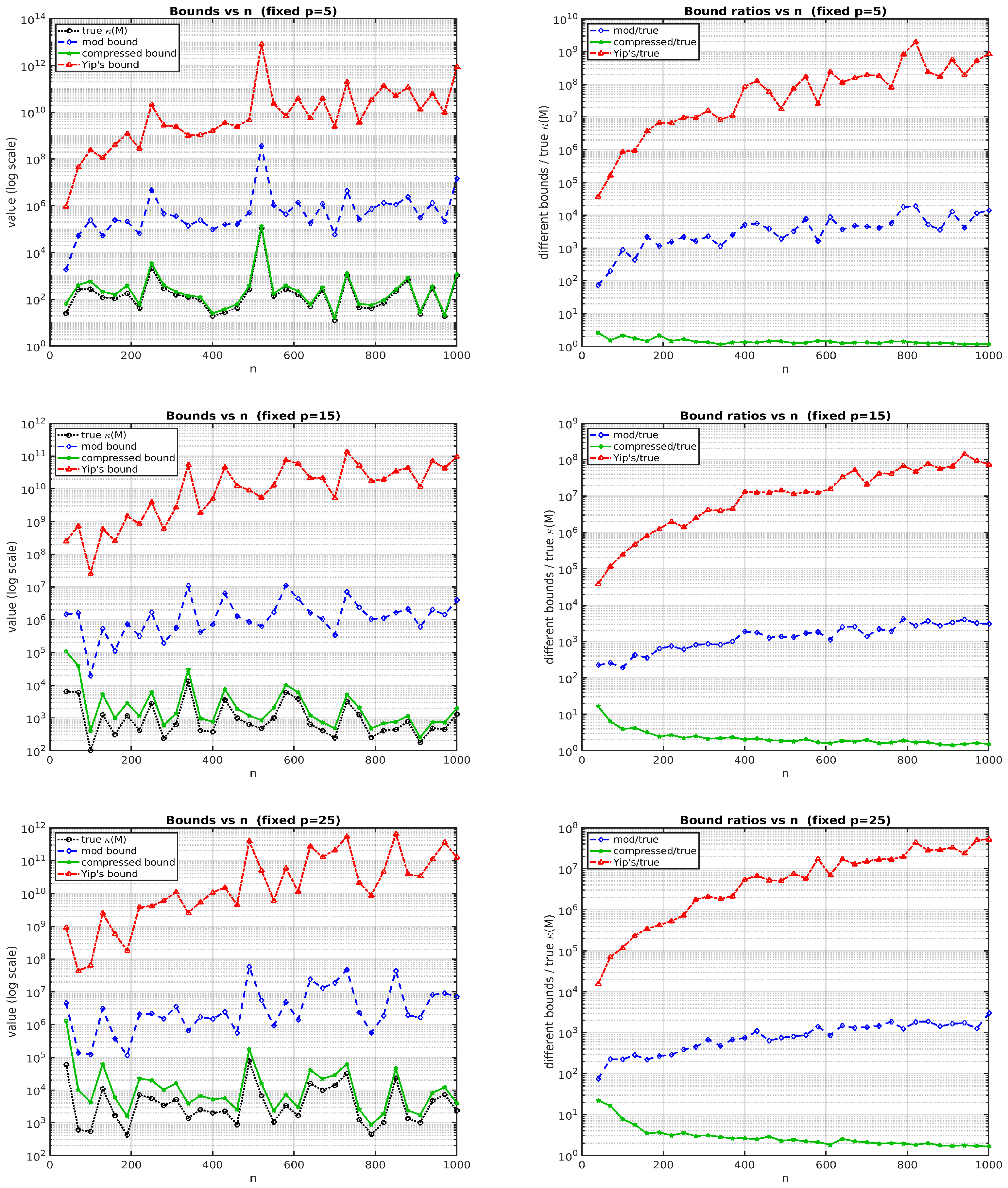
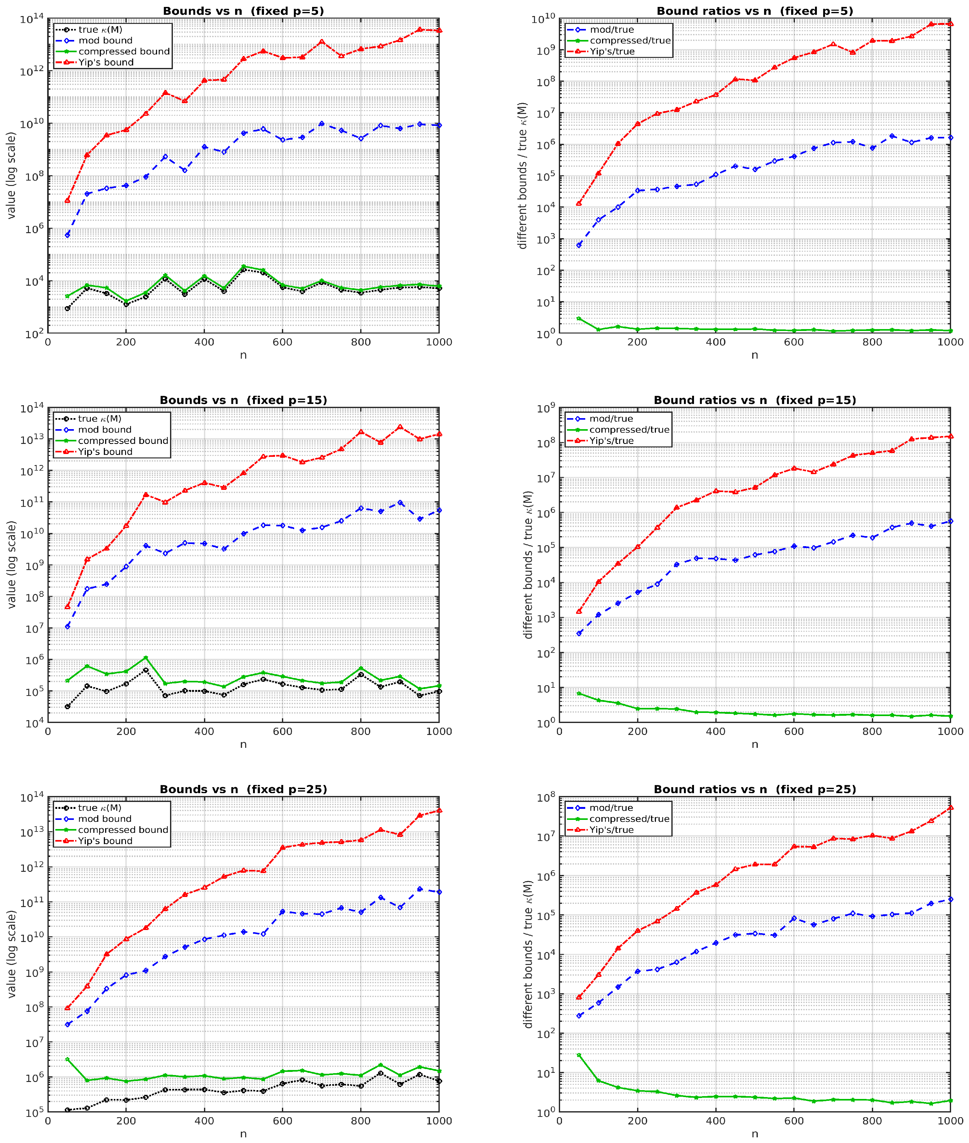
For the random matrix generations in the numerical experiments presented in Figure 2 and Figure 3, there is no essential difference in using the uniform distribution rand() or the standard normal distribution randn(). The Matlab code used for numerical tests is available at the url provided in the Data Availability Statement at the end of this paper.

As seen from Figure 2 and Figure 3, the compressed bound (43) in general can capture the true value of $\kappa (I_p-V^H{B}^{-1}U)$ remarkably well, while the other two bounds (44) and (45) tend to significantly overestimate the true condition number.

In [30], Yip mentioned that his bound (31) can become overly pessimistic. We may apply bound (43) for a feasible explanation: The effective (or active) components affecting $\kappa (I_p-V^H{B}^{-1}U)$ are in the compressed $p\times p$ matrices $Q^{H}A{B}^{-1}Q$ and ${\widehat{Q}}^H{B}^{-1}A\widehat{Q}$, while the larger uncompressed $n\times n$ matrices $A{B}^{-1}$ and $B^{-1}A$ contain mostly ineffective components for measuring $\kappa (I_p-V^H{B}^{-1}U)$ since theoretically bound (43) does not need these components. Keeping the ineffective components in the bounds only contributes to making the bounds overestimate the true $\kappa (I_p-V^H{B}^{-1}U)$. Separating the matrices as done in (31) and (45) may cause even larger overestimates leading to more pessimistic bounds.

Our bound (43) reveals that the true $\kappa (I_p-V^H{B}^{-1}U)$ mainly depends on the conditioning of the compressed matrices $Q^{H}A{B}^{-1}Q$ and ${\widehat{Q}}^H{B}^{-1}A\widehat{Q}$, which can be much smaller than the conditioning of the uncompressed $A{B}^{-1}$ or $B^{-1}A$. The low-rank perturbation or low-rank update commonly encountered in diverse applications implies that $p\ll n$, for which the two $p\times p$ compressed matrices can naturally have a much smaller condition number than the two $n\times n$ uncompressed matrices.

Voet et al. (p. 124, [19]) and Zhang et al. (p. 1591, [18]) both mentioned that although stability concerns about the AHD formulas have been raised by Yip [30], their algorithms applying the formulas encounter no numerical instabilities. The fact that the family of AHD formulas has continued to shine in diverse fields implies that numerical stability, especially in the low rank $p\ll n$ case, is far better than bounds in Yip [30] suggest. Our sharper bound (43) can provide theoretical support to the observations made in [18,19] and in other cases where the formulas naturally perform stably.

Since the compressed bound (43) can closely bound the true value of $\kappa (I_p-V^H{B}^{-1}U)$, which is an effective indicator of the stability when applying Formula (30) to compute $A^{-1}$, we consider (43) as an effective conditioning bound of the associated AHD formula.

Certainly numerical methods, especially those employing matrix inverses, do have numerical stability concerns. The alarm sound in [30] is based on a valid concern. However, the bound (45) from [30] can severely overestimate the ill-conditioning, making the AHD formulas appear prone to be unstable. The fact that the AHD formulas have been employed in diverse fields for satisfactory numerical performance implies that they are in general not as ill-conditioned as the bound (45) suggests. Keeping only the effective components in the bound as in (43) provides a more realistic view of the true conditioning.

We can improve bound (43) even further by the QR technique utilized in Section 3.1, which is to perform QR factorization to U or V to make at least one of them to have orthonormal columns, so that $k_1=1$ or $k_2=1$, and then combine the R-factor with the other term so that $U{V}^H$ stay unchanged. We state the bounds in Theorem 1.

Theorem 1.

If A and B are nonsingular $n\times n$ matrices, and U and V are $n\times p$ matrices such that $A=B-U{V}^H$, with U and V of full column rank. Let the QR factorizations of U and V be, respectively, $U=QR$ and $V=\widehat{Q}\widehat{R}$. Let $M_1=I_p-{(V{R}^H)}^H{B}^{-1}Q$ and $M_2=I_p-{\widehat{Q}}^H{B}^{-1}U{\widehat{R}}^H$. Then,

$$\begin{array}{ccc}\hfill min\{\kappa (M_1),\kappa (M_2)\}& \le & min\{\kappa (Q^{H}A{B}^{-1}Q),\kappa ({\widehat{Q}}^H{B}^{-1}A\widehat{Q})\}\hfill \end{array}$$

(46)

$$\begin{array}{ccc}& \le & min\{\kappa (A{B}^{-1}),\kappa (B^{-1}A)\}\hfill \end{array}$$

(47)

$$\begin{array}{ccc}& \le & \kappa (A)\kappa (B).\hfill \end{array}$$

(48)

Proof. 

Since $A=B-U{V}^H=B-QR{V}^H=B-U{(\widehat{Q}\widehat{R})}^H$, we associate R with V and $\widehat{R}$ with U and then apply Lemma 2. We have the following two cases:

$$\begin{array}{cc}\hfill M_1=I_p-{(V{R}^H)}^H{B}^{-1}Q& \mathrm{using}U{V}^H=Q{(V{R}^H)}^H,\\ \hfill M_2=I_p-{\widehat{Q}}^H{B}^{-1}(U{\widehat{R}}^H)& \mathrm{using}U{V}^H=(U{\widehat{R}}^H){\widehat{Q}}^H.\end{array}$$

For $M_1$, the corresponding $k_1$ in Lemma 2 is $k_1={\kappa }^2(Q)=1$. Similarly for $M_2$, the corresponding $k_2$ in Lemma 2 is $k_2={\kappa }^2(\widehat{Q})=1$.

Therefore, by Lemma 2, we have $\kappa (M_1)\le \kappa (Q^{H}A{B}^{-1}Q)$ and $\kappa (M_2)\le \kappa ({\widehat{Q}}^H{B}^{-1}A\widehat{Q})$. Combining them establishes (46).

The other two bounds (47) and (48) hold because the same reasoning in our proof of Lemma 1 shows they are the upper bounds in nondecreasing order of the compressed upper bound in (46). □

In Theorem 1, the $M_1$ and $M_2$ correspond to computing $A^{-1}$ via (49) and (50), respectively,

$$\begin{array}{cc}\hfill A^{-1}& =B^{-1}+B^{-1}Q{(I_p-R{V}^H{B}^{-1}Q)}^{-1}R{V}^H{B}^{-1},\hfill \end{array}$$

(49)

$$\begin{array}{cc}\hfill A^{-1}& =B^{-1}+B^{-1}U{\widehat{R}}^H{(I_p-{\widehat{Q}}^H{B}^{-1}U{\widehat{R}}^H)}^{-1}{\widehat{Q}}^H{B}^{-1}.\hfill \end{array}$$

(50)

Lemma 2 shows that an ill-conditioned U and V may worsen the conditioning of the capacitance matrix $M=I_p-V^H{B}^{-1}U$, owing to the presence of $k_1={\kappa }^2(U)$ and $k_2={\kappa }^2(V)$ in the compressed bound. In contrast, Theorem 1 shows that one can mitigate the ill effect of a large $k_1$ or $k_2$ by applying the QR trick to U or V so that the conditioning of the reordered capacitance matrix $M_1$ or $M_2$ is not negatively affected because the compressed bound (46) guarantees no influence from $k_1$ or $k_2$.

If $k_1$ or $k_2$ is moderate, one does not need to apply the QR trick, and the compressed bound in Lemma 2 already can explain the good stability observed in many applications, including those in [18,19]. However, the QR trick will be particularly beneficial when both $k_1$ and $k_2$ happen to be large. In this case, if $k_1\gg k_2$, one can apply the QR trick to the ill-conditioned U and compute $A^{-1}$ via (49); if $k_1\ll k_2$, one can apply the QR trick to the ill-conditioned V and compute $A^{-1}$ via (50). Then, bound (46) shows that $min\{\kappa (M_1),\kappa (M_2)\}$ has a good chance to stay well-bounded.

Numerical stability concerns both the way obtaining $A^{-1}$ and later applying this $A^{-1}$. If the QR trick needs to be invoked and the $A^{-1}$ is obtained via (49) or (50), one may wonder if the extra R in (49) outside the inverse of $M_1$, or the extra $\widehat{R}$ in (50) outside the inverse of $M_2$, may cause extra instability. This concern is based on $\kappa (R)=\kappa (U)$ and $\kappa (\widehat{R})=\kappa (V)$, which can be large when U and V are ill-conditioned. However, both obtaining $A^{-1}$ and later applying this $A^{-1}$ do not need the extra R or $\widehat{R}$ to be further inverted; thus, they do not post extra instability. (Recall that multiplying by a matrix with tiny singular values does not pose instability; it is multiplying by the inverse of such a matrix that poses instability.) Therefore, if the compressed bound (46) is moderate, then the stability associated with $A^{-1}$ is comparable to the stability provided by $B^{-1}$.

Bound (46) is our compressed bound obtained after applying the QR trick. Bound (48) is essentially Yip’s bound from the two Theorems in [30] based on Lemma 1. Since both (46) and (48) are not influenced by $k_1$ or $k_2$, the comparisons are similar to those observed in Figure 2 and Figure 3 based on Lemma 2, with the y-axis values divided by $k_1$ or $k_2$.

5. Conclusions

In Section 2, we examine relevant historical documents related to the Sherman–Morrison–Woodbury (SMW) formula and argue that at least an equally deserving name for the same formula is the Aitken–Hotelling–Duncan (AHD) formula.

In Section 3, we present two elementary direct derivations of the AHD formula: The slower method is more elementary, but it can clearly show the main structure and connections among progressively complicated formulas in the AHD family, and it also introduces a QR trick that is useful for developing our compressed conditioning bound. The faster method is simple and systematic for deriving all formulas in the AHD family. It frees a learner from depending on a given formula of the inverse and then proving via verification. The whole process deriving the formula using our fast method may be quicker than verifying via matrix–matrix products that a given inverse formula is indeed the inverse.

In Section 4, we develop significant improvements over the classic conditioning bounds of Yip [30]. The improvements are based on our analysis that the conditioning of the capacitance matrix effectively depends only on two size $p\times p$ compressed matrices. In contrast, Yip’s bounds use the uncompressed size $n\times n$ matrices, which keep many ineffective components in the bounds, potentially leading to severe overestimates. Numerical experiments show that our compressed bound can be several million times sharper than Yip’s bound.

Yip [30] remains a major reference on the stability of the AHD formula since its publication in 1986. It is cited by most of the later publications that are concerned about numerical stability of the formula. However, the citations are more for concerns on potential instability instead of stability. This is because the bounds in [30] often become pessimistically large, implying that instability may be common. Our tightened bounds shed a clearer light on the stability issue related to the AHD formula: The effective conditioning in general can be much smaller than Yip’s bounds suggest. This implies that overall the AHD formula can naturally have numerical stability instead of instability, especially in the low-rank update ($p\ll n$) scenarios commonly encountered in real applications for which the formula is employed. Our compressed bounds can explain why the formula has performed reliably for decades in diverse fields and continues to find successful applications in emerging fields.