Article

A Dual-Branch Spatio-Temporal Feature Differencing Method for Robust rPPG Estimation

1
AI Graduate School, Gwangju Institute of Science and Technology, Gwangju 61005, Republic of Korea
2
Department of AI, Chonnam National University, Gwangju 61186, Republic of Korea
*
Authors to whom correspondence should be addressed.
Mathematics 2025, 13(23), 3830; https://doi.org/10.3390/math13233830
Submission received: 5 November 2025 / Revised: 21 November 2025 / Accepted: 26 November 2025 / Published: 29 November 2025

Abstract

Remote photoplethysmography (rPPG) is a non-contact technology that estimates physiological signals, such as Heart Rate (HR), by capturing subtle skin color changes caused by periodic blood volume variations using only a standard RGB camera. While cost-effective and convenient, it suffers from a fundamental limitation: performance degrades severely in dynamic environments due to susceptibility to noise, such as abrupt illumination changes or motion blur. This study presents a deep learning framework that combines two structural modifications to ensure robustness in dynamic environments, specifically modeling movement noise and illumination change noise. The proposed framework structurally cancels global disturbances, such as illumination changes or global motion, through a dual-branch pipeline that encodes the face and background in parallel after Video Color Magnification (VCM) and then performs differencing. Subsequently, it utilizes a structure that injects a Temporal Shift Module (TSM) into the Spatio-Temporal Feature Extraction (SSFE) block to preserve long- and short-term temporal correlations and smooth noise, even amidst short and irregular movements. We measured MAE, RMSE, and correlation on the standard dataset UBFC-rPPG under four noise conditions: clean, illumination change noise, Movement Noise, Both Noise and the real-world in-vehicle dataset MR-NIRP (Stationary and Driving). Experimental results showed that the proposed method achieved consistent error reduction and correlation improvement compared to the VS-Net baseline in the illumination change noise-only and combined noise environments (UBFC-rPPG) and in the high-noise driving scenario (MR-NIRP). It maintained competitive performance in motion-only noise. Conversely, a modest performance disadvantage was observed under clean conditions (UBFC) and quasi-clean stationary conditions (MR-NIRP), interpreted as a design trade-off focused on global noise cancellation and temporal smoothing. Ablation studies demonstrated that the dual-branch pipeline is the primary contributor under illumination change noise, while TSM is the key contributor under movement noise, and that the combination of both elements achieves optimal robustness in the most complex scenarios.

1. Introduction

Remote photoplethysmography (rPPG) is a non-contact technology that estimates physiological signals, such as Heart Rate (HR), by capturing subtle skin color changes induced by periodic blood volume variations using only a standard RGB camera [1,2]. Its advantage of enabling measurement with only video, without wearables or electrodes, drives its significant potential for expansion into real-world applications such as medicine, healthcare, and driver monitoring [3,4]. However, rPPG signals have a low amplitude compared to the video signal and possess a fundamental limitation of being highly sensitive to environmental disturbances such as illumination changes, subject/camera motion, and compression noise [5,6]. Ultimately, achieving both the amplification and quality preservation of the weak signal, and robustness against real-world noise simultaneously, is the key challenge.
Initially, traditional video amplification methods like Eulerian Video Magnification (EVM) [7] and Phase-based Video Magnification (PVM) were dominant. These methods filter and amplify color/luminance variations in the cardiac band to emphasize signals that are difficult to perceive with the naked eye. Despite the advantages of an intuitive structure and controllability, they rely on fixed linear operations, which leads to the problem of amplifying global noise along with the interest signal as global illumination changes and global motion/motion blur increase [7,8]. Visual distortions such as ringing and blurring, and limitations in adapting to scene/skin distribution differences, are also frequently observed.
The recent trend has shifted towards spatio-temporal representation learning [9,10,11,12]. In particular, VS-Net methods [13] that combine 3D patch embedding with spatio-temporal attention (Video Swin Transformer) [14] have achieved very high accuracy under static and clean conditions by jointly modeling spatial correlations between skin regions and the temporal periodicity of heartbeats. However, in real-world dynamic environments—for example, inside vehicles with rapid illumination changes at tunnel entrances/exits, strobing from windows/trees, and global motion/motion blur from road irregularities and vehicle vibrations—performance markedly degrades. This is because numerous noises appear commonly across the entire frame, making them difficult to remove using only spatio-temporal periodicity; short, irregular impulsive noises momentarily mask the slow rPPG signal, hindering long- and short-term dependency learning; and low-frequency drift heavily disrupts the input distribution. While the performance of periodicity preservation itself remains good, robustly estimating that periodicity amidst global noise and impulsive motion remains an unsolved challenge.
We proposes a framework with a new structure to structurally bridge this gap. To counter global noise and low-frequency drift, we introduce a Foreground-Background Dual-Branch Differencing pipeline that encodes the face and surrounding background in parallel at the same time point and fuses them via differencing, inspired by prior work on two-stream processing [15]. Utilizing the fact that physiological signals do not exist in the background while noise is reflected in both the foreground and background, this method amplifies the heartbeat band variation first, then cancels the simultaneous variations from the background branch, thereby suppressing global illumination change/motion components and increasing the preservation rate of the signal of interest. To address short and irregular impulsive noise in the real world, we propose a structure that injects a Temporal Shift Module (TSM) [16] inside the Spatio-Temporal Feature Extraction (SSFE) block, allowing features to be circulated between adjacent frames without increasing parameters. This shift helps to capture long-term periodicity and short-term variations simultaneously [17], smoothing momentary impacts or motion blur to maintain the low-frequency rPPG signal. In short, we present a pipeline that reveals the signal through amplification, removes global noise through background differencing, and withstands impulsive disturbances through shift-based spatio-temporal coupling.
The proposed methodology acts as a framework that prioritizes consistency and reliability in real-world scenarios where global noise and abnormal motion coexist, without significantly compromising accuracy. We verify the robustness of the proposed method by systematically organizing single and composite disturbances on UBFC [18], representing indoor static environments, and MR-NIRP [3,4], representing actual in-vehicle environments. Consequently, this study maintains the preservation of rPPG periodicity as a central value but presents a structural alternative to ensure this periodicity does not collapse under realistic disturbances, thereby increasing the feasibility of applying rPPG to real-world sites such as driver monitoring [3] and remote biometric measurement under mixed illumination.

2. Related Works

2.1. Video Color Magnification

Video Color Magnification (VCM) is a technique that amplifies subtle periodic changes in the color or luminance of video frames to visualize and enhance physiological signals that are difficult to distinguish with the naked eye. In the context of rPPG, the faint skin color changes within the cardiac frequency band are the signal of interest, and VCM selectively boosts the varying components in this band to increase the preservation rate of the target signal.
Early traditional approaches were led by the EVM family [7]. Spatially, these methods perform multi-resolution decomposition using image pyramids, and temporally, they apply a band-pass filter to amplify only the target frequency band before synthesizing the result. This line includes not only the classic EVM [7], which directly amplifies luminance (amplitude) variations, but also PVM, which uses complex steerable pyramids to amplify local phase changes. PVM offers advantages such as relatively better preservation of edges/textures and partial mitigation of large structural distortions or ringing artifacts in the output. Nevertheless, both methods rely on fixed linear filters/phase manipulations, leading to pronounced side effects where global noise is amplified along with the signal as illumination changes or camera/subject motion increases [7]. They are particularly vulnerable to low-frequency drift caused by auto-exposure/white balance, illumination changes, and motion blur, resulting in problems like distortion, intensified blurring, and ringing in the output video. Furthermore, they struggle to adapt to variations in scene/subject distribution and fail to capture valid information outside the set filter band or non-linear interactions.
To overcome these limitations, learning-based video magnification (LVM) was proposed [8]. A neural network comprising an encoder–manipulator–decoder is trained to extract, amplify, and reconstruct the target components from the input sequence. The encoder extracts features from frame pairs, the manipulator takes the structural differences between two time points to amplify components in the target band, and the decoder reconstructs the amplified result back into the image or feature space [8]. Thanks to its data-driven nature, this approach has shown superior results compared to traditional EVM in aspects like texture preservation, mitigation of color distortion, and relative suppression of low-frequency illumination changes [8,19]. Nevertheless, LVM still has remaining limitations. Signals strongly present across the entire frame, such as global illumination changes or camera shake, are easily amplified by the network along with the signal of interest [8]. This means that even if the frequency band of the target for amplification is matched, global noise might be co-amplified, potentially leading to no improvement or even degradation in the preservation rate of the signal of interest in the rPPG signal. The generalization of the amplifier decreases when the training distribution mismatches the actual test distribution, and if the statistical differences between background and skin regions are not explicitly handled, leakage of background-originating global noise can persist [15].

2.2. VS-Net

VS-Net is a deep learning model for video-based rPPG measurement, combining LVM with a spatio-temporal transformer structure [13]. The model first amplifies subtle skin color changes in the input video using a deep neural network, then models local and global spatio-temporal interactions within the amplified frames using Video Swin Transformer blocks [14], which combine multi-head self-attention and convolution. Notably, the Video Swin Transformer effectively extracts spatio-temporal features by capturing local relationships within each window using 3D windowed self-attention and shifted-window self-attention, and exchanging global information through shifts between windows [14,20].
VS-Net introduced a contrastive learning module to enhance learning for weak rPPG signals [13]. It generates positive/negative sample couples reflecting HR changes by resampling the input video at various frequencies. A loss function is then constructed to learn the similarities and differences between these couples, enabling the model to distinguish even faint signals, a concept also explored in other self-supervised rPPG works [21,22]. In the training process, the VCM was first pre-trained on a synthetic dataset simulating facial color changes, and then the entire VS-Net was fine-tuned end-to-end based on the learned weights [13]. With this design, VS-Net exhibits very high rPPG estimation accuracy in controlled environments. On the UBFC-rPPG dataset [18], it achieved improved results compared to previous methodologies in terms of MAE, RMSE, and correlation coefficient R for HR [13]. The combination of VCM and Transformer-based learning imparted robustness to illumination and posture changes, demonstrating the feasibility of stable HR measurement in low-noise indoor environments. On the other hand, VS-Net has limitations in dynamic and noisy environments. In situations involving rapid global facial movements, complex illumination changes, motion blur, or changes in camera sensor position, noise can be amplified along with color changes, potentially reducing the accuracy of rPPG signal prediction. Indeed, on dynamic and noisy datasets like MR-NIRP [3,4], its performance has been shown to be somewhat lower. In summary, while VS-Net performs very strongly in stable laboratory-level environments, it has limitations requiring further improvement for real-world scenarios involving abrupt movements or complex illumination changes.

3. Methodology

3.1. Problem Statement

The main goal of this paper is to restore the rPPG waveform and HR from RGB facial videos captured in dynamic and noisy environments. We consider an RGB facial video V = { I t } t = 1 T . The target is a band-limited blood-volume pulse (BVP) s ϕ ( t ) with fundamental frequency in [ 0.7 , 4 ] Hz (42–240 bpm) [6]. We define two simultaneous regions of interest (ROI): a facial foreground R F and a background ring R B . Spatial averaging within each ROI yields foreground/background traces that inherit frame-wide disturbances. We assume the per-pixel intensity can be decomposed into a weak physiological component, a frame-wide global nuisance, and local motion/blur artifacts, based on established rPPG reflection models [5,6], as
I t ( x ) = α ( x ) s ϕ ( t ) + g t + m t ( x ) ,
where α ( x ) scales the physiological signal spatially, g t denotes frame-wide (global) nuisances such as illumination drift and auto-exposure/white-balance fluctuations, and m t ( x ) captures irregular local disturbances. Given V, our objective is to estimate a waveform s ^ ( t ) that is temporally aligned with s ϕ ( t ) up to an unknown affine transformation and from which HR can be robustly derived via the dominant spectral peak of PSD ( s ^ ) [2,5].

3.2. Foreground–Background Dual-Branch Differencing Pipeline

In dynamic and noisy real-world scenarios, global noise, vibrations, and motion blur are reflected simultaneously across the entire frame. In contrast, the effective rPPG signal originates only from the face. Based on this fact, our method proposes a dual-branch pipeline that embeds the face and its surrounding area from the same time point using identical encoders, and then cancels common components by differencing the amplified representations from the two branches [15]. Since the background contains almost no physiological periodic signal, the differencing aims to remove global noise and amplify only the signal of interest.
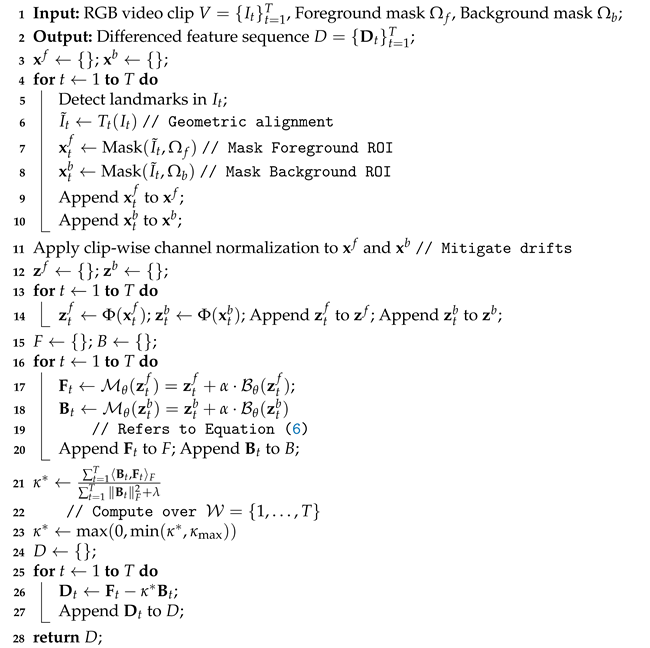
This section proposes a dual-branch differencing pipeline that structurally cancels global illumination change noise and movement noise by differencing the face representation and the background representation after VCM. The architecture of this framework is illustrated in Figure 1, and the detailed procedure is described in Algorithm 1. Given an RGB video { I t } t = 1 T , facial landmarks are detected in each frame [23], and the geometry is aligned using a similarity transformation T t to a reference template. From the aligned frame I ˜ t = T t ( I t ) , the branch inputs are constructed by masking the facial ROI Ω f and the background ROI Ω b (non-skin area):
x t f = Mask ( I ˜ t , Ω f ) R H × W × 3 , x t b = Mask ( I ˜ t , Ω b ) R H × W × 3 .
Then, clip-wise channel normalization is applied to each branch to mitigate exposure/white balance drift, and d-channel features are obtained using a shallow learnable color projection Φ ( · ) (based on 1 × 1 convolution for color mixing):
z t f = Φ ( x t f ) , z t b = Φ ( x t b ) R d × H × W .
Let B be the temporal band-pass filter restricted to the physiological band (0.7–4.0 Hz), and let α > 0 be the amplification factor. We apply a learn-based VCM M θ (detailed in Section 3.3, see Equation (6)) that uses the amplification factor as a parameter to amplify only the band-limited oscillations while maintaining the low-frequency components. Applying M θ to both branches yields the amplified features F t = M θ ( z t f ) and B t = M θ ( z t b ) . Here, F t , B t R d × H × W are the amplified feature maps of the face and background, respectively. Since global illumination change noise/movement noise affect both the foreground and background similarly in scale, we estimate a scalar κ * to match the scale of the background signal before differencing. For a time window W { 1 , , T } , this is done via Ridge regression:
κ * = arg min κ R t W F t κ B t F 2 + λ κ 2 = t W B t , F t F t W B t F 2 + λ ,
where · , · F and · F are the GFrobenius Norm including channel and spatial dimensions, and λ > 0 is a stabilization constant. Subsequently, the differenced amplified feature is constructed as follows:
D t = F t κ * B t , t W .
This suppresses the global noise components present commonly in both branches. If necessary, κ * is clamped to [ 0 , κ max ] to prevent excessive subtraction. At this point, D t structurally suppresses the global noise spreading simultaneously across the entire frame while preserving the periodic cardiac component present only on the face. Both branches share the same amplification parameters θ and the same band settings, and scale consistency is achieved via κ * . When extracting ROIs, a margin is ensured so that the background sufficiently includes the area outside the skin. The resulting sequence { D t } is then passed to the SSFE for Spatio-Temporal Feature Extraction and rPPG regression.
Algorithm 1: Dual-Branch Foreground–Background Differencing
Mathematics 13 03830 i001

3.3. Learn-Based Video Color Magnification

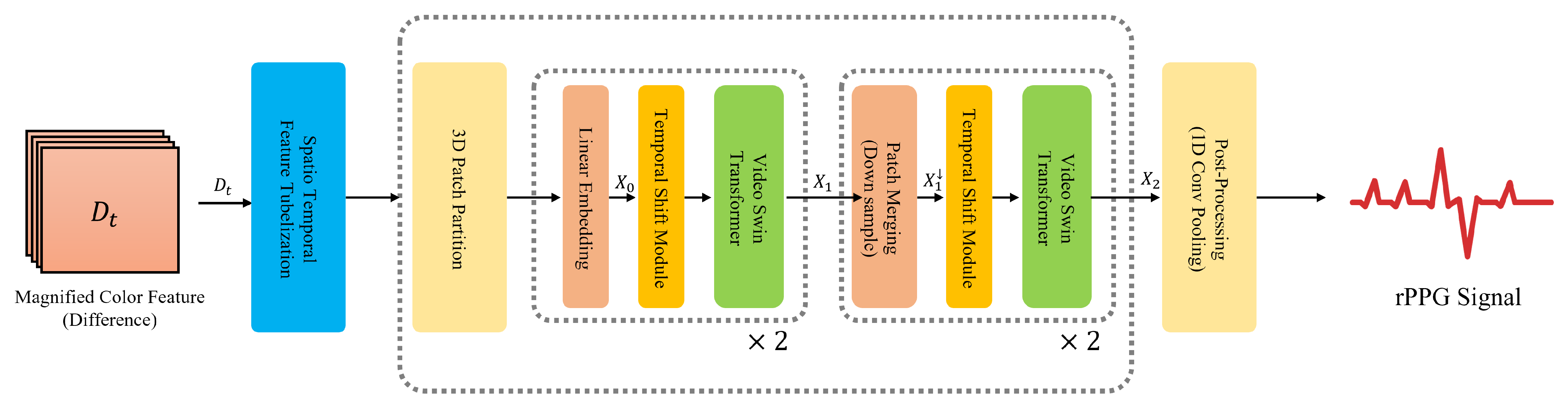
In the pipeline of this framework, the amplification process for rPPG is LVM. This module borrows the encoder–manipulator–decoder structure used in existing deep learning-based LVM methods [8] but omits the video reconstruction Decoder, which is unnecessary for rPPG signal estimation. It operates in a ‘Manipulator-Only’ fashion, extracting only the magnified features where the rPPG signal is amplified and passing them to the subsequent stages (dual-branch differencing and SSFE). The detailed structure of this VCM module is illustrated in Figure 2. This VCM module is applied with shared weights to both the face branch ( z t f ) and the background branch ( z t b ) defined in Section 3.2, similar to dual-stream concepts [15].
The feature map ( z t ) of the video to be magnified is processed through an encoder. The encoder consists of a 2D convolution layer stack, mapping the input’s raw color space features into a high-dimensional feature space where the rPPG signal and noise components are mixed, and where each feature is divided into a texture feature responsible for color and a shape feature representing motion [8]. In this paper, only the texture feature is used for rPPG.
Subsequently, before being input to the manipulator, the encoded feature sequence is received, and components only from the physiological signal band are selectively amplified in the time domain. This is implemented through a band-pass filter B θ . B θ is implemented as a 1D convolution stack, extracting only components in the HR effective band (0.7–4.0 Hz) while excluding low-frequency illumination drift and high-frequency input noise [5,6]. Afterwards, the manipulator multiplies this band-limited signal component B θ ( z ) by a scalar amplification factor α , and then performs a residual connection to the original feature z to preserve the signal of interest. The final amplification operation M θ is defined as follows:
M θ ( z ) = z + α · B θ ( z ) .

3.4. Temporal Shift Module (TSM) Injection for Spatio-Temporal Feature Extraction

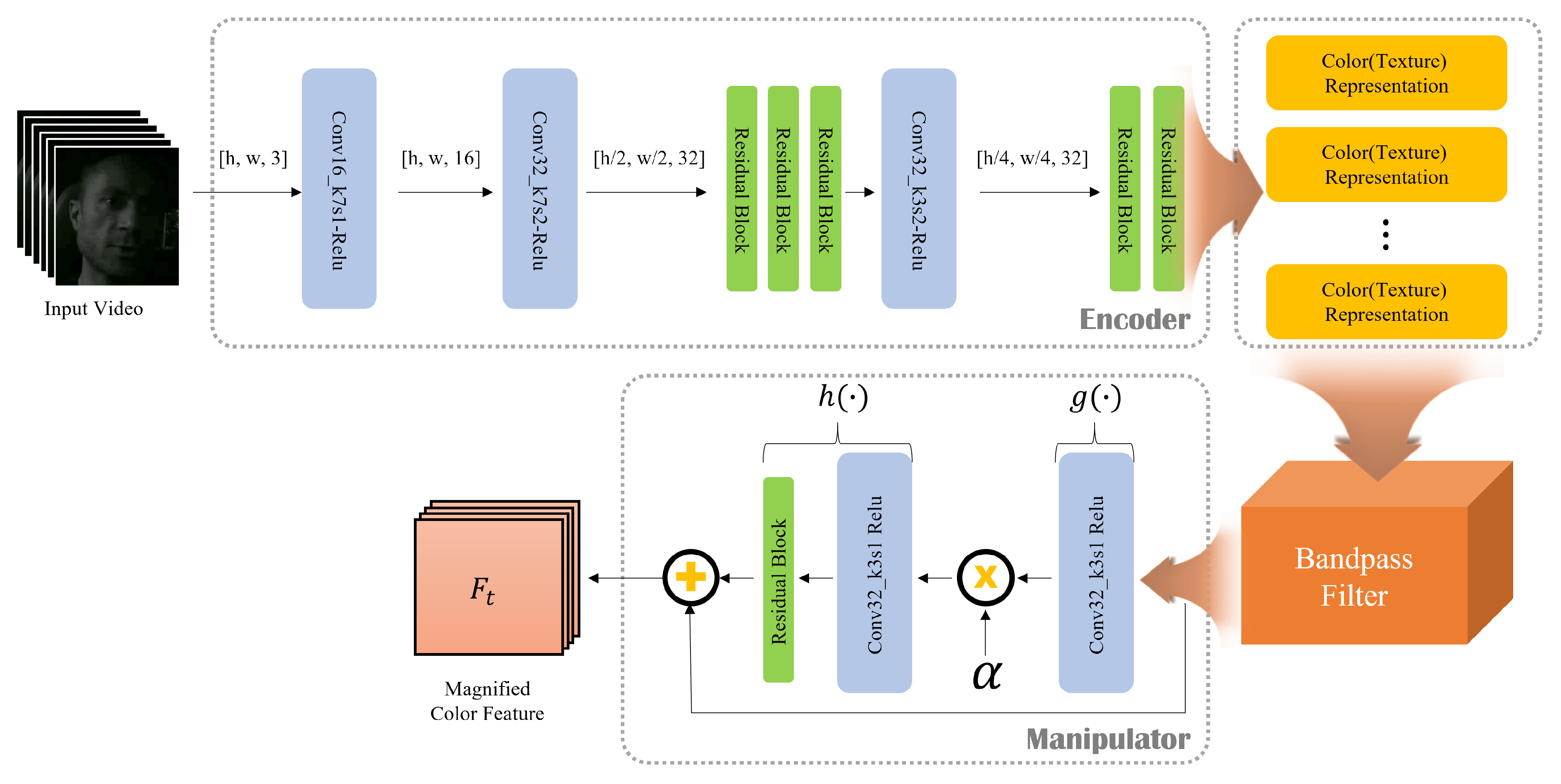
Figure 3 illustrates the architecture of the SSFE module, which is based on the TSM injection structure. To mitigate the problem where short, irregular, and impulsive movement noise in dynamic environments momentarily interferes with the low-frequency periodic signal of rPPG, we insert a TSM [16] before the window-based self-attention, which injects temporal context without increasing parameters. TSM rearranges information from adjacent time points along the channel axis, enabling each token to immediately possess information from preceding and succeeding frames [16]. This provides a virtually wider temporal receptive field without expanding the attention’s time window size.
Let the differenced magnified feature tensor obtained from the dual-branch pipeline stage be D R B × T × C × H × W . After 3D patch partitioning with size ( p t , p h , p w ) , we apply a linear embedding E d 1 to obtain:
X ( 0 ) = E d 1 Patch ( p t , p h , p w ) ( D ) R B × T × d 1 × H × W ,
where T = T / p t , H = H / p h , and W = W / p w .
The tensor U R B × T × C s × H s × W s to be fed into the Video Swin Transformer (attention block) [14] is divided into three groups along the channel axis: forward, identity, and backward:
U = U ( f ) , U ( id ) , U ( b ) , C f = r f C s , C b = r b C s , C id = C s C f C b ,
where r f , r b ( 0 , 1 ) are ratio parameters. Let the time shift interval be s N , and boundaries are handled with padding. Then, TSM at time t is
TSM ( r f , r b , s ) ( U ) t = U t s ( f ) , U t ( id ) , U t + s ( b ) R B × 1 × C s × H s × W s .
That is, it arranges the representations from time points ( t s , t , t + s ) side by side within the channels at the same spatial location, allowing the subsequent attention block to simultaneously reference past and future phase information with only a small time window [16,17].
The block at each step follows the order “TSM → window-based self-attention → MLP” [17]. Using Layer Normalization (LN), window-based self-attention (WSA), and MLP, the update in block k is given by the following:
Q = TSM LN ( X ) , X = X + WSA ( Q ) , X + = X + MLP LN ( X ) ,
where X + becomes the next input. In stage i, these blocks are repeated n i times to obtain X ( i ) , followed by a patch merging M 2 × 2 restricted to the spatial axes, changing ( H i , W i ) ( H i / 2 , W i / 2 ) and expanding the channels d i d i + 1 (the temporal length T is preserved).
The final stage output is pooled by spatial averaging and reduced to Z R B × T × d * . It then goes through a post-process stage H (using 1D convolution) to regress the rPPG waveform:
y ˜ = H ( Z ) R B × T
If necessary, y ˜ is interpolated back to the original length T to obtain y , and HR is calculated via power spectrum-based HR estimation [5,6].

4. Experimental Results

4.1. Experimental Setting

Table 1 and Table 2 present the detailed specifications of the used datasets and the hyperparameter configuration. We use two datasets with different characteristics to simultaneously verify baseline performance in static environments and robustness in real-world dynamic environments. We selected these datasets to rigorously validate the adaptability of the proposed method through a clear contrast between ‘controlled’ and ‘real-world’ environments. Table 1 shows the detailed specification of the datasets used in this study.
UBFC-rPPG [18] provides RGB facial videos filmed indoors synchronized with BVP signals. As detailed in Table 1, this dataset includes 42 subjects under low-noise studio lighting, making it suitable for evaluating the baseline of rPPG signal estimation under relatively static conditions. For the controlled UBFC-rPPG dataset, we used the Mean Squared Error (MSE) loss to precisely reconstruct the signal waveform.
MR-NIRP [3,4] provides data captured inside a vehicle with 19 subjects. It includes both ‘Stationary’ and ‘Driving’ scenarios containing various unpredictable noises such as drastic natural light changes, camera and vehicle shake, and motion blur. By using these two datasets, the algorithm’s signal estimation capability and noise robustness can be verified across clearly distinguished domains. In this study, the RGB track of MR-NIRP is used as the evaluation target. For the MR-NIRP dataset, characterized by significant noise variations, we employed the Negative Pearson Correlation loss. This loss focuses on phase alignment and periodicity, making it robust to the amplitude scaling issues caused by environmental noise. To standardize the input for the model across different datasets, we performed face detection and cropping on all video data, followed by resizing to a uniform 128 × 128 resolution.

4.2. Results

To validate the final robustness of the proposed method, we compares its performance against SOTA and standard deep learning baselines. We selected VS-Net [13] as the baseline, which was reported in its research to achieve top-tier performance on benchmarks such as UBFC-rPPG. We re-implemented the model to evaluate its performance under the specific noise conditions targeted in this study. To ensure a fair comparison, the identical preprocessing pipeline (including face detection and data preprocessing) was applied to both the UBFC-rPPG and MR-NIRP datasets. We also included representative deep learning-based rPPG methodologies: DeepPhys [24], a standard branch-based CNN model that analyzes shape and motion separately, and RhythmNet [12], which utilizes Spatio-Temporal Maps. The evaluation was performed under (1) simulated complex noise (UBFC-Both), (2) a limited real-world noise environment (MR-NIRP-Stationary), and (3) a severe real-world noise environment (MR-NIRP-Driving).
Table 3 shows the results for the ‘Both Noise’ condition on the UBFC dataset, which combines global illumination changes and irregular motion. In this controlled mixed-noise environment, the proposed model (Ours) achieved the best performance across all metrics. While the baseline VS-Net also showed strong performance, the proposed model demonstrated superior robustness through the complementary synergy of the Dual-branch pipeline and the TSM injection structure, achieving an 15.7% improvement on the MAE metric compared to VS-Net. The comparison models, DeepPhys and RhythmNet, showed significantly higher errors in the mixed-noise environment.
Table 4 shows the results for the real-world in-vehicle stationary condition. While noise is controlled in this non-driving scenario, it still contains real-world noise sources, such as engine micro-vibrations and subtle ambient light changes, that are not present in studio environments like UBFC-rPPG. In this scenario, the baseline, VS-Net, showed superior performance compared to the proposed model. This result is consistent with the original VS-Net, which reported very high accuracy in low-noise environments like UBFC-rPPG. This result clearly demonstrates the design trade-off of the proposed model. This means that the modules specialized for noise cancellation may act as an unnecessary overhead in low-noise environments, resulting in a performance penalty.
Table 5 compares the final performance in the most difficult and challenging real-world setting: the MR-NIRP ‘Driving’ scenario. This environment includes severe complex noise occurring during actual driving, such as strong illumination changes, vehicle vibrations, and road shocks.
As expected, the performance of all models degraded significantly compared to the stationary environment (Table 4). Standard CNN-based methodologies, such as DeepPhys and RhythmNet, exhibited very high error rates in terms of MAE, and their correlation R almost collapsed, practically failing to capture the signal’s correlation. This clearly demonstrates that in high-noise environments, attention-based Spatio-Temporal Feature Extracting methods (VS-Net and Ours) are vastly superior to traditional CNN methods. Nevertheless, the baseline, VS-Net, also showed a high error rate in terms of MAE, revealing its performance limitations.
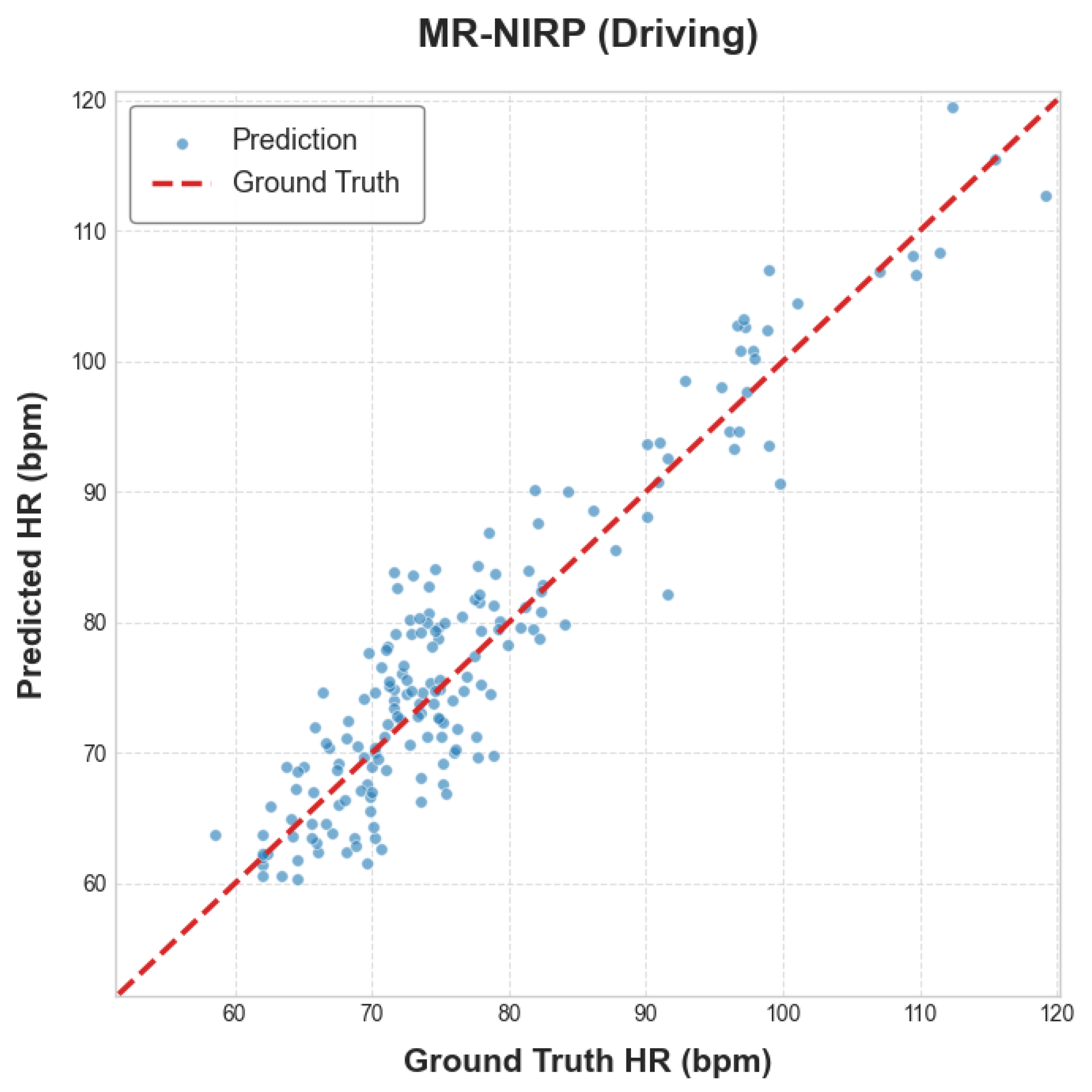
Nonetheless, the proposed model (Ours) achieved the lowest error rates in terms of MAE and RMSE, and also maintained the highest correlation R, uniquely preserving meaningful signal capture. Figure 4 presents the scatter plot of the predicted heart rates versus the ground truth for our method under this driving scenario(most noisy). The plot demonstrates a linear correlation with data points tightly clustered around the ideal regression line, confirming that our model effectively recovers the underlying physiological signal even amidst severe environmental noise. Quantitatively, this represents an approximate 13.8% improvement in MAE compared to the baseline VS-Net. This result ultimately proves that the proposed model’s complementary noise defense structure can provide the most robust and stable performance even in the harshest noise environment where all other models fail.

4.3. Ablation Study

To analyze in detail how the two key contributions of the proposed model (dual-branch pipeline, TSM injection) affect performance under each noise scenario, we conducted an ablation study. The comparison consists of (1) Ours (full model), (2) Ours (single branch) (dual-branch removed, TSM only), and (3) Ours (TSM module off) (TSM removed, dual-branch only), and includes VS-Net as the baseline. The ablation study was performed on both the four simulated conditions of the UBFC-rPPG [18] and the two real-world conditions (Stationary and Driving) of the MR-NIRP dataset [3,4]. The simulation conditions for UBFC are as follows: ‘Clean’ uses the original sequences. ‘illumination change noise’ implements global illumination change noise by adding low-frequency brightness/color component change noise to the entire frame. ‘Motion’ reproduces camera/subject jitter and motion blur by applying small-scale rotations/irregular vibrations and Gaussian/box blur on a frame-by-frame basis. ‘Both’ configures a simultaneous occurrence scenario by synthesizing the two disturbances. The parameters for each condition (modulation amplitude, frequency band, transformation/blur magnitude) are fixed within an experiment set, but their occurrence frequency and periodicity are randomly given, and the VCM amplification factor α was set to 80.
The ‘Illumination Change Noise’ condition in Table 6 clearly isolates the contribution of the dual-branch pipeline. The Ours (Full) achieved the best performance, and Ours-TSM module off (dual-branch only) also performed strongly. In stark contrast, Ours-single branch (TSM only), which lacks the dual-branch, remained at a poor performance level with an R. The single branch model’s MAE was 14.7% higher than Ours-TSM module off, demonstrating that the TSM module alone has no mechanism to remove spatial illumination change noise. This proves that the dual-branch pipeline, present in the other model, successfully canceled the global noise via the F t κ * B t operation. The 3.3% additional MAE improvement in Ours (Full) over Ours-TSM module off suggests TSM played a minor, secondary role in stabilizing residual noise after the dual-branch performed the primary cancellation.
The ‘Movement Noise’ condition in Table 7 clearly isolates the contribution of TSM, showing an opposite trend to the ‘illumination change noise’ condition. Among the ablation variants, Ours (Single Branch) (TSM only) performed significantly better than Ours (TSM module off) (dual-branch only).
The Ours (TSM module off) model, which lacked TSM, showed a much higher MAE than single branch and had the worst R. This demonstrates that TSM’s temporal smoothing function is essential for stabilizing ‘transient’ motion noise (jitter). Conversely, the dual-branch pipeline appears ineffective against local motion, or even detrimental, likely by amplifying the difference in motion. The slightly lower performance of Ours (Full) compared to single branch suggests that the benefit provided by TSM was partially offset by the penalty incurred by the dual-branch pipeline in this specific scenario.
The ‘Both Noise’ condition in Table 8 decisively demonstrates the complementary synergy of the proposed modules. While Ours (Full) (MAE 2.68) achieved the most robust performance, both ablation variants showed a significant performance collapse: Ours-single branch and Ours-TSM module off. The baseline, VS-Net performed even worse than the single branch model, recording the highest MAE.
Ours-single branch (TSM only) failed to defend against illumination change noise, resulting in an 11.6% higher MAE than Ours and a poor R. Ours-TSM module off (dual-branch only) was vulnerable to motion noise, resulting in a 2.2% higher MAE than Ours and an even lower R. This signifies that removing either key contribution leads to a failure to defend against the remaining noise type. The fact that VS-Net, which is vulnerable to both noise types, showed the worst performance suggests that only the full Ours model, with both modules combined, established a structure for responding to mixed noise to achieve a successful outcome in this complex environment.
The ‘Clean’ condition in Table 9 details the basis for the design trade-off identified in the Main Results (Table 4). While the VS-Net baseline performed best in this ideal noise-free environment, the focus of the ablation study is the comparison among the proposed variants. Among these variants, Ours-single branch (TSM only) had the lowest error. Ours-TSM module off (dual-branch only) showed a larger performance drop than using TSM alone. Ours, with both modules applied, recorded the largest error as these two penalties accumulated. This suggests that on clean signals, the TSM module introduces a minor overhead, while the dual-branch pipeline incurs a larger penalty, likely due to signal attenuation.
Table 10 presents the results for the real-world MR-NIRP Stationary condition. As already confirmed in the Main Results (Table 4), the MR-NIRP dataset is significantly more challenging than UBFC-rPPG, with MAE values exceeding 1.55 even in this ‘quasi-clean’ environment.
In this condition, the VS-Net baseline again achieved the best performance, corroborating the trend from the ‘Clean’ test (Table 9) on real-world data. The ablation results also follow the identical VS-Net > single branch > TSM module off > Ours trend. The Ours-single branch (TSM only) introduced a minor overhead with a 4.5% MAE increase over VS-Net, while the Ours-TSM module off (dual-branch pipeline only) caused a larger performance drop of 9.7%, and Ours (Full), combining both, showed the largest penalty at 14.8%. This result confirms that the proposed modules act as a trade-off in real-world environments below a certain noise threshold.
Table 11, showing results from the harshest real-world ‘Driving’ scenario, provides the final validation and perfectly reproduces the complementary synergy conclusion from ‘Both Noise’ (Table 8). Ours (Full) achieved the most robust performance, while the baseline VS-Net recorded the worst performance with a collapsed R.
Both ablation variants also suffered significant performance degradation compared to Ours (Full). Ours-single branch (TSM only) showed a 11.5% higher MAE than Ours, and Ours-TSM module off (dual-branch only) showed a 5.3% higher MAE than Ours.
This demonstrates that the complex noise of the real-world driving environment caused both single branch (failing to defend against illumination change noise) and TSM module off (failing to defend against motion) to collapse, while VS-Net, being vulnerable to both noise types, showed the greatest performance degradation. This conclusively proves that only Ours, with the combination of both modules, can maintain meaningful performance and overcome the limitations of the baseline in this severe environment.

5. Conclusions

To bridge the gap between static, studio-type benchmarks and real-world dynamic, noisy environments, this study enhanced rPPG robustness in dynamic environments, specifically modeling movement noise and illumination change noise, on top of a VS-Net series backbone through two key contributions: (1) post-VCM Foreground–Background Dual-Branch Differencing pipeline and (2) TSM module injection inside the SSFE. The proposed method showed consistent performance improvements over the VS-Net baseline under illumination change noise and Both Noise conditions on UBFC, as well as in the high-noise Driving scenario on MR-NIRP. Although the proposed method demonstrated superior robustness, a performance trade-off was observed in the noise-free (Clean) experiment, the impulsive Movement Noise experiment (UBFC), and the quasi-clean Stationary condition (MR-NIRP), where the baseline VS-Net was superior.
The ablation results support that under illumination change noise conditions, the dual-branch pipeline provides the core benefit, while under movement noise conditions, TSM provides additional gains, and the combination of both elements achieves optimal robustness in the most challenging conditions.
This structural design, while advantageous in noisy settings, introduces an inherent trade-off in low-noise environments. Specifically, the dual-branch pipeline, designed to remove ‘common’ noise, can inadvertently attenuate valid physiological signals when such noise is absent. Simultaneously, the TSM, aimed at smoothing ‘transient’ noise, may blunt the fine-grained peaks of stable signals, leading to a slight performance degradation in clean conditions. Our model accepts these penalties to secure robustness in high-noise scenarios.
However, limitations still exist. The proposed method relies on the accurate segmentation of foreground and background regions. While we mitigated sensitivity to minor alignment errors by employing the robust MTCNN [23] for landmark detection and geometric alignment, performance may still degrade in scenarios with severe occlusion or extreme poses where landmarks cannot be detected. In such cases, the separation of Ω f and Ω b may fail, leading to inaccurate rPPG estimation. Other limitations include weakness in low-light conditions and sensitivity to the quality of ROI alignment. Additionally, while the TSM effectively mitigates ‘impulsive/transient vibration’ caused by vehicle shocks, it is not designed for large-scale motion compensation.

6. Future Work

Future research will focus on systematically securing robustness through techniques such as curriculum learning, domain randomization, and worst-risk minimization to address the challenges of global illumination changes, vibrations, and blur encountered in real-world dynamic environments. Building on these foundations, we plan to strengthen the theoretical grounding of our model against geometric noise by incorporating insights from robust feature extraction in complex scenes [25,26] and strategies against geometric perturbations [27,28]. Inspired by these advancements, we aim to develop a multidimensional feature strategy that maintains invariant performance even under severe geometric attacks and complex illumination changes, thereby systematically securing rPPG robustness.
To enhance model expressiveness and fundamentally address the trade-off observed in clean environments, we will introduce adaptive mechanisms. Specifically, we aim to design the differencing weight κ * as a ‘learnable gate’ that dynamically controls the activation of the differencing operation based on the environmental noise level, thereby preventing signal attenuation in low-noise scenarios. Concurrently, we anticipate improving efficiency by implementing a reinforcement learning-based adaptive magnification factor that dynamically adjusts α based on the input video state, along with a VCM specialized for the cardiac band.
Finally, we aim to extend our validation scope to ensure generalization across diverse sensor characteristics and environments. This includes testing on a broader range of hardware conditions, such as various resolutions, frame rates, noise type, and NIR/RGB tracks, to develop a framework robust to these variations. While this study focused on proving the robustness of HR accuracy using standard metrics (MAE, RMSE, R), we plan to extend our validation to include fine-grained physiological metrics, such as Heart Rate Variability (HRV), in future research. Ultimately, our goal is to present a reliable rPPG methodology for actual vehicle environments by verifying stability across various real-vehicle scenarios, including stationary/driving, day/night, and weather changes.

Author Contributions

Conceptualization, G.C. and M.-J.K.; methodology, G.C.; software, G.C.; validation, M.-J.K. and C.W.A.; formal analysis, G.C. and M.-J.K.; investigation, G.C.; resources, C.W.A.; data curation, G.C.; writing—original draft preparation, G.C.; writing—review and editing, M.-J.K. and C.W.A.; visualization, G.C.; supervision, M.-J.K.; project administration, C.W.A.; funding acquisition, M.-J.K. and C.W.A. All authors have read and agreed to the published version of the manuscript.

Funding

This work was supported by Basic Science Research Program through the National Research Foundation of Korea (NRF) funded by the Ministry of Education(RS-2025-25398164), and the Institute of Information & communications Technology Planning & Evaluation (IITP) grant funded by the Korea government (MSIT) (No. 2019-0-01842, Artificial Intelligence Graduate School Program (GIST) & the Artificial Intelligence Convergence Innovation Human Resources Development (IITP-2023-RS-2023-00256629)), ITRC (Information Technology Research Center) support program (IITP-2025-RS-2024-00437718).

Data Availability Statement

The data presented in this study are openly available in UBFC-rPPG [18]—https://sites.google.com/view/ybenezeth/ubfcrppg (accessed on 25 November 2025), MR-NIRP [3,4]—https://computationalimaging.rice.edu/mr-nirp-dataset/ (accessed on 25 November 2025).

Conflicts of Interest

The authors declare no conflicts of interest.

References

  1. Verkruysse, W.; Svaasand, L.O.; Nelson, J.S. Remote plethysmographic imaging using ambient light. Opt. Express 2008, 16, 21434–21445. [Google Scholar] [CrossRef] [PubMed]
  2. Poh, M.Z.; McDuff, D.J.; Picard, R.W. Non-contact, automated cardiac pulse measurements using video imaging and blind source separation. Opt. Express 2010, 18, 10762–10774. [Google Scholar] [CrossRef] [PubMed]
  3. Nowara, E.M.; Marks, T.K.; Mansour, H.; Veeraraghavan, A. Near-Infrared Imaging Photoplethysmography During Driving. IEEE Trans. Intell. Transp. Syst. 2020, 23, 21320–21330. [Google Scholar] [CrossRef]
  4. Nowara, E.M.; Marks, T.K.; Mansour, H.; Veeraraghavan, A. SparsePPG: Towards Driver Monitoring Using Camera-Based Vital Signs Estimation in Near-Infrared. In Proceedings of the IEEE/CVF International Conference on Computer Vision Workshops (ICCVW), Montreal, QC, Canada, 10–17 October 2021. [Google Scholar]
  5. De Haan, G.; Jeanne, V. Robust pulse rate from chrominance-based rPPG. IEEE Trans. Biomed. Eng. 2013, 60, 2878–2886. [Google Scholar] [CrossRef] [PubMed]
  6. Wang, W.; den Brinker, A.C.; Stuijk, S.; de Haan, G. Algorithmic Principles of Remote PPG. IEEE Trans. Biomed. Eng. 2016, 64, 1479–1491. [Google Scholar] [CrossRef] [PubMed]
  7. Wu, H.Y.; Rubinstein, M.; Shih, E.; Guttag, J.; Durand, F.; Freeman, W. Eulerian Video Magnification for Revealing Subtle Changes in the World. ACM Trans. Graph. 2012, 31, 1–8. [Google Scholar] [CrossRef]
  8. Oh, T.H.; Jaroensri, R.; Kim, C.; Elgharib, M.; Durand, F.; Freeman, W.T.; Matusik, W. Learning-based Video Motion Magnification. In Proceedings of the European Conference on Computer Vision (ECCV), Munich, Germany, 8–14 September 2018; pp. 633–648. [Google Scholar]
  9. Tran, D.; Bourdev, L.; Fergus, R.; Torresani, L.; Paluri, M. Learning Spatiotemporal Features with 3D Convolutional Networks (C3D). In Proceedings of the IEEE International Conference on Computer Vision (ICCV), Santiago, Chile, 7–13 December 2015; pp. 4489–4497. [Google Scholar]
  10. Carreira, J.; Zisserman, A. Quo Vadis, Action Recognition? A New Model and the Kinetics Dataset (I3D). In Proceedings of the IEEE Conference on Computer Vision and Pattern Recognition (CVPR), Honolulu, HI, USA, 21–26 July 2017; pp. 6299–6308. [Google Scholar]
  11. Feichtenhofer, C.; Fan, H.; Malik, J.; He, K. SlowFast Networks for Video Recognition. In Proceedings of the IEEE/CVF International Conference on Computer Vision (ICCV), Seoul, Republic of Korea, 27 October–2 November 2019; pp. 6202–6211. [Google Scholar]
  12. Niu, X.; Han, H.; Shan, S.; Chen, X. RhythmNet: End-to-End Heart Rate Estimation from Face via Spatial-Temporal Representation. IEEE Trans. Image Process. 2019, 29, 2409–2423. [Google Scholar] [CrossRef] [PubMed]
  13. Sun, N.; He, P.; Liu, J.; Chai, L.; Wu, C.; Liu, X. Remote heart rate measurement based on video color magnification and spatiotemporal self-attention. Biomed. Signal Process. Control 2025, 106, 107677. [Google Scholar] [CrossRef]
  14. Liu, Z.; Ning, J.; Cao, Y.; Wei, Y.; Zhang, Z.; Lin, S.; Hu, H. Video Swin Transformer. In Proceedings of the IEEE/CVF Conference on Computer Vision and Pattern Recognition (CVPR), New Orleans, LA, USA, 19–24 June 2022; pp. 3202–3211. [Google Scholar]
  15. Kang, J.; Yang, S.; Zhang, W. TransPPG: Two-stream Transformer for Remote Heart Rate Estimate. CCF Trans. Pervasive Comput. Interact. 2024, 6, 271–280. [Google Scholar] [CrossRef]
  16. Lin, J.; Gan, C.; Han, S. TSM: Temporal Shift Module for Efficient Video Understanding. In Proceedings of the IEEE/CVF International Conference on Computer Vision (ICCV), Seoul, Republic of Korea, 27 October–2 November 2019; pp. 7083–7093. [Google Scholar]
  17. Liu, X.; Fromm, J.; Patel, S.; McDuff, D. Multi-Task Temporal Shift Attention Networks for On-Device Contactless Vitals Measurement. In Proceedings of the 34th Conference on Neural Information Processing Systems (NeurIPS), Vancouver, BC, Canada, 6–12 December 2020. [Google Scholar]
  18. Bobbia, S.; Macwan, R.; Benezeth, Y.; Mansouri, A.; Dubois, J. Unsupervised skin tissue segmentation for remote photoplethysmography. Pattern Recognit. Lett. 2019, 124, 82–90. [Google Scholar] [CrossRef]
  19. Qiu, Y.; Liu, Y.; Arteaga-Falconi, J.; Ghasemzadeh, H. EVM-CNN: Real-time contactless heart rate estimation from facial video. IEEE Trans. Multimed. 2018, 21, 1778–1787. [Google Scholar] [CrossRef]
  20. Liu, Z.; Lin, Y.; Cao, Y.; Hu, H.; Wei, Y.; Zhang, Z.; Lin, S.; Guo, B. Swin Transformer: Hierarchical Vision Transformer using Shifted Windows. In Proceedings of the IEEE/CVF International Conference on Computer Vision (ICCV), Montreal, QC, Canada, 10–17 October 2021; pp. 10012–10022. [Google Scholar]
  21. Gideon, J.; Stent, S. The Way to My Heart is Through Contrastive Learning: Remote Photoplethysmography from Unlabelled Video. In Proceedings of the IEEE/CVF International Conference on Computer Vision (ICCV), Montreal, QC, Canada, 10–17 October 2021; pp. 3995–4004. [Google Scholar]
  22. Li, Z.; Li, B.; Yin, L. Contactless Pulse Estimation Leveraging Pseudo Labels and Self-Supervision. In Proceedings of the IEEE/CVF International Conference on Computer Vision (ICCV), Paris, France, 2–6 October 2023; pp. 20588–20597. [Google Scholar]
  23. Zhang, K.; Zhang, Z.; Li, Z.; Qiao, Y. Joint Face Detection and Alignment using Multi-task Cascaded Convolutional Networks (MTCNN). IEEE Signal Process. Lett. 2016, 23, 1499–1503. [Google Scholar] [CrossRef]
  24. Chen, W.; McDuff, D. DeepPhys: Video-Based Physiological Measurement Using Convolutional Attention Networks. In Proceedings of the European Conference on Computer Vision (ECCV), Munich, Germany, 8–14 September 2018; pp. 349–365. [Google Scholar]
  25. Liu, Y.; Wang, C.; Lu, M.; Yang, J.; Gui, J.; Zhang, S. From Simple to Complex Scenes: Learning Robust Feature Representations for Accurate Human Parsing. IEEE Trans. Pattern Anal. Mach. Intell. 2024, 46, 5449–5462. [Google Scholar] [CrossRef]
  26. Sun, G.; Wang, C.; Hua, Y. Spatio-temporal Prompting Network for Robust Video Feature Extraction. In Proceedings of the IEEE/CVF International Conference on Computer Vision (ICCV), Paris, France, 2–6 October 2023. [Google Scholar]
  27. Wang, C.; Zhang, Q.; Wang, X.; Zhou, L.; Li, Q.; Xia, Z.; Ma, B.; Shi, Y. Light-Field Image Multiple Reversible Robust Watermarking Against Geometric Attacks. IEEE Trans. Dependable Secur. Comput. 2025, 22, 5861–5875. [Google Scholar] [CrossRef]
  28. Jiang, Y.; Chiang, H.D. Geometry-Aware Weight Perturbation for Adversarial Training. Electronics 2024, 13, 3508. [Google Scholar] [CrossRef]
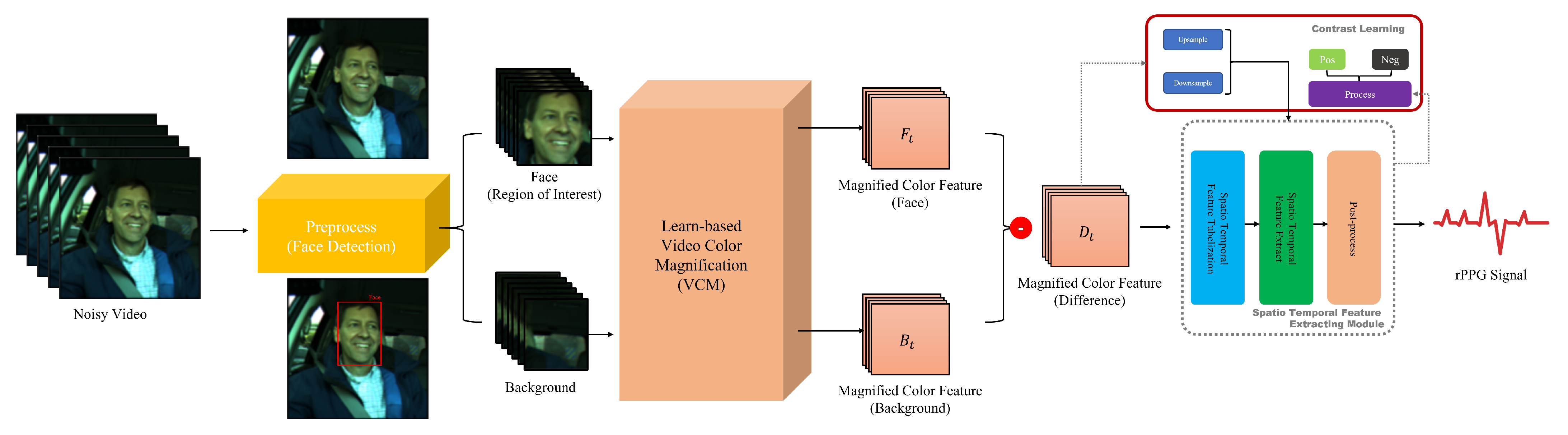
Figure 1. Overview of the proposed dualbBranch differencing pipeline. The input video is preprocessed to separate face (Region of Interest) and background streams. A shared-weight Video Color Magnification (VCM) module amplifies both streams to produce F t (Face) and B t (Background). Global noise is canceled by subtracting the adaptively scaled background feature from the face feature ( D t = F t κ * B t ). This noise-robust feature D t is then passed to the Spatio-Temporal Feature Extracting Module for final rPPG signal estimation.
Mathematics 13 03830 g001
Figure 2. Architecture of the Learn-based Video Color Magnification (VCM) module. The encoder (top) uses a stack of 2D convolutions and residual blocks to extract the Color (Texture) Representation, z . This feature z splits: one path provides the residual connection for the final addition (+). The other path is fed into the band-pass filter to isolate the physiological signal, which is then processed by the manipulator (bottom). The manipulator scales the signal by a amplified factor α and refines it through convolutional and residual blocks. Finally, this amplified path is added back to the original feature z to produce the Magnified Color Feature F t .
Mathematics 13 03830 g002
Figure 3. The architecture of the Spatio-Temporal Feature Extracting (SSFE) module, modified with TSM injection. The input differenced feature D t is processed by Feature Tubelization and 3D Patch Partition. The resulting tokens are fed into two stages, each comprising a Temporal Shift Module (TSM) placed immediately before a Video Swin Transformer block. A Post-Processing block regresses the final rPPG signal.
Mathematics 13 03830 g003
Figure 4. Scatter plot of predicted HR vs. Ground Truth HR for “Ours” on the MR-NIRP (Driving) dataset.
Mathematics 13 03830 g004
Table 1. Detailed specifications of the datasets used in this study. UBFC-rPPG represents a controlled indoor environment, while MR-NIRP represents a challenging real-world in-vehicle environment.
FeatureUBFC-rPPG [18]MR-NIRP [3,4]
EnvironmentIndoor (Controlled)In-vehicle (Real-world)
Subjects42 peoples (30 Male, 12 Female)19 peoples (17 Male, 2 Female)
Resolution 640 × 480 pixels 640 × 640 pixels
Frame Rate30 fps30 fps
ConditionsLow-noise studio lightingStationary & Driving
Noise FactorsMinimalNatural light, Tunnels, Vibration
Table 2. Detailed hyperparameter configuration.
ParameterValue
OptimizerAdam
Learning Rate (LR) 1 × 10 4
Batch Size4
Num Epochs80
VCM Amplification ( α )80
TSM Shift Ratio ( r f , r b )1/8
Loss FunctionMSE (UBFC-rPPG), Neg. Pearson (MR-NIRP)
Table 3. Main results on UBFC-rPPG with Both Noise. Comparison against standard deep learning baselines (DeepPhys, RhythmNet) and the SOTA baseline (VS-Net). Lower is better for MAE/RMSE; higher is better for R.
MetricDeepPhys [24]RhythmNet [12]VS-Net (Baseline) [13]Ours
MAE (bpm) ↓4.714.523.182.68
RMSE (bpm) ↓6.266.084.123.62
R0.6930.6800.8180.845
Table 4. Main results on MR-NIRP (Stationary). Comparison against standard deep learning baselines (DeepPhys, RhythmNet) and the SOTA baseline (VS-Net). Lower is better for MAE/RMSE; higher is better for R.
MetricDeepPhys [24]RhythmNet [12]VS-Net (Baseline) [13]Ours
MAE (bpm) ↓3.182.871.551.78
RMSE (bpm) ↓4.774.612.682.89
R0.7210.8340.9110.893
Table 5. Main results on MR-NIRP (Driving). Comparison against standard deep learning baselines (DeepPhys, RhythmNet) and the SOTA baseline (VS-Net). Lower is better for MAE/RMSE; higher is better for R.
MetricDeepPhys [24]RhythmNet [12]VS-Net (Baseline) [13]Ours
MAE (bpm) ↓13.2611.534.353.75
RMSE (bpm) ↓17.9215.038.127.02
R0.4320.4710.7240.803
Table 6. Illumination change noise (UBFC-rPPG with Illumination Change Noise). Comparison of VS-Net, our method (dual-branch pipeline + TSM), and ablations (single branch: dual-branch differencing removed; TSM off: temporal shift removed). Lower is better for MAE/RMSE; higher is better for R.
MetricVS-NetOursOurs-Single BranchOurs-TSM Module Off
MAE (bpm) ↓2.832.372.812.45
RMSE (bpm) ↓3.763.124.053.38
R0.8510.9120.8690.895
Table 7. Movement (UBFC-rPPG with Movement Noise). Comparison of VS-Net, our method (dual-branch pipeline + TSM), and ablations (single branch: dual-branch differencing removed; TSM off: temporal shift removed). Lower is better for MAE/RMSE; higher is better for R.
MetricVS-NetOursOurs-Single BranchOurs-TSM Module Off
MAE (bpm) ↓2.362.512.452.79
RMSE (bpm) ↓3.413.683.593.95
R0.8820.8650.8740.841
Table 8. Both (UBFC-rPPG with Both Noise). Comparison of VS-Net, our method (dual-branch pipeline + TSM), and ablations (single branch: dual-branch differencing removed; TSM off: temporal shift removed). Lower is better for MAE/RMSE; higher is better for R.
MetricVS-NetOursOurs-Single BranchOurs-TSM Module Off
MAE (bpm) ↓3.182.682.992.74
RMSE (bpm) ↓4.123.624.073.83
R0.8180.8450.8250.838
Table 9. Clean (original UBFC-rPPG). Comparison of VS-Net, our method (dual-branch pipeline + TSM), and ablations (single branch: dual-branch differencing removed; TSM off: temporal shift removed). Lower is better for MAE/RMSE; higher is better for R.
MetricVS-NetOursOurs-Single BranchOurs-TSM Module Off
MAE (bpm) ↓0.821.471.051.28
RMSE (bpm) ↓1.121.981.451.76
R0.9980.9900.9950.993
Table 10. MR-NIRP (in-vehicle, stationary). Comparison of VS-Net, our method (dual-branch pipeline + TSM), and ablations (single branch: dual-branch differencing removed; TSM off: temporal shift removed). Lower is better for MAE/RMSE; higher is better for R.
MetricVS-NetOursOurs-Single BranchOurs-TSM Module Off
MAE (bpm) ↓1.551.781.621.70
RMSE (bpm) ↓2.682.892.752.83
R0.9110.8930.9050.901
Table 11. MR-NIRP (in-vehicle, driving). Comparison of VS-Net, our method (dual-branch pipeline + TSM), and ablations (single branch: dual-branch differencing removed; TSM off: temporal shift removed). Lower is better for MAE/RMSE; higher is better for R.
MetricVS-NetOursOurs-Single BranchOurs-TSM Module Off
MAE (bpm) ↓4.353.754.183.95
RMSE (bpm) ↓8.127.027.867.41
R0.7240.8030.7510.782
Disclaimer/Publisher’s Note: The statements, opinions and data contained in all publications are solely those of the individual author(s) and contributor(s) and not of MDPI and/or the editor(s). MDPI and/or the editor(s) disclaim responsibility for any injury to people or property resulting from any ideas, methods, instructions or products referred to in the content.