Dynamics of Soliton Solutions to Nonlinear Coupled System with Neural Network and Chaotic Insights

Abstract

This study examines the nonlinear dynamical behavior of a Van der Waals system in the viscosity–capillarity regularization form. The solitary wave solutions of the proposed model are investigated using advanced analytical techniques, including the generalized Arnous method, the modified generalized Riccati equation mapping method, and the modified F-expansion approach. Additionally, we use mathematical simulations to enhance our comprehension of wave propagation. Moreover, a machine learning algorithm known as the multilayer perceptron regressor neural network was adopted to predict the performance results of our soliton solutions. Another important aspect of this study is the exploration of the chaos of the studied model by introducing a perturbed system. Chaotic analysis is supported by different techniques, such as return maps, power spectra, a bifurcation diagram, and a chaotic attractor. This multifaceted investigation not only emphasizes the rich dynamical pattern of the studied model but also presents a robust mathematical framework for studying nonlinear systems. The studied model also presents a robust mathematical framework for studying nonlinear systems. This study offers novel insights into nonlinear dynamics and wave phenomena by assessing the effectiveness of modern methodologies and clarifying the distinctive characteristics of a system’s nonlinear dynamics.

1. Introduction

Nonlinear partial differential equations (NLPDEs) play a vital role in thermodynamics, governing how quantities such as pressure, temperature, and velocity evolve within fluids and gases. These equations form the foundation for modeling thermodynamic behavior, where properties like internal energy and enthalpy, essential for calculating heat and work in industrial processes, are not directly measurable but can be inferred by solving NLPDEs that incorporate conservation laws and material relations. Despite their importance, the nonlinear nature of these equations poses major analytical and numerical challenges. Considerable research has been devoted to finding exact and approximate solutions, yet many problems remain unresolved due to the complex, high-order structure of NLPDEs [1,2]. They describe the spatial and temporal evolution of key physical variables such as temperature, displacement, and wave functions, making them indispensable for understanding real-world systems. However, their inherent complexity often prevents the derivation of straightforward analytical solutions [3]. In recent years, NLPDEs have gained increased attention for their applications in diverse fields, including electrical circuits, control theory, and wave propagation areas deeply rooted in nonlinear physical processes [4]. Obtaining analytical solutions to these equations not only clarifies the underlying mechanisms of nonlinear phenomena but also offers valuable insight for future theoretical developments. A solid grasp of nonlinear science is therefore essential for interpreting complex systems characterized by non-proportional and dynamic relationships [5,6].

Solitons are very important for simulating wave behavior in nonlinear and dispersive media in numerous fields of science due to their exceptional stability and particle-like behavior in nonlinear systems. In the fields of applied mathematics and mathematical physics, solitons are occasionally employed to depict phenomena such as plasma waves, fiber optic pulses, and waves in shallow water. They play an essential role in engineering and technology. Soliton solutions of NLPDEs are highly significant in mathematical physics due to their deep connection with nonlinear wave phenomena, field theory, and integrable systems [7]. Understanding the role of nonlinear dynamics in complicated physical systems is greatly aided by these solutions since they are accurate, stable, and constrained. In the field of mathematical physics, solitons are not only distinct phenomena; they often represent the fundamental behaviors of objects in various models. The capacity of waves to preserve their form and energy after interactions with other waves makes nonlinear dynamics and wave propagation significant subjects of study across several fields [8,9,10]. Solitons have many technical uses, including optical coupling devices, controllers, sensors, and magneto-optic waveguide structures [11,12,13]. The soliton solutions of the Van der Waals equation are of considerable significance for both theoretical and practical research in mathematical physics [14].

A more profound comprehension of physical behavior is facilitated by the development of exact solutions for a diverse array of physical processes. Because they establish the foundation for further investigation. The behavior of a physical system is usually described using ordinary or partial differential equations, which help in finding analytical or approximate solutions. PDEs serve as a powerful mathematical framework for representing complex processes in nature and industry. Numerous researchers have devised alternative approaches to address these challenges. A variety of techniques have been employed over the years: the truncated Painlevé technique [15], Hamiltonian analysis [16], the improved generalized exponential rational function [17], the Adomian decomposition technique [18], sensitivity analysis [19], Darboux transformation [20], the Bernoulli ${\displaystyle \frac{G^{\prime }}{G}}$-expansion method [21], the modified Sardar sub-equation method [22], the compact difference method [23], the ${\displaystyle \frac{G^{\prime }}{G}}$-expansion method [24], quasi-linear and monotone iterative methods [25], the Riccati equation mapping method [26], bifurcation analysis [27], neural networks [28], etc.

This study examines the nonlinear dynamics of soliton solutions of Van der Waals gas systems, acknowledging their important applications in numerous fields when dealing with real gases, especially at high pressures and low temperatures, where deviations from the ideal behavior become significant. To identify and simulate the nonlinear behaviors of the proposed model, we apply advanced integration techniques, including the generalized Arnous method [29], the modified F-expansion method [30], and the modified generalized Riccati equation method [31]. Furthermore, we utilize the multilayer perceptron regressor neural network algorithm, a neural network-based model [32], to predict outcomes based on actual analytical data. Machine learning is used to improve task performance without dependence on explicitly coded instructions, enabling computers to learn from and anticipate patterns in information. Machine learning encompasses a variety of fields, including supervised learning, unsupervised learning, and reinforcement learning. This research focuses on supervised learning, which entails training a model using labeled data. The dataset is partitioned into training and testing subsets to assess the model’s prediction efficacy. More importantly, the research extends further mathematical derivations by conducting comprehensive chaos analysis, using tools such as return maps, bifurcation diagrams, power spectra, and chaotic attractors to thoroughly examine the system’s dynamical structure. This comprehensive approach enhances the theoretical understanding of nonlinear discrete electrical lattices and provides a solid basis for future research on their control, stability, and application in engineering systems. The results demonstrate the suitability and applicability of the methodologies employed, which are important tools with significant implications for the scientific and engineering fields. These methodologies achieve substantial results that contribute to the advancement of numerous scientific disciplines and enable the development of innovative waveforms and solitons.

The remaining sections of this paper are delineated as follows: Section 2 outlines the governing mathematical model. Soliton solutions are derived in Section 3 using the mGREM, the modified F-expansion method, and the generalized Arnous method. Section 4 provides a comprehensive elucidation of the graphical depiction of several solutions. The machine learning application is presented in Section 5, the chaotic analysis is discussed in Section 6, and the conclusion is provided in Section 7.

2. The Governing Equation

Well-known Dutch physicist Johannes Diderik Van der Waals developed the Van der Waals equation in 1873 to deal with the Ideal Gas Law’s limitations in explaining how real gases behave. He believed that the equation more accurately described the physical state of real gases and therefore became a key part of the study of fluid dynamics and compressible fluids. Systems of conservation laws combining hyperbolic and elliptic features can be used to explain a wide variety of physical phenomena, but there has been a lot of theoretical discussion about hybrid systems and their applications in various works [33,34]. In this work, we study the nonlinear dynamic behavior of the Van der Waals gas system [35,36,37,38], read as

$$\begin{array}{c}\hfill U_t+{\left(P\left(V\right)\right)}_x=\beta U_{xx}-\varrho {\beta }^2{U}_{xxx}\mathrm{and}{V}_t-U_x=0,\end{array}$$

(1)

where $P,U,$ and V represent pressure, velocity, and specific volume, respectively. In addition, $\beta >0$ denotes the viscosity, where $\varrho {\beta }^2$ stands for the interfacial capillarity coefficient. The structure of the function $P\left(V\right)=V-V^3,$ is similar to that of Van der Waals, as stated in [39]. The one-dimensional longitudinal isothermal motion in elastic bars or fluids is described by the P-system in Equation (1). The corresponding eigenvalues are $\pm \sqrt{-P^{\prime }\left(V\right)}$. The system is a mixed hyperbolic–elliptic type for certain material models, as the constitutive pressure function may not be monotone.

Moreover, the proposed model has been analyzed in the literature using various approaches. In [35], sensitivity analysis and bifurcation analysis were conducted, invesitgating multistability and chaotic behavior, while the exact solutions were obtained in [36] through the use of the exponential expansion method. Similarly, in [37], the $(G^{\prime }/G^2)$ expansion and advance $e^{-\varphi \left(\zeta \right)}$-expansion function approaches were applied to secure a variety of solutions, where in [38], Kudryashov’s technique, the Sine-Gordon equation, and the Projective Riccati equation were employed to study the proposed system. This study uses new advanced techniques to examine the exact solution of the proposed model to gain a deeper understanding of its nonlinear behavior.

3. Methodology

The literature recently identified a variety of mathematical methods with which to investigate soliton dynamics in nonlinear models. This work examines the soliton solutions of the proposed model, building on previous research in soliton theory and employing advanced methods, including the generalized Arnous method, the modified F-expansion method, and the mGREM, as well as the multilayer perceptron regressor neural network. This section highlights how these methodologies are applied in real-world scientific problems to investigate the soliton solutions of the NLPDE.

$$S(g,g_t,g_{n_1},g_{n_2},g{g}_{n_1},\dots )=0,$$

(2)

where $g=g(t,n_1,n_2,\dots ,n_r).$ To solve problem (2), the following procedures are enacted. The first step is to apply wave transformation such as $g(t,n_1,n_2,\dots ,n_r)=Q\left(\xi \right)$, which is performed first, where $\xi$ can be defined with different forms. This process changes Equation (2) into the following ODE:

$$R(Q,Q^{\prime },Q{Q}^{\prime },\dots )=0,$$

(3)

where $Q^{\prime }={\displaystyle \frac{dQ}{d\xi }}.$ Sometimes, the ODE can be adapted to the homogeneous balancing criterion by integrating Equation (3).

3.1. Generalized Arnous Method

In this subsection, we summarize the main steps of the generalized Arnous method [29] for the exact solutions of Equation (2).

• Step-1: In general, the solution of Equation (3) is written in the following form:

  $$Q\left(\xi \right)=c_0+\sum _{r=1}^N{\displaystyle \frac{c_r}{{\left(\Delta \left(\xi \right)\right)}^r}}+\sum _{r=1}^N{\displaystyle \frac{{\gamma }_r{\left({\Delta }^{\prime }\left(\xi \right)\right)}^r}{{\left(\Delta \left(\xi \right)\right)}^r}},$$

  (4)

  where $c_0,c_r,$ and ${\gamma }_r$ are constants with $r=(1,2,3,\cdots ,N)$ such that N is the homogeneous balance number, and the function $\Delta \left(\xi \right)$ is determined by the following relationship:

  $${\left({\Delta }^{\prime }\left(\xi \right)\right)}^2=\left(\Delta {\left(\xi \right)}^2-\rho \right)ln{\left(\delta \right)}^2,$$

  (5)

  with

  $${\Delta }^{\left(n\right)}\left(\xi \right)=\left\{\begin{array}{c}ln{\left(\delta \right)}^{n-1}{\Delta }^{\prime }\left(\xi \right),n\mathrm{is}\mathrm{odd},\hfill \\ ln{\left(\delta \right)}^n\Delta \left(\xi \right),n\mathrm{is}\mathrm{even},\hfill \end{array}\right.$$

  for $n\ge 2$, $\delta >0,$ and $\delta \ne 1$. A solution to Equation (4) is outlined below:

  $$\Delta \left(\xi \right)={\displaystyle \frac{\rho }{4Sln\left(\delta \right){\delta }^{\xi }}}+Sln\left(\delta \right){\delta }^{\xi },$$

  (6)

  where S and $\rho$ are arbitrarily constants.
• Step-2: In Equation (3), substitute the presumed solution from Step-1, which results in the polynomial ${\displaystyle \frac{1}{\Delta \left(\xi \right)}}\left({\displaystyle \frac{{\Delta }^{\prime }\left(\xi \right)}{\Delta \left(\xi \right)}}\right).$ Next, by equating the coefficients of the same powers in the polynomial ${\displaystyle \frac{1}{\Delta \left(\xi \right)}}\left({\displaystyle \frac{{\Delta }^{\prime }\left(\xi \right)}{\Delta \left(\xi \right)}}\right),$ we obtain a system of equations. Then, by solving $c_0,c_r,{\gamma }_r$ for Equation (4), we secure the exact solutions for the desired system.

3.2. Modified F-Expansion Technique

This subsection outlines the essential steps of the modified F-expansion technique [30] as follows:

• Step-1: The following represents the solution of Equation (3):

  $$Q\left(\xi \right)={\lambda }_0+\sum _{j=1}^N{\lambda }_j{\left(\Delta \left(\xi \right)\right)}^j+\sum _{j=1}^N{\sigma }_j{\displaystyle \frac{1}{{\left(\Delta \left(\xi \right)\right)}^j}},$$

  (7)

  where

  $${\Delta }^{\prime }\left(\xi \right)={\delta }_0+{\delta }_1\Delta \left(\xi \right)+{\delta }_2\Delta {\left(\xi \right)}^2.$$

  (8)

  where ${\delta }_0,{\delta }_1,$ and ${\delta }_2$ are constants to be found later on, and the balancing principle may be used to calculate N.
• Step-2: The solutions of different kinds, together with their particular conditions, may be derived for different cases, as given in [30].
• Step-3: A polynomial equation is derived by substituting Equations (7) and (8) into Equation (3). A system of algebraic equations is derived by equating each coefficient of the polynomial to zero.
• Step-4: Utilizing computational tools, we resolve the system obtained in Step-3 and determine the values of the unknown parameters, thus potentially deriving the exact solutions.

3.3. Modified Generalized Riccati Equation Mapping Method

In general, the solution to mGREM is written as

$$\Phi \left(\xi \right)={\sigma }_0+\sum _{j=1}^N{\sigma }_j{\Omega }^j\left(\xi \right)+\sum _{j=1}^N{\nu }_j\left(\xi \right){\left({\displaystyle \frac{{\Omega }^{\prime }\left(\xi \right)}{\Omega \left(\xi \right)}}\right)}^j.$$

(9)

where ${\Omega }^{\prime }\left(\xi \right)=l_2\Omega {\left(\xi \right)}^2+l_1\Omega \left(\xi \right)+l_0$. More details of the various families of the proposed method can be found in [31].

3.4. Multilayer Perceptron Regressor Neural Network

A multilayer perceptron (MLP) regressor neural network, consisting of an input layer, an output layer, and multiple hidden layers (two hidden layers, where the first hidden layer contains 32 neurons and the second hidden layer contains 16 neurons) was applied to observe the accuracy of the obtained soliton solutions. The machine learning model was developed and trained with the assistance of computer language Python 3.13.0 obtained from https://www.python.org/downloads/release/python-3130/ (accessed on 7 October 2024). To evaluate performance, the mean squared error (MSE) was adopted as the loss function to quantify the difference between the actual and predicted outputs. The dataset was partitioned into 80 percent training and 20 percent testing data, with normalization applied to scale all input features within the range [0, 1]. The network operated through forward propagation and backward propagation processes, employing the sigmoid activation function and gradient descent optimization. A fixed learning rate of 0.1 was adopted, and the model was trained for up to 10,000 epochs to ensure convergence and accuracy.

4. Results and Discussion

4.1. Presentation of the Analytical Soliton Solutions

For solving Equation (1), consider the transformation defined as

$$U(x,t)=\Psi \left(\xi \right)V(x,t)=\Phi \left(\xi \right),\mathrm{with},\xi =a(x-\alpha t),$$

(10)

where $\alpha$ is the wave speed, and a is an arbitrary constant. By applying the transformation defined in Equation (10) into Equation (1), we get

$$\begin{array}{c}\hfill -ck{\Psi }^{\prime }\left(\xi \right)+{\beta }^2{k}^3\varrho {\Psi }^{\left(3\right)}\left(\xi \right)-\beta k^2{\Psi }^{″}\left(\xi \right)-3k\Phi {\left(\xi \right)}^2{\Phi }^{\prime }\left(\xi \right)+k{\Phi }^{\prime }\left(\xi \right)=0,\\ \hfill -ck{\Psi }^{\prime }\left(\xi \right)-k{\Phi }^{\prime }\left(\xi \right)=0.\end{array}$$

(11)

Integrating Equation (11) with zero integration constants results in

$$\begin{array}{c}\hfill -c\Psi \left(\xi \right)+\beta k\left(\beta k\varrho {\Psi }^{″}\left(\xi \right)-{\Psi }^{\prime }\left(\xi \right)\right)-\Phi {\left(\xi \right)}^3+\Phi \left(\xi \right)=0,\end{array}$$

(12)

$$\begin{array}{c}\hfill c\Phi \left(\xi \right)+\Psi \left(\xi \right)=0.\end{array}$$

(13)

Inserting $\Psi \left(\xi \right)=-c\Phi \left(\xi \right)$ in Equation (12) yields

$$-a^2\alpha {\beta }^2\varrho {\Phi }^{″}\left(\xi \right)+a\alpha \beta {\Phi }^{\prime }\left(\xi \right)+\left({\alpha }^2+1\right)\Phi \left(\xi \right)-\Phi {\left(\xi \right)}^3=0.$$

(14)

Now, applying the homogeneous balance principle between the terms ${\Phi }^3$ and ${\Phi }^{″}$ in Equation (14) gives $N=1$.

4.2. Application of Generalized Arnous Method

The solution for the generalized Arnous approach [29] may be stated as

$$\Phi \left(\zeta \right)={\sigma }_0+\sum _{r=1}^N{\displaystyle \frac{{\sigma }_r}{{\left(\Theta \left(\zeta \right)\right)}^r}}+\sum _{r=1}^N{\displaystyle \frac{{\nu }_r{\left({\Theta }^{\prime }\left(\zeta \right)\right)}^r}{{\left(\Theta \left(\zeta \right)\right)}^r}}.$$

(15)

With $N=1$, Equation (15) can be written as

$$\Phi \left(\xi \right)={\sigma }_0+{\displaystyle \frac{{\sigma }_1}{\Theta \left(\xi \right)}}+{\displaystyle \frac{{\nu }_1{\Theta }^{\prime }\left(\xi \right)}{\Theta \left(\xi \right)}}.$$

(16)

The function $\Theta \left(\xi \right)$ is defined by the following relation, with constants ${\sigma }_0,{\sigma }_1,$ and ${\nu }_1$ to be specified later:

$${\left({\Theta }^{\prime }\left(\xi \right)\right)}^2=ln{\left(\delta \right)}^2\left(\Theta {\left(\xi \right)}^2-\rho \right),$$

(17)

with

$${\Theta }^{\left(N\right)}\left(\xi \right)=\left\{\begin{array}{c}{\Theta }^{\prime }\left(\xi \right)ln{\left(\delta \right)}^{N-1},N\mathrm{is}\mathrm{odd},\hfill \\ \Theta \left(\xi \right)ln{\left(\delta \right)}^N,N\mathrm{is}\mathrm{even},\hfill \end{array}\right.$$

for $\delta \ne 1$, $N\ge 2$, and $\delta >0$. The solution to Equation (17) is as follows:

$$\Theta \left(\xi \right)=Aln\left(\delta \right){\delta }^{\xi }+{\displaystyle \frac{\rho }{4Aln\left(\delta \right){\delta }^{\xi }}},$$

(18)

where $\rho$ and A are parameters selected independently. Upon combining Equation (16) with Equation (17) in Equation (14), the solutions are as follows:

• When ${\sigma }_0={\displaystyle \frac{\beta {\nu }_{1}log\left(\delta \right)\sqrt{4{\nu }_1^2{log}^2\left(\delta \right)-1}}{\sqrt{{\beta }^2\left(4{\nu }_1^2{log}^2\left(\delta \right)-1\right)}}},{\sigma }_1=0,\alpha =\sqrt{4{\nu }_1^2{log}^2\left(\delta \right)-1},\varrho =-{\displaystyle \frac{\sqrt{4{\nu }_1^2{log}^2\left(\delta \right)-1}}{18{\nu }_1^2{log}^2\left(\delta \right)}},a=-{\displaystyle \frac{3{\nu }_1^{2}log\left(\delta \right)}{\sqrt{{\beta }^2\left(4{\nu }_1^2{log}^2\left(\delta \right)-1\right)}}}.$
• the required solutions with the calculated data are secured as follows:

  $$\begin{array}{c}\hfill V_1(x,t)=({\displaystyle \frac{{\nu }_1\left(A{log}^2\left(\delta \right){\delta }^{-\frac{3{\nu }_1^{2}log\left(\delta \right)\left(x-t\sqrt{4{\nu }_1^2{log}^2\left(\delta \right)-1}\right)}{\sqrt{{\beta }^2\left(4{\nu }_1^2{log}^2\left(\delta \right)-1\right)}}}-\frac{\rho {\delta }^{\frac{3{\nu }_1^{2}log\left(\delta \right)\left(x-t\sqrt{4{\nu }_1^2{log}^2\left(\delta \right)-1}\right)}{\sqrt{{\beta }^2\left(4{\nu }_1^2{log}^2\left(\delta \right)-1\right)}}}}{4A}\right)}{Alog\left(\delta \right){\delta }^{-\frac{3{\nu }_1^{2}log\left(\delta \right)\left(x-t\sqrt{4{\nu }_1^2{log}^2\left(\delta \right)-1}\right)}{\sqrt{{\beta }^2\left(4{\nu }_1^2{log}^2\left(\delta \right)-1\right)}}}+\frac{\rho {\delta }^{\frac{3{\nu }_1^{2}log\left(\delta \right)\left(x-t\sqrt{4{\nu }_1^2{log}^2\left(\delta \right)-1}\right)}{\sqrt{{\beta }^2\left(4{\nu }_1^2{log}^2\left(\delta \right)-1\right)}}}}{4Alog\left(\delta \right)}}}\\ \hfill +{\displaystyle \frac{\beta {\nu }_{1}log\left(\delta \right)\sqrt{4{\nu }_1^2{log}^2\left(\delta \right)-1}}{\sqrt{{\beta }^2\left(4{\nu }_1^2{log}^2\left(\delta \right)-1\right)}}}).\end{array}$$

  (19)

With $\delta =e$ and $\rho =4A^2,$ solution (19) is described in the kink-type solution as follows:

$$V_2(x,t)={\displaystyle \frac{\beta {\nu }_1\sqrt{4{\nu }_1^2-1}}{\sqrt{4{\beta }^2{\nu }_1^2-{\beta }^2}}}-{\nu }_1\tanh \left({\displaystyle \frac{3{\nu }_1^2\left(x-\sqrt{4{\nu }_1^2-1}t\right)}{\sqrt{4{\beta }^2{\nu }_1^2-{\beta }^2}}}\right).$$

(20)

Similarly, with $\delta =e$ and $\rho =-4A^2,$ solution (19) is as follows:

$$V_3(x,t)={\displaystyle \frac{\beta {\nu }_1\sqrt{4{\nu }_1^2-1}}{\sqrt{4{\beta }^2{\nu }_1^2-{\beta }^2}}}-{\nu }_1\coth \left({\displaystyle \frac{3{\nu }_1^2\left(x-\sqrt{4{\nu }_1^2-1}t\right)}{\sqrt{{\beta }^2\left(4{\nu }_1^2-1\right)}}}\right).$$

(21)

Similarly, when ${\sigma }_0={\displaystyle \frac{log\left(\delta \right)\sqrt{\frac{\sqrt{-\left(\left(81{\varrho }^2-1\right){log}^4\left(\delta \right)\right)}+{log}^2\left(\delta \right)}{{\varrho }^2{log}^4\left(\delta \right)}}}{9\sqrt{2}}}$, ${\sigma }_1={\displaystyle \frac{\sqrt{-\frac{\rho \left(\sqrt{-\left(\left(81{\varrho }^2-1\right){log}^4\left(\delta \right)\right)}+{log}^2\left(\delta \right)\right)}{{\varrho }^2{log}^2\left(\delta \right)}}}{9\sqrt{2}}}$, $a={\displaystyle \frac{1}{3\beta \varrho log\left(\delta \right)}}$, ${\nu }_1={\displaystyle \frac{\sqrt{\frac{\sqrt{-\left(\left(81{\varrho }^2-1\right){log}^4\left(\delta \right)\right)}+{log}^2\left(\delta \right)}{{\varrho }^2{log}^4\left(\delta \right)}}}{9\sqrt{2}}}$, $\alpha =-{\displaystyle \frac{\sqrt{-\left(\left(81{\varrho }^2-1\right){log}^4\left(\delta \right)\right)}+{log}^2\left(\delta \right)}{9\varrho {log}^2\left(\delta \right)}}$.

• the required solutions with the calculated data are secured as follows:

$$\begin{array}{c}\hfill V_4(x,t)=2\sqrt{2}A{e}^{\left({\displaystyle \frac{t\sqrt{\left(1-81{\varrho }^2\right){log}^4\left(\delta \right)}+{log}^2\left(\delta \right)(t+9x\varrho )}{27\beta {\varrho }^2{log}^2\left(\delta \right)}}\right)}log\left(\delta \right)\left(2A{log}^2\left(\delta \right)\sqrt{{\displaystyle \frac{\sqrt{\left(1-81{\varrho }^2\right){log}^4\left(\delta \right)}+{log}^2\left(\delta \right)}{{\varrho }^2{log}^4\left(\delta \right)}}}\right.\\ \hfill {\displaystyle \frac{e^{\left(\frac{t\sqrt{\left(1-81{\varrho }^2\right){log}^4\left(\delta \right)}+{log}^2\left(\delta \right)(t+9x\varrho )}{27\beta {\varrho }^2{log}^2\left(\delta \right)}\right)}+\left.\left.\sqrt{-\frac{\rho \left(\sqrt{\left(1-81{\varrho }^2\right){log}^4\left(\delta \right)}+{log}^2\left(\delta \right)\right)}{{\varrho }^2{log}^2\left(\delta \right)}}\right)\right)}{9\left(4A^2{log}^2\left(\delta \right){\delta }^{\frac{2t\sqrt{\left(1-81{\varrho }^2\right){log}^4\left(\delta \right)}+2{log}^2\left(\delta \right)(t+9x\varrho )}{27\beta {\varrho }^2{log}^3\left(\delta \right)}}+\rho \right)}}.\end{array}$$

(22)

With $\delta =e$ and $\rho =4A^2,$ solution (22) is described in a bright–dark soliton solution as follows:

$$V_5(x,t)={\displaystyle \frac{\sqrt{-\frac{A^2\left(\sqrt{1-81{\varrho }^2}+1\right)}{{\varrho }^2}}\mathrm{sech}\left(\frac{t\sqrt{1-81{\varrho }^2}+t+9x\varrho }{27\beta {\varrho }^2}\right)+A\sqrt{\frac{\sqrt{1-81{\varrho }^2}+1}{{\varrho }^2}}\left(\tanh \left(\frac{t\sqrt{1-81{\varrho }^2}+t+9x\varrho }{27\beta {\varrho }^2}\right)+1\right)}{9\sqrt{2}A}}.$$

(23)

Similarly, with $\delta =e$ and $\rho =-4A^2,$ solution (22) in the combined solution is written as

$$V_6(x,t)={\displaystyle \frac{\sqrt{\frac{A^2\left(\sqrt{1-81{\varrho }^2}+1\right)}{{\varrho }^2}}\mathrm{csch}\left(\frac{\frac{t\left(\sqrt{1-81{\varrho }^2}+1\right)}{9\varrho }+x}{3\beta \varrho }\right)+A\sqrt{\frac{\sqrt{1-81{\varrho }^2}+1}{{\varrho }^2}}\coth \left(\frac{\frac{t\left(\sqrt{1-81{\varrho }^2}+1\right)}{9\varrho }+x}{3\beta \varrho }\right)+A\sqrt{\frac{\sqrt{1-81{\varrho }^2}+1}{{\varrho }^2}}}{9\sqrt{2}A}}.$$

(24)

Remark 1.

The wave profiles of function U can be determined by applying $\Psi \left(\xi \right)=-c\Phi \left(\xi \right)$.

4.3. Application of Modified F-Expansion Method

The general solution of the F-expansion method [30] can be expressed for $N=1$ as

$$\Phi \left(\xi \right)={\sigma }_0+{\sigma }_1\Omega \left(\xi \right)+{\displaystyle \frac{{\nu }_1}{\Omega \left(\xi \right)}},$$

(25)

with

$${\Omega }^{\prime }\left(\xi \right)=l_2\Omega {\left(\xi \right)}^2+l_1\Omega \left(\xi \right)+l_0.$$

(26)

The resulting solutions are derived by modifying Equation (25) in combination with Equation (26) in Equation (14):

• $l_0\to 0,l_1\to 1,$ and $l_2\to -1$ offer ${\sigma }_0={\displaystyle \frac{\sqrt{2}\sqrt{\frac{1}{\varrho }-\frac{\sqrt{1-81{\varrho }^2}}{\varrho }}}{9\sqrt{\varrho }}},{\sigma }_1=-{\displaystyle \frac{\sqrt{2}\sqrt{\frac{1-\sqrt{1-81{\varrho }^2}}{\varrho }}}{9\sqrt{\varrho }}},{\nu }_1=0,\alpha ={\displaystyle \frac{\sqrt{1-81{\varrho }^2}-1}{9\varrho }},$ and $\beta =-{\displaystyle \frac{1}{3a\varrho }}.$ Consequently, the kink-type soliton solution is identified as

  $$V_1(x,t)=-{\displaystyle \frac{\sqrt{\frac{2-2\sqrt{1-81{\varrho }^2}}{\varrho }}\left(\tanh \left(\frac{a\left(t\left(-\sqrt{1-81{\varrho }^2}\right)+t+9x\varrho \right)}{18\varrho }\right)-1\right)}{18\sqrt{\varrho }}}.$$

  (27)
• $l_0\to 0,l_1\to -1,$ and $l_2\to 1$ offer ${\sigma }_0={\displaystyle \frac{\sqrt{2}\sqrt{\frac{1}{\varrho }-\frac{\sqrt{1-81{\varrho }^2}}{\varrho }}}{9\sqrt{\varrho }}},{\sigma }_1=-{\displaystyle \frac{\sqrt{2}\sqrt{\frac{1-\sqrt{1-81{\varrho }^2}}{\varrho }}}{9\sqrt{\varrho }}},{\nu }_1=0,\alpha ={\displaystyle \frac{\sqrt{1-81{\varrho }^2}-1}{9\varrho }},$ and $\beta ={\displaystyle \frac{1}{3a\varrho }}.$ As a result, the soliton solution can be determined as

  $$V_2(x,t)={\displaystyle \frac{\sqrt{2}\sqrt{\frac{1}{\varrho }-\frac{\sqrt{1-81{\varrho }^2}}{\varrho }}}{9\sqrt{\varrho }}}-{\displaystyle \frac{\sqrt{2}\sqrt{\frac{1-\sqrt{1-81{\varrho }^2}}{\varrho }}\left(\frac{1}{2}-\frac{1}{2}\coth \left(\frac{1}{2}a\left(x-\frac{t\left(\sqrt{1-81{\varrho }^2}-1\right)}{9\varrho }\right)\right)\right)}{9\sqrt{\varrho }}}.$$

  (28)
• $l_0\to {\displaystyle \frac{1}{2}},l_1\to 0,$ and $l_2\to -{\displaystyle \frac{1}{2}}$ offer ${\sigma }_0=-{\displaystyle \frac{\sqrt{\frac{\sqrt{1-81{\varrho }^2}}{\varrho }+\frac{1}{\varrho }}}{9\sqrt{2}\sqrt{\varrho }}},{\sigma }_1={\displaystyle \frac{\sqrt{\frac{\sqrt{1-81{\varrho }^2}+1}{\varrho }}}{18\sqrt{2}\sqrt{\varrho }}},{\nu }_1={\displaystyle \frac{\sqrt{\frac{\sqrt{1-81{\varrho }^2}+1}{\varrho }}}{18\sqrt{2}\sqrt{\varrho }}},\alpha ={\displaystyle \frac{-\sqrt{1-81{\varrho }^2}-1}{9\varrho }},$ and $\beta =-{\displaystyle \frac{1}{6a\varrho }},$ along with ${\sigma }_0={\displaystyle \frac{\sqrt{\frac{\sqrt{1-81{\varrho }^2}}{\varrho }+\frac{1}{\varrho }}}{9\sqrt{2}\sqrt{\varrho }}},{\sigma }_1={\displaystyle \frac{\sqrt{\frac{\sqrt{1-81{\varrho }^2}+1}{\varrho }}}{9\sqrt{2}\sqrt{\varrho }}},{\nu }_1=0,\alpha ={\displaystyle \frac{-\sqrt{1-81{\varrho }^2}-1}{9\varrho }},\beta ={\displaystyle \frac{1}{3a\varrho }},$ and ${\sigma }_0=-{\displaystyle \frac{\sqrt{\frac{1}{\varrho }-\frac{\sqrt{1-81{\varrho }^2}}{\varrho }}}{9\sqrt{2}\sqrt{\varrho }}},{\sigma }_1=0,{\nu }_1=-{\displaystyle \frac{\sqrt{\frac{1-\sqrt{1-81{\varrho }^2}}{\varrho }}}{9\sqrt{2}\sqrt{\varrho }}},\alpha ={\displaystyle \frac{\sqrt{1-81{\varrho }^2}-1}{9\varrho }},$ and $\beta ={\displaystyle \frac{1}{3a\varrho }}.$

Hence, the bright–dark soliton solutions are written as

$$\begin{array}{c}\hfill V_3(x,t)=-{\displaystyle \frac{\sqrt{\frac{\sqrt{1-81{\varrho }^2}}{\varrho }+\frac{1}{\varrho }}}{9\sqrt{2}\sqrt{\varrho }}}+{\displaystyle \frac{\sqrt{\frac{\sqrt{1-81{\varrho }^2}+1}{\varrho }}}{18\sqrt{2}\sqrt{\varrho }\left(\tanh \left(a\left(x-\frac{t\left(-\sqrt{1-81{\varrho }^2}-1\right)}{9\varrho }\right)\right)+i\mathrm{sech}\left(a\left(x-\frac{t\left(-\sqrt{1-81{\varrho }^2}-1\right)}{9\varrho }\right)\right)\right)}}\\ \hfill +{\displaystyle \frac{\sqrt{\frac{\sqrt{1-81{\varrho }^2}+1}{\varrho }}\left(\tanh \left(a\left(x-\frac{t\left(-\sqrt{1-81{\varrho }^2}-1\right)}{9\varrho }\right)\right)+i\mathrm{sech}\left(a\left(x-\frac{t\left(-\sqrt{1-81{\varrho }^2}-1\right)}{9\varrho }\right)\right)\right)}{18\sqrt{2}\sqrt{\varrho }}},\end{array}$$

(29)

$$V_4(x,t)={\displaystyle \frac{\sqrt{\frac{\sqrt{1-81{\varrho }^2}+1}{\varrho }}\left(\tanh \left(\frac{a\left(t\sqrt{1-81{\varrho }^2}+t+9x\varrho \right)}{9\varrho }\right)+i\mathrm{sech}\left(\frac{a\left(t\sqrt{1-81{\varrho }^2}+t+9x\varrho \right)}{9\varrho }\right)+1\right)}{9\sqrt{2}\sqrt{\varrho }}},$$

(30)

$$V_5(x,t)={\displaystyle \frac{\sqrt{\frac{1-\sqrt{1-81{\varrho }^2}}{\varrho }}\left(-1-\frac{1}{\tanh \left(a\left(x-\frac{t\left(\sqrt{1-81{\varrho }^2}-1\right)}{9\varrho }\right)\right)+i\mathrm{sech}\left(a\left(x-\frac{t\left(\sqrt{1-81{\varrho }^2}-1\right)}{9\varrho }\right)\right)}\right)}{9\sqrt{2}\sqrt{\varrho }}}.$$

(31)

Remark 2.

The wave profiles of function U can be determined by applying $\Psi \left(\xi \right)=-c\Phi \left(\xi \right)$.

4.4. Application of Modified Generalized Riccati Equation Mapping Technique

In general, the solution to mGREM [31] is expressed as follows:

$$\Phi \left(\xi \right)={\sigma }_0+\sum _{j=1}^N{\sigma }_j{\Omega }^j\left(\xi \right)+\sum _{j=1}^N{\nu }_j\left(\xi \right){\left({\displaystyle \frac{{\Omega }^{\prime }\left(\xi \right)}{\Omega \left(\xi \right)}}\right)}^j.$$

(32)

When $N=1$, we obtain

$$\Phi \left(\xi \right)={\sigma }_0+{\sigma }_1\Omega \left(\xi \right)+{\nu }_1\left(\xi \right){\displaystyle \frac{{\Omega }^{\prime }\left(\xi \right)}{\Omega \left(\xi \right)}},$$

(33)

and ${\Omega }^{\prime }\left(\xi \right)=l_2\Omega {\left(\xi \right)}^2+l_1\Omega \left(\xi \right)+l_0$. Substituting Equation (33) into Equation (14) provides the subsequent solutions:

(I)

When $\eta =l_1^2-4l_0{l}_2>0$, $l_1{l}_2\ne 0$, $l_0{l}_2\ne 0$, and ${\sigma }_0={\displaystyle \frac{1}{2}}{\nu }_1\left({\displaystyle \frac{a\sqrt{\eta }\sqrt{\eta {\nu }_1^2-1}}{\sqrt{a^2\left(\eta {\nu }_1^2-1\right)}}}-l_1\right),{\sigma }_1=-l_2{\nu }_1,\alpha =\sqrt{\eta {\nu }_1^2-1},\varrho =-{\displaystyle \frac{2\sqrt{\eta {\nu }_1^2-1}}{9\eta {\nu }_1^2}},\beta =-{\displaystyle \frac{3\sqrt{\eta }{\nu }_1^2}{2\sqrt{a^2\left(\eta {\nu }_1^2-1\right)}}}$, resulting in the following solutions:

• The bright–dark soliton solution:

  $$V_1(x,t)={\displaystyle \frac{1}{2}}\sqrt{\eta }{\nu }_1\left({\displaystyle \frac{a\sqrt{\eta {\nu }_1^2-1}}{\sqrt{a^2\left(\eta {\nu }_1^2-1\right)}}}+{\displaystyle \frac{\sqrt{\eta }{\mathrm{sech}}^2\left(\frac{1}{2}a\sqrt{l_1^2-4l_0{l}_2}\left(x-t\sqrt{\eta {\nu }_1^2-1}\right)\right)}{\sqrt{\eta }\tanh \left(\frac{1}{2}a\sqrt{\eta }\left(x-t\sqrt{\eta {\nu }_1^2-1}\right)\right)+l_1}}+\tanh \left({\displaystyle \frac{1}{2}}a\sqrt{\eta }\left(x-t\sqrt{\eta {\nu }_1^2-1}\right)\right)\right).$$

  (34)
• The combined singular-soliton solution:

  $$V_2(x,t)={\displaystyle \frac{1}{2}}{\nu }_1\left({\displaystyle \frac{a\sqrt{\eta }\sqrt{\eta {\nu }_1^2-1}}{\sqrt{a^2\left(\eta {\nu }_1^2-1\right)}}}-{\displaystyle \frac{\eta {\mathrm{csch}}^2\left(\frac{1}{2}a\sqrt{\eta }\left(x-t\sqrt{\eta {\nu }_1^2-1}\right)\right)}{\sqrt{\eta }\coth \left(\frac{1}{2}a\sqrt{\eta }\left(x-t\sqrt{\eta {\nu }_1^2-1}\right)\right)+l_1}}+\sqrt{\eta }\coth \left({\displaystyle \frac{1}{2}}a\sqrt{\eta }\left(x-t\sqrt{\eta {\nu }_1^2-1}\right)\right)\right).$$

  (35)
• The complex combined soliton solutions:

  $$\begin{array}{c}\hfill V_3(x,t)={\displaystyle \frac{1}{2}}\sqrt{\eta }{\nu }_1\left(i\mathrm{sech}\left(a\sqrt{\eta }(x-\alpha t)\right)\right.\\ \hfill \left.{\displaystyle \frac{a\sqrt{\eta {\nu }_1^2-1}}{\sqrt{a^2\left(\eta {\nu }_1^2-1\right)}}}+{\displaystyle \frac{2i\sqrt{\eta }}{\sqrt{\eta }\cosh \left(a\sqrt{\eta }(x-\alpha t)\right)+l_1\left(\sinh \left(a\sqrt{\eta }(x-\alpha t)\right)-i\right)}}+\tanh \left(a\sqrt{\eta }(x-\alpha t)\right)\right),\end{array}$$

  (36)

  $$\begin{array}{c}\hfill V_4(x,t)={\nu }_1\left(\sqrt{\eta }{l}_1\left(\sqrt{a^2\left(\eta {\nu }_1^2-1\right)}\coth \left({\displaystyle \frac{1}{2}}a\sqrt{\eta }\left(x-t\sqrt{\eta {\nu }_1^2-1}\right)\right)+a\sqrt{\eta {\nu }_1^2-1}\right)\right.\\ \hfill +{\displaystyle \frac{\left.\eta \left(\sqrt{a^2\left(\eta {\nu }_1^2-1\right)}+a\sqrt{\eta {\nu }_1^2-1}\coth \left(\frac{1}{2}a\sqrt{\eta }\left(x-t\sqrt{\eta {\nu }_1^2-1}\right)\right)\right)\right)}{2\sqrt{a^2\left(\eta {\nu }_1^2-1\right)}\left(\sqrt{\eta }\coth \left(\frac{1}{2}a\sqrt{\eta }\left(x-t\sqrt{\eta {\nu }_1^2-1}\right)\right)+l_1\right)}},\end{array}$$

  (37)
• When ${\sigma }_0=-{\displaystyle \frac{\sqrt{-\frac{\left(\sqrt{1-81{\varrho }^2}+1\right)\left(l_1\sqrt{a^2\eta {\varrho }^2}+a{l}_1^2\varrho -2a{l}_0{l}_2\varrho \right)}{a{\varrho }^2}}}{9\sqrt{\eta (-\varrho )}}}$, ${\sigma }_1={\displaystyle \frac{\left(a\eta \varrho -l_1\sqrt{a^2\eta {\varrho }^2}\right)\sqrt{-\frac{\left(\sqrt{1-81{\varrho }^2}+1\right)\left(l_1\sqrt{a^2\eta {\varrho }^2}+a{l}_1^2\varrho -2a{l}_0{l}_2\varrho \right)}{a{\varrho }^2}}}{18l_0\sqrt{-\varrho \eta }\sqrt{a^2\eta {\varrho }^2}}}$, ${\nu }_1=0$, $\alpha =-{\displaystyle \frac{\sqrt{1-81{\varrho }^2}+1}{9\varrho }}$, and $\beta =-{\displaystyle \frac{1}{3\sqrt{a^2\eta {\varrho }^2}}}$, we get

  $$\begin{array}{c}\hfill V_5(x,t)={\displaystyle \frac{\sqrt{-\frac{\left(\sqrt{1-81{\varrho }^2}+1\right)\left(l_1\sqrt{a^2\eta {\varrho }^2}+a\left(l_1^2-2l_0{l}_2\right)\varrho \right)}{a{\varrho }^2}}}{72\sqrt{-\eta \varrho }}}\\ \hfill \left(-{\displaystyle \frac{\left(a\eta \varrho -l_1\sqrt{a^2\eta {\varrho }^2}\right)\left(\sqrt{\eta }\left(\tanh \left(\frac{a\sqrt{\eta }\left(t\sqrt{1-81{\varrho }^2}+t+9x\varrho \right)}{36\varrho }\right)+\coth \left(\frac{a\sqrt{\eta }\left(t\sqrt{1-81{\varrho }^2}+t+9x\varrho \right)}{36\varrho }\right)\right)+2l_1\right)}{l_0{l}_2\sqrt{a^2\eta {\varrho }^2}}}-8\right),\end{array}$$

  (38)

  $$V_6(x,t)={\displaystyle \frac{\sqrt{-\frac{\left(\sqrt{1-81{\varrho }^2}+1\right)\left(l_1\sqrt{a^2\eta {\varrho }^2}+a\left(l_1^2-2l_0{l}_2\right)\varrho \right)}{a{\varrho }^2}}\left(\frac{\left(a\eta \varrho -l_1\sqrt{a^2\eta {\varrho }^2}\right)\left(\frac{\sqrt{\eta \left(d^2+g^2\right)}-g\sqrt{\eta }\cosh \left(a\sqrt{\eta }\left(\frac{t\left(\sqrt{1-81{\varrho }^2}+1\right)}{9\varrho }+x\right)\right)}{g\sinh \left(a\sqrt{\eta }\left(\frac{t\left(\sqrt{1-81{\varrho }^2}+1\right)}{9\varrho }+x\right)\right)+d}-l_1\right)}{l_0{l}_2\sqrt{a^2\eta {\varrho }^2}}-4\right)}{36\sqrt{-\eta \varrho }}},$$

  (39)

  $$V_7(x,t)={\displaystyle \frac{\sqrt{-\frac{\left(\sqrt{1-81{\varrho }^2}+1\right)\left(l_1\sqrt{a^2\eta {\varrho }^2}+a\left(l_1^2-2l_0{l}_2\right)\varrho \right)}{a{\varrho }^2}}\left(a\sqrt{\eta }\varrho \tanh \left(\frac{a\sqrt{\eta }\left(t\sqrt{1-81{\varrho }^2}+t+9x\varrho \right)}{18\varrho }\right)-\sqrt{a^2\eta {\varrho }^2}\right)}{9\sqrt{-\eta \varrho }\left(a{l}_1\varrho -a\sqrt{\eta }\varrho \tanh \left(\frac{a\sqrt{\eta }\left(t\sqrt{1-81{\varrho }^2}+t+9x\varrho \right)}{18\varrho }\right)\right)}}.$$

  (40)

When ${\sigma }_0={\displaystyle \frac{1}{2}}{\nu }_1\left({\displaystyle \frac{a\sqrt{\eta }\sqrt{\eta {\nu }_1^2-1}}{\sqrt{a^2\left(\eta {\nu }_1^2-1\right)}}}-l_1\right),{\sigma }_1=-l_2{\nu }_1,\alpha =\sqrt{\eta {\nu }_1^2-1},\varrho =-{\displaystyle \frac{2\sqrt{\eta {\nu }_1^2-1}}{9\eta {\nu }_1^2}},$ and $\beta =-{\displaystyle \frac{3\sqrt{\eta }{\nu }_1^2}{2\sqrt{a^2\left(\eta {\nu }_1^2-1\right)}}},$ we secure the various soliton solutions as follows:

$$V_8(x,t)={\displaystyle \frac{1}{2}}\sqrt{\eta }{\nu }_1\left({\displaystyle \frac{a\sqrt{\eta {\nu }_1^2-1}}{\sqrt{a^2\left(\eta {\nu }_1^2-1\right)}}}+\coth \left({\displaystyle \frac{1}{2}}a\sqrt{\eta }\left(x-t\sqrt{\eta {\nu }_1^2-1}\right)\right)\right),$$

(41)

$$\begin{array}{c}\hfill V_9(x,t)=-\left({\nu }_1\coth \left({\displaystyle \frac{1}{2}}a\sqrt{\eta }\left(x-t\sqrt{\eta {\nu }_1^2-1}\right)\right)\left(\eta \cosh \left({\displaystyle \frac{1}{2}}a\sqrt{\eta }\left(x-t\sqrt{\eta {\nu }_1^2-1}\right)\right)-\sqrt{\eta }{l}_1\sinh \left({\displaystyle \frac{1}{2}}a\sqrt{\eta }\left(x-\sqrt{\eta {\nu }_1^2-1}t\right)\right)\right)\right.\\ \hfill \left.{\displaystyle \frac{\left(\sqrt{a^2\left(\eta {\nu }_1^2-1\right)}\cosh \left(\frac{1}{2}a\sqrt{\eta }\left(x-t\sqrt{\eta {\nu }_1^2-1}\right)\right)+a\sqrt{\eta {\nu }_1^2-1}\sinh \left(\frac{1}{2}a\sqrt{\eta }\left(x-t\sqrt{\eta {\nu }_1^2-1}\right)\right)\right)}{\sqrt{a^2\left(\eta {\nu }_1^2-1\right)}\left(l_1\sinh \left(a\sqrt{\eta }\left(x-t\sqrt{\eta {\nu }_1^2-1}\right)\right)-\sqrt{\eta }\left(\cosh \left(a\sqrt{\eta }\left(x-\sqrt{\eta {\nu }_1^2-1}t\right)\right)+1\right)\right)}}\right).\end{array}$$

(42)

(II)

When $\eta =l_1^2-4l_0{l}_2<0$, $l_1{l}_2\ne 0$, $l_0{l}_2\ne 0$, and ${\sigma }_0=-{\displaystyle \frac{\sqrt{-\frac{\left(\sqrt{1-81{\varrho }^2}+1\right)\left(l_1\sqrt{a^2\eta {\varrho }^2}+a{l}_1^2\varrho -2a{l}_0{l}_2\varrho \right)}{a{\varrho }^2}}}{9\sqrt{\eta (-\varrho )}}}$, ${\sigma }_1={\displaystyle \frac{\left(a\eta \varrho -l_1\sqrt{a^2\eta {\varrho }^2}\right)\sqrt{-\frac{\left(\sqrt{1-81{\varrho }^2}+1\right)\left(l_1\sqrt{a^2\eta {\varrho }^2}+a{l}_1^2\varrho -2a{l}_0{l}_2\varrho \right)}{a{\varrho }^2}}}{18l_0\sqrt{-\varrho \eta }\sqrt{a^2\eta {\varrho }^2}}},{\nu }_1=0,\alpha =-{\displaystyle \frac{\sqrt{1-81{\varrho }^2}+1}{9\varrho }},$ and $\beta =-{\displaystyle \frac{1}{3\sqrt{a^2\eta {\varrho }^2}}},$ we have the following periodic solutions:

$$V_{10}(x,t)={\displaystyle \frac{\sqrt{-\frac{\left(\sqrt{1-81{\varrho }^2}+1\right)\left(l_1\sqrt{a^2\eta {\varrho }^2}+a{l}_1^2\varrho -2a{l}_0{l}_2\varrho \right)}{a{\varrho }^2}}\left(\frac{\left(a{l}_1\varrho -\sqrt{a^2\eta {\varrho }^2}\right)\left(l_1-\sqrt{-\eta }\tan \left(\frac{a\sqrt{-\eta }\left(t\sqrt{1-81{\varrho }^2}+t+9x\varrho \right)}{18\varrho }\right)\right)}{a{l}_0{l}_2\varrho }-4\right)}{36\sqrt{-\eta \varrho }}},$$

(43)

$$V_{11}(x,t)={\displaystyle \frac{\sqrt{-\frac{\left(\sqrt{1-81{\varrho }^2}+1\right)\left(l_1\sqrt{a^2\eta {\varrho }^2}+a{l}_1^2\varrho -2a{l}_0{l}_2\varrho \right)}{a{\varrho }^2}}\left(\frac{\left(a{l}_1\varrho -\sqrt{a^2\eta {\varrho }^2}\right)\left(\sqrt{-\eta }\cot \left(\frac{a\sqrt{-\eta }\left(t\sqrt{1-81{\varrho }^2}+t+9x\varrho \right)}{18\varrho }\right)+l_1\right)}{a{l}_0{l}_2\varrho }-4\right)}{36\sqrt{-\eta \varrho }}},$$

(44)

$$\begin{array}{c}\hfill V_{12}(x,t)={\displaystyle \frac{\sqrt{-\frac{\left(\sqrt{1-81{\varrho }^2}+1\right)\left(l_1\sqrt{a^2\eta {\varrho }^2}+a{l}_1^2\varrho -2a{l}_0{l}_2\varrho \right)}{a{\varrho }^2}}}{36\sqrt{-\eta \varrho }}}\\ \hfill \left({\displaystyle \frac{\left(l_1\sqrt{a^2\eta {\varrho }^2}-a\eta \varrho \right)\left(l_1-\sqrt{-\eta }\left(\tan \left(a\sqrt{-\eta }\left(\frac{t\left(\sqrt{1-81{\varrho }^2}+1\right)}{9\varrho }+x\right)\right)+\sec \left(a\sqrt{-\eta }\left(\frac{t\left(\sqrt{1-81{\varrho }^2}+1\right)}{9\varrho }+x\right)\right)\right)\right)}{l_0{l}_2\sqrt{a^2\eta {\varrho }^2}}}-4\right).\end{array}$$

(45)

Remark 3.

The wave profiles of function U can be determined by applying $\Psi \left(\xi \right)=-c\Phi \left(\xi \right)$.

4.5. Graphical Analysis and Physical Interpretation

To showcase the dynamical features of the Van der Waals system, we present a detailed graphical illustration of various solution patterns obtained using the applied methods. These solutions are visualized through 3D, 2D, contour, and density plots, revealing a diverse range of nonlinear waveforms, including bright-, kink-, dark-, periodic-, lump-type, and mixed trigonometric solitons. Each of these solution types plays a significant role in modeling and interpreting the physical phenomena observed in nonlinear systems. The graphical representation of solution (19) is shown in Figure 1 for parametric values $\delta =0.22, A=0.009, \beta =0.99, {\nu }_1=0.56,$ and $\rho =2.89$. This shows the dynamics of the kink-type behaviour. Kink-type solutions play a crucial role in fluid mechanics and ocean engineering by modeling shock waves, boundary layers, and nonlinear wave interactions. In compressible fluids, they describe pressure fronts and discontinuities, aiding in understanding supersonic flows and gas dynamics. These solutions also help analyze solitary waves in ocean engineering, such as tsunamis and undular bores. Their stability and propagation properties make them essential for simulating real-world fluid behavior. Figure 2 is depicted with parametric values $A=0.23, \beta =9, \delta =9.8, \rho =-0.001,$ and $\varrho =0.09$ for exponential solution (22). Moreover, Figure 3 also shows the kink-type dynamics to solution (27) for values $a=4.9$ and $\varrho =0.01$. Bright soliton shapes are observed in Figure 4 with parameters $a=4.1$ and $\varrho =0.098$ for solution (30), and in Figure 5 with parametric values $a=0.51$ and $\varrho =0.089$ for solution (31). Next, Figure 6 plots values $\alpha =-0.09, a=1.6, l_1=0.89, l_0=0.02, l_2=0.9,$ and ${\nu }_1=0.09$ for solution (36). The bright soliton, featured by a localized peak, highlights amplitude preservation and energy localization. Such solutions are pivotal in the design of waveguides and signal amplifiers in nonlinear electrical lattices, where self-sustaining and stable voltage pulses are required for robust communication systems. Bright soliton graphs are vital in fluid dynamics as they model stable, localized waves that propagate without dispersion, such as deep-water waves in fluids. They help analyze energy transfer and wave interactions in nonlinear media, offering insights into phenomena like rogue waves and plasma dynamics. Their robustness makes them valuable for studying wave coherence in fluid systems.

In Van der Waals fluids, the solitons represent localized phase transitions and density disturbances. Kinks correspond to propagating phase boundaries, while bright and dark solitons manifest as localized density humps or dips, respectively. The system’s viscosity primarily governs the soliton’s amplitude and dissipation, determining its lifetime over propagation. Conversely, interfacial capillarity, a measure of surface tension, critically controls the soliton’s width and its steady-state velocity. A parametric study thus reveal the delicate balance between damping and nonlinearity that allows these structured waves to form and persist.

5. Machine Learning Validation

The physical behaviour of solution (19) is mentioned in Figure 1. The MLP regressor neural network, over 1500 epochs, yields results closely related to the actual data. Corresponding epoch-wise loss values, error tables, figures, and MSE loss values are provided below.

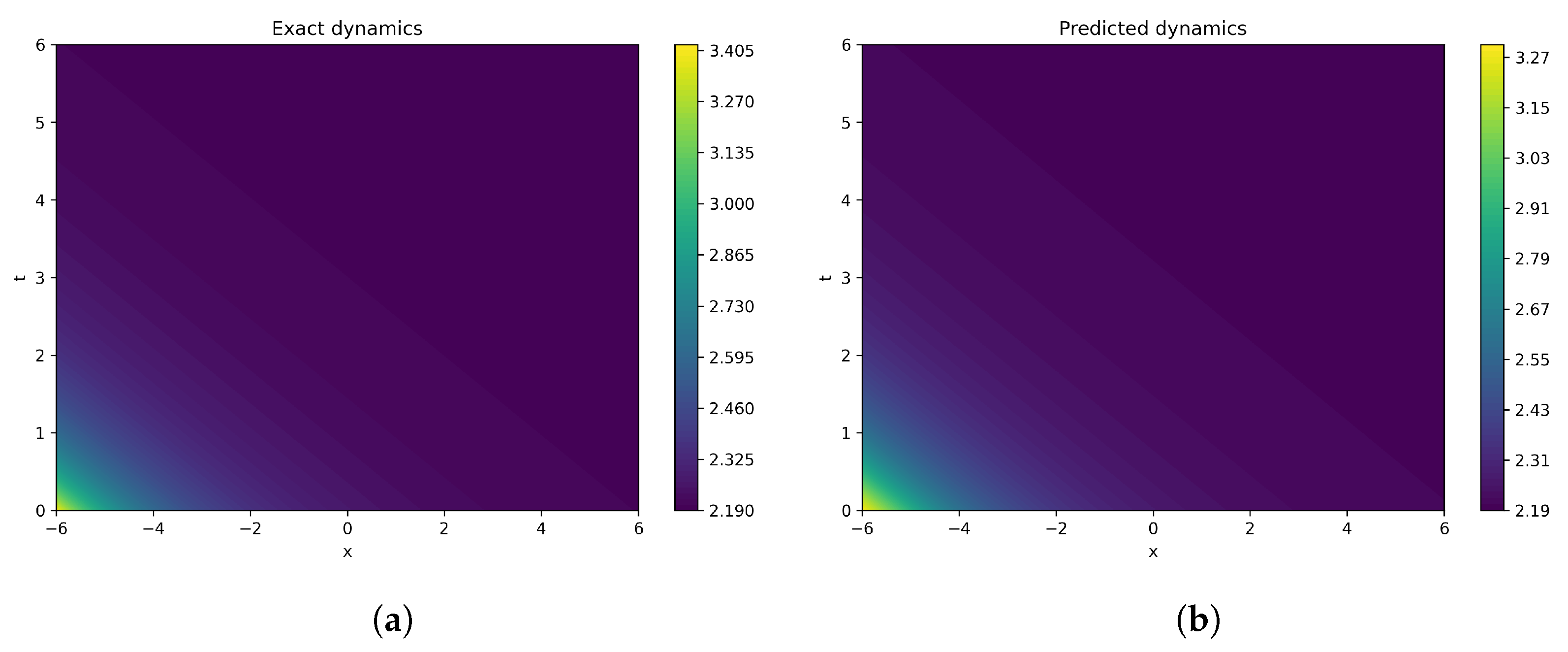
Moreover, the graph of the actual behaviour of solution (22) is presented in Figure 2 with different parametric values. Next, the MLP regressor neural network gives the almost similar to the actual data of the studied solution over 5000 epochs. Corresponding epoch-wise loss values, error tables, figures, and MSE loss values are provided below.

Furthermore, the actual and predicted behavior of solution (27) with the MLP regressor neural network is observed and discussed with the following corresponding epoch-wise loss values, error tables, figures, and MSE loss.

Moreover, over 5000 epochs, regarding the physical behaviour for solution (30), the actual and predicted data obtained through the application of the MLP regressor machine learning algorithm are approximately near to the results shown in Figure 4. Corresponding epoch-wise loss values, error tables, figures, and MSE loss values are provided below.

Furthermore, the dynamics of solution (31) with the actual and predicted behaviour over 10,000 epochs were observed and found to be similar to that in Figure 5, which was generated for solution (31). Corresponding epoch-wise loss values, error tables, figures, and MSE loss values are provided below.

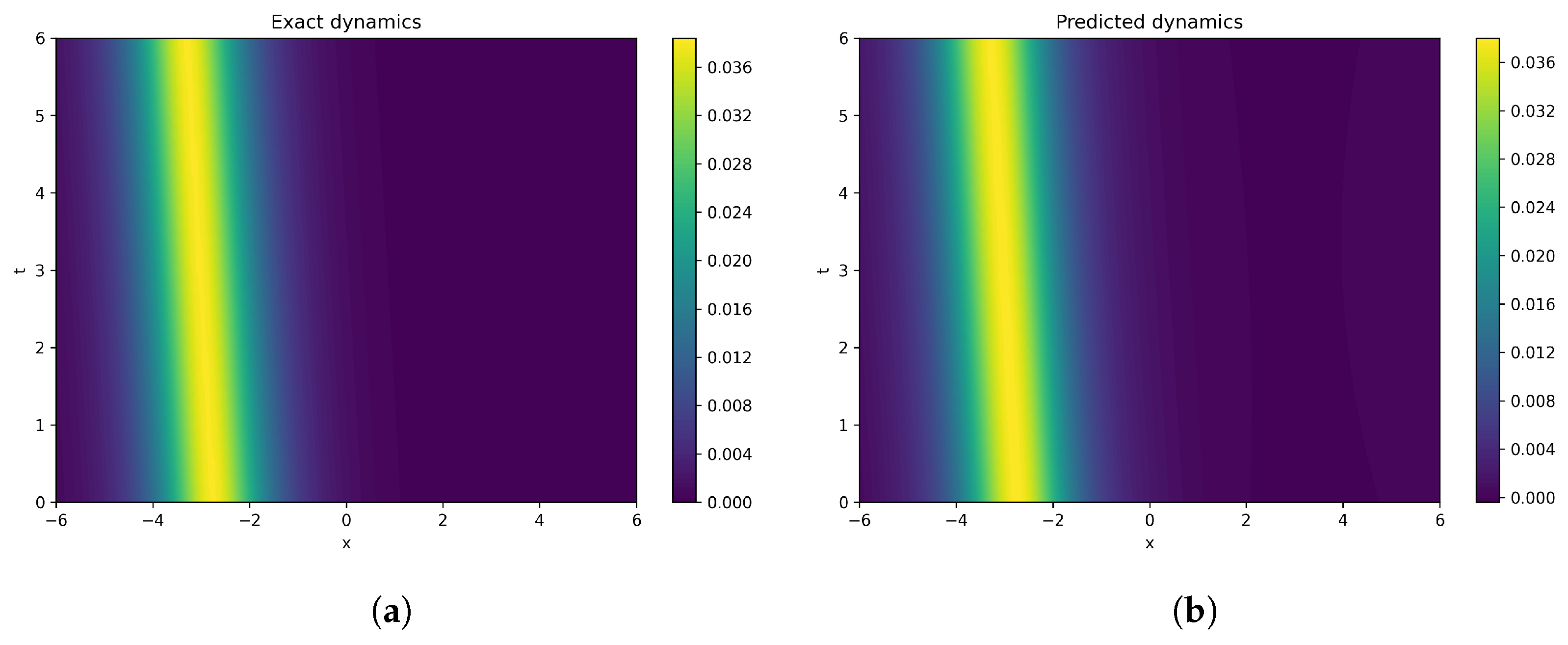
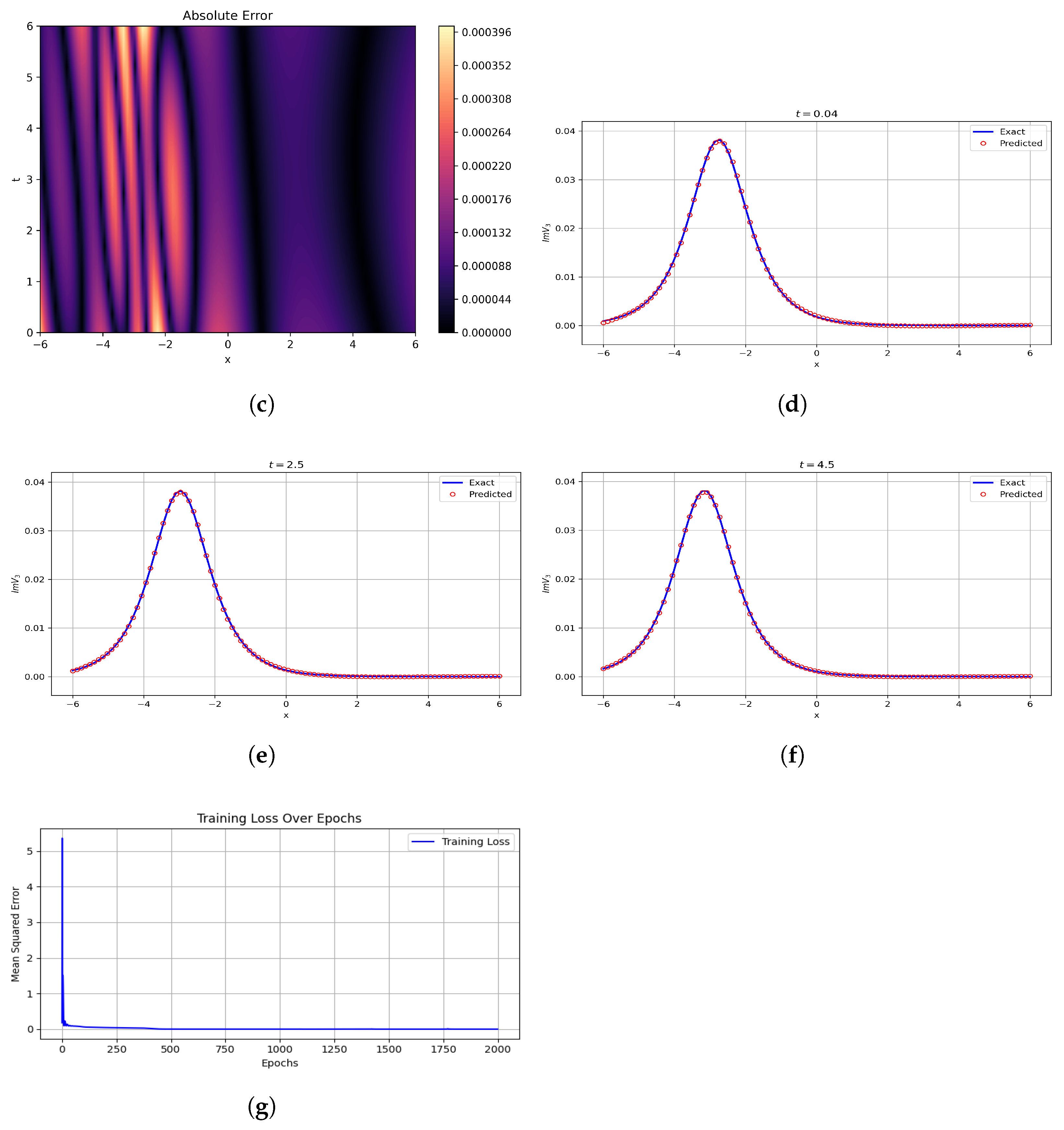
Moreover, regarding solution (36), its actual and predicted behaviour over 2000 epochs was observed, and it was found to be like in Figure 6. Corresponding epoch-wise loss values, error tables, figures, and MSE loss values are provided below.

Hence, the MLP regressor demonstrates strong robustness and high predictive accuracy, making it a highly effective machine learning model for simulating and forecasting the physical behaviors described by the given equations. Its ability to capture complex nonlinear relationships, generalize well to unseen data, and deliver reliable performance across various scenarios underscores its suitability for this application. Additionally, the model’s adaptability to different parameter configurations and computational efficiency further enhance its practical utility in data-driven physical modeling.

6. Chaotic Dynamics

To discuss the chaotic analysis, first through the application of the Galilean transformation, we define the perturbed system with an external periodic force for Equation (14) as

$$\left\{\begin{array}{c}{\displaystyle \frac{\mathrm{d}\Phi }{\mathrm{d}\xi }}=\phi ,\hfill \\ {\displaystyle \frac{\mathrm{d}\phi }{\mathrm{d}\xi }}={\displaystyle \frac{\phi }{a\beta \varrho }}+{\displaystyle \frac{({\alpha }^2-1)\Phi -{\Phi }^3}{a^2\alpha {\beta }^2\varrho }}+\gamma cos\left(\varpi \right),\hfill \\ {\displaystyle \frac{\mathrm{d}\varpi }{\mathrm{d}\xi }}=\chi ,\hfill \end{array}\right.$$

(46)

where $\varpi =\chi \xi$ and $\gamma$ and $\chi$ represent the strength and frequency of the external force. The sinusoidal forcing term $\gamma cos\left(\varpi \right)$ is employed as a generic, theoretically advantageous disturbance to examine the system’s robustness. In a physical Van der Waals context, such a term does not originate from internal thermodynamics but may signify an external, periodic effect. This could represent a mechanical vibration affecting the fluid container or a periodically driven pressure boundary. The relationship to the original, unperturbed system lies in its soliton solutions (kinks, bright/dark), which are the foundation of the analysis; the perturbation from the forcing affects these structures, indicating whether they endure or devolve into chaotic dynamics. This methodology is conventional for examining the structural stability of nonlinear waves, notwithstanding the idealized nature of the given force.

6.1. Return Map Technique

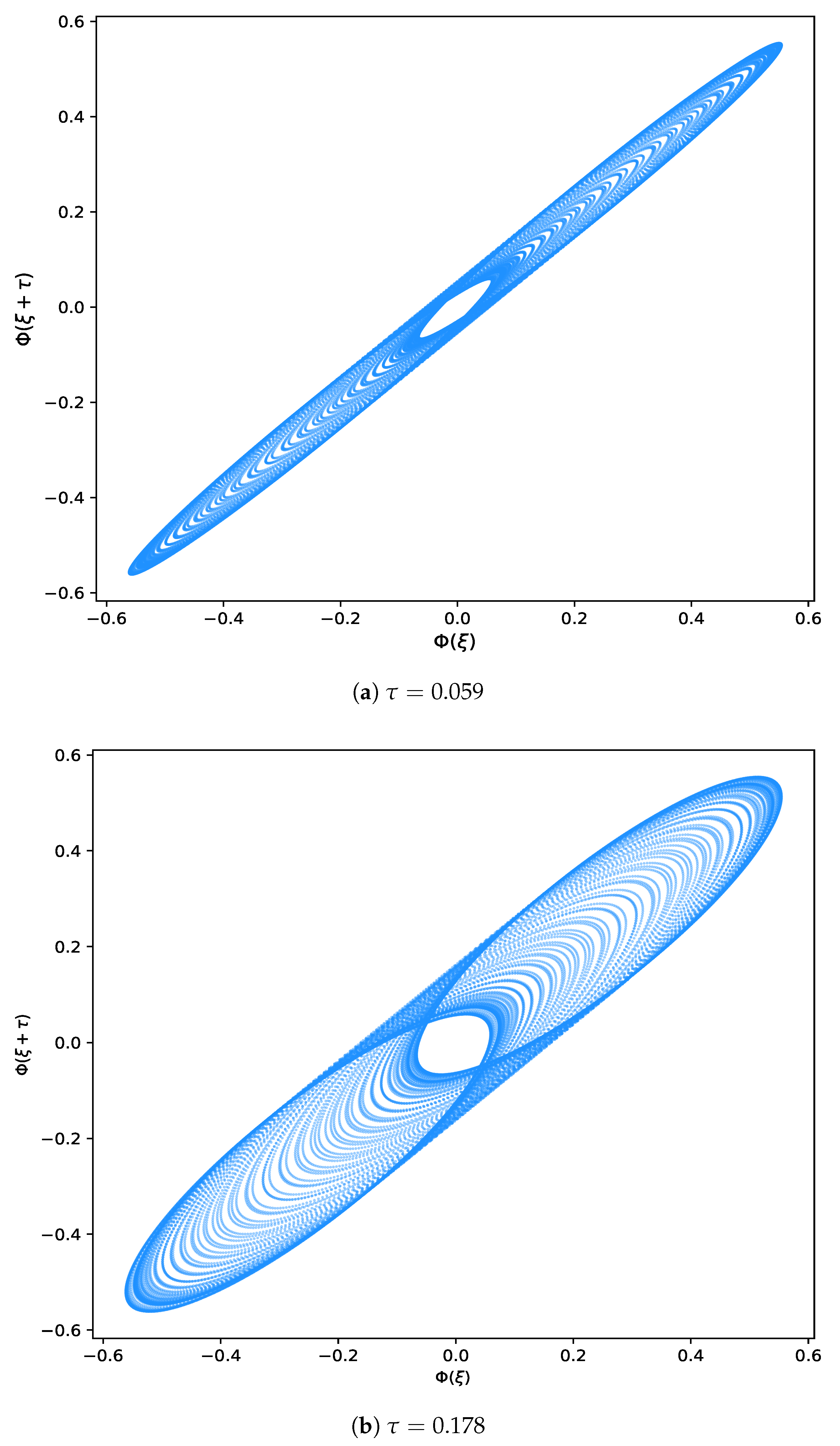
A return map simplifies a continuous system’s analysis by recording its state only at specific moments, when it crosses a Poincaré section. This discrete mapping is a powerful tool for detecting deterministic chaos, distinguishing it from random noise, and quantifying it through metrics like Lyapunov exponents. Its utility spans numerous fields, from analyzing neural activity and electronic oscillators to understanding turbulent fluids and vibrating mechanical systems. For the system described in Equation (46), Figure 7 and Figure 8 present the return map with $\Phi \left(\xi \right)$ on the horizontal axis and $\Phi (\xi +\tau )$ on the vertical axis, where $\tau$ represents the system’s characteristic decay time.

6.2. Bifurcation Diagram Technique

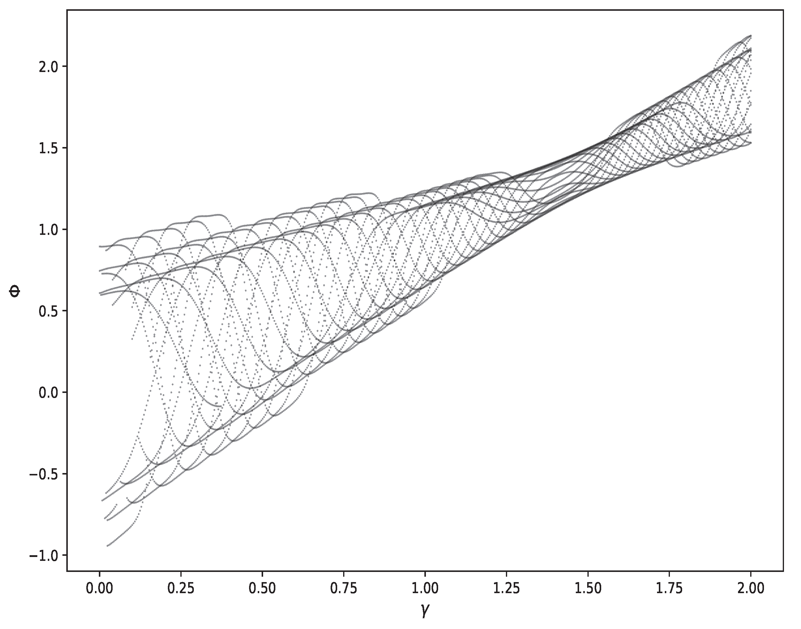
An effective tool for examining dynamic systems and comprehending chaotic behavior is a bifurcation diagram. It highlights transitions from orderly to chaotic states and graphically depicts how a system’s dynamics change as a key parameter changes. The diagram shows parameter values on the $\gamma$-axis and plots potential system states along the $\Phi$-axis. Complex structures, like branching patterns or sporadic intervals of stability, are frequently seen in chaotic regions. Figure 9 and Figure 10 illustrate the chaotic behavior for various parametric values.

6.3. Chaotic Attractor Technique

Chaotic attractor analysis is used to study chaotic systems in fields like meteorology, physics, and biology by visualizing complex, non-repeating trajectories in phase space. Its graphs reveal fractal structures and sensitivity to initial conditions, aiding in understanding turbulence, climate patterns, and neural activity. By plotting dynamic systems’ behavior over time, these attractors help identify stability, unpredictability, and hidden order within seemingly random data. Applications include weather forecasting, stock market analysis, and cardiac rhythm studies. The graphical representations provide insights into system dynamics, enabling better modeling and prediction of chaotic phenomena. Figure 11 was sketched to analyze the chaotic attractor’s behavior using parameters $a=0.011$, $\alpha =1.9$, $\beta =3.31$, $\varrho =0.1$, $\chi =0.04,4$, and $\gamma =5.023$ with different initial conditions.

6.4. Power Spectrum Technique

One essential tool for analyzing and characterizing dynamical systems is the power spectrum. It measures the distribution of a signal’s energy (or power) across various frequencies, exposing its underlying frequency structure and dominant periodicities. Researchers can detect chaos (through broadband noise-like spectra), identify important oscillatory modes, and differentiate between periodic, quasi-periodic, and stochastic behaviors in complex systems by looking at the power spectrum. The power spectrum of system (46) was analyzed for various parameters and initial conditions, as described in Figure 12, plotting log power against log frequency.

7. Conclusions

The dynamical aspects of the Van der Waals gas system were the focus of this study. The newly developed methodologies, including the F-expansion approach, mGREM, and generalized Arnous method were successfully applied to analyze the target model. Moreover, a variety of solitary wave solutions, such as dark, bright, and kink types, were combined, and periodic, hyperbolic, and exponential solutions were extracted. The extracted solutions are shown in Figure 1, Figure 2, Figure 3, Figure 4, Figure 5 and Figure 6 through the assistance of different parametric values. Solitary waves play a significant role in the Van der Waals gas model as they represent stable, localized disturbances with varying density or pressure that propagate without dissipation. These nonlinear waves arise due to the interplay between the gas’s non-ideal behavior (accounted for by Van der Waals corrections) and its thermodynamic properties, providing key insights into shock waves, phase transitions, and stability in dense gases. The graphs of these solitary waves, typically plotting pressure, density, or velocity against position, reveal their characteristic shape-preserving nature, helping researchers analyze how molecular interactions influence wave dynamics in real gases. Such studies are valuable in fields like fluid dynamics, condensed matter physics, and plasma physics, where understanding nonlinear wave behavior is essential for modeling complex systems. The MLP regressor effectively predicted the outcomes, yielding results that closely align with both our expected values and computational benchmarks, as shown in Figure 13, Figure 14, Figure 15, Figure 16, Figure 17 and Figure 18. Moreover, the training epochs as well as comparison of the exact and predicted dynamics of the solutions were discussed in the

Table 1. Training epochs and corresponding loss values for solution (19).

Epoch	100	200	300	400	500	600	700	800
Loss	0.170710	0.020170	0.003887	0.000609	0.000152	0.000076	0.000047	0.000032
Epoch	900	1000	1100	1200	1300	1400	1500
Loss	0.000022	0.000016	0.000012	0.000010	0.000008	0.000007	0.000006

,

Table 2. Comparison of exact and predicted dynamics with absolute error for solution (19).

x	t	Exact Dynamics	Predicted Dynamics	Abs Error
5.515152	6.000000	−0.987093	−1.004909	0.017816
−2.969697	0.000000	−1.297680	−1.314974	0.017293
−2.848485	0.000000	−1.168584	−1.185714	0.017130
5.636364	6.000000	−0.824881	−0.841860	0.016980
−2.848485	0.060606	−1.259463	−1.276432	0.016969
5.393939	5.939394	−1.036681	−1.053501	0.016820
5.515152	5.939394	−0.876396	−0.893108	0.016712
−2.727273	0.121212	−1.218925	−1.235237	0.016312
5.393939	5.878788	−0.927702	−0.943977	0.016275
5.393939	6.000000	−1.139471	−1.155319	0.015848

,

Table 3. Training epochs and corresponding loss values for solution (22).

Epoch	500	1000	1500	2000	2500
Loss	0.000745	0.000063	0.000031	0.000017	0.000009
Epoch	3000	3500	4000	4500	5000
Loss	0.000004	0.000002	0.000002	0.000001	0.000001

,

Table 4. Comparison of exact and predicted dynamics with absolute error for solution (22).

x	t	Exact Dynamics	Predicted Dynamics	Abs Error
−6.000000	0.000000	3.413469	3.290211	0.123258
−6.000000	0.060606	3.325903	3.247427	0.078476
−5.878788	0.000000	3.324144	3.246654	0.077490
−6.000000	0.121212	3.246589	3.201657	0.044933
−5.878788	0.060606	3.244993	3.200833	0.044160
−5.757576	0.000000	3.243400	3.200008	0.043391
−6.000000	0.181818	3.174495	3.153555	0.020940
−5.878788	0.121212	3.173041	3.152692	0.020349
−5.757576	0.060606	3.171591	3.151830	0.019761
−5.636364	0.000000	3.170143	3.150967	0.019176

,

Table 5. Training epochs and corresponding loss values for solution (27).

Epoch	500	1000	1500	2000	2500
Loss	0.000408	0.000049	0.000010	0.000005	0.000003
Epoch	3000	3500	4000	4500	5000
Loss	0.000002	0.000001	0.000001	0.000000	0.000000

,

Table 6. Comparison of exact and predicted dynamics with absolute error for solution (27).

x	t	Exact Dynamics	Predicted Dynamics	Abs Error
−0.303030	0.000000	0.820208	0.824301	0.004093
−0.303030	0.060606	0.818179	0.822127	0.003948
−0.060606	6.000000	0.259947	0.263823	0.003876
−0.303030	0.121212	0.816132	0.819935	0.003803
−0.424242	0.000000	0.893449	0.897245	0.003797
−0.060606	5.939394	0.262580	0.266285	0.003704
−0.424242	0.060606	0.892132	0.895835	0.003703
−0.181818	6.000000	0.391479	0.395139	0.003660
−0.303030	0.181818	0.814068	0.817726	0.003658
−0.424242	0.121212	0.890802	0.894411	0.003609

,

Table 7. Training epochs and corresponding loss values for solution (30).

Epoch	500	1000	1500	2000	2500
Loss	0.019716	0.019316	0.016621	0.002385	0.000108
Epoch	3000	3500	4000	4500	5000
Loss	0.000018	0.000011	0.000009	0.000007	0.000004

,

Table 8. Comparison of exact and predicted dynamics with absolute error for solution (30).

x	t	Exact Dynamics	Predicted Dynamics	Abs Error
−5.878788	3.636364	0.743171	0.756181	0.013010
−6.000000	3.696970	0.782161	0.795050	0.012889
−2.363636	1.393939	0.960486	0.947790	0.012696
−1.757576	1.030303	0.960167	0.947478	0.012689
−2.969697	1.757576	0.960801	0.948116	0.012685
−1.151515	0.666667	0.959844	0.947182	0.012662
−3.575758	2.121212	0.961112	0.948457	0.012655
−0.545455	0.303030	0.959517	0.946900	0.012617
−4.181818	2.484848	0.961418	0.948812	0.012606
−5.272727	3.272727	0.744183	0.756727	0.012544

,

Table 9. Training epochs and corresponding loss values for solution (31).

Epoch	1000	2000	3000	4000	5000
Loss	0.000039	0.000026	0.000030	0.000018	0.000007
Epoch	6000	7000	8000	9000	10000
Loss	0.000006	0.000005	0.000005	0.000006	0.000005

,

Table 10. Comparison of exact and predicted dynamics with absolute error for solution (31).

x	t	Exact Dynamics	Predicted Dynamics	Abs Error
−6.000000	0.000000	0.052329	0.062007	0.009678
−6.000000	0.060606	0.053142	0.062482	0.009340
−6.000000	0.121212	0.053967	0.062972	0.009004
−6.000000	0.181818	0.054806	0.063475	0.008669
−6.000000	0.242424	0.055657	0.063992	0.008335
−5.878788	0.000000	0.055650	0.063940	0.008290
−6.000000	0.303030	0.056521	0.064524	0.008003
−5.878788	0.060606	0.056514	0.064471	0.007958
−6.000000	0.363636	0.057399	0.065071	0.007672
−5.878788	0.121212	0.057391	0.065018	0.007627

,

Table 11. Training epochs and corresponding loss values for solution (36).

Epoch	200	400	600	800	1000
Loss	0.043448	0.021084	0.000336	0.000066	0.000023
Epoch	1200	1400	1600	1800	2000
Loss	0.000015	0.000011	0.000010	0.000009	0.000009

and

Table 12. Comparison of exact and predicted dynamics with absolute error for solution (36).

x	t	Exact Dynamics	Predicted Dynamics	Abs Error
−2.727273	6.000000	0.029166	0.029569	0.000402
−2.727273	5.939394	0.029306	0.029698	0.000392
−2.242424	0.000000	0.030559	0.030949	0.000390
−3.333333	6.000000	0.038128	0.037741	0.000387
−3.333333	5.939394	0.038111	0.037726	0.000386
0.060606	0.000000	0.001675	0.001874	0.000199
0.060606	0.060606	0.001662	0.001858	0.000196
0.060606	0.121212	0.001650	0.001843	0.000193
0.060606	0.181818	0.001638	0.001828	0.000190
0.060606	0.242424	0.001626	0.001813	0.000187

. The model demonstrated high accuracy, with predictions consistently approximating the target values within an acceptable margin of error. Its strong performance confirms the MLP regressor’s capability to reliably capture the underlying patterns in the data, making it a robust tool for predictive modeling in this context. For even greater precision, future refinements could include hyperparameter tuning, feature optimization, or ensemble techniques to further minimize deviations and enhance predictive consistency. Moreover, the inclusion of chaotic analysis, complemented by power spectra, return maps, chaotic attractors, and bifurcation diagrams, depicted the sensitive dependence on initial conditions and the complex structure of the system’s phase space. Figure 7, Figure 8, Figure 9, Figure 10, Figure 11 and Figure 12 were sketched for the visual representation of the chaotic techniques based on initial conditions and parametric values. These graphical tools collectively presented both qualitative and visual insights into the nonlinear dynamics and instabilities inherent in the studied model. The obtained solutions are relevant to several fields such as nonlinear dynamics, mathematical physics, engineering, and applied sciences. Researchers interested in the framework of nonlinear problems in applied sciences may find these findings interesting.

In addition, the generalized Arnous method, the modified F-expansion method, and the mGREM are all effective techniques for obtaining exact solutions of NLPDEs, each with its own strengths and limitations. The generalized Arnous method is flexible and capable of producing a wide range of solutions, including soliton and periodic forms, but it involves multiple arbitrary parameters, making validation more complex. The modified F-expansion method provides a systematic and straightforward way to generate hyperbolic, trigonometric, and periodic solutions, though it can become cumbersome for higher-order equations and may produce repetitive forms. The mGREM efficiently yields soliton, kink, and rational solutions by reducing the PDE to a solvable first-order ODE, but it is limited to equations compatible with the Riccati framework and can lead to complex algebraic systems. Overall, while all three methods produce rich solution families, they differ in formulation, complexity, and the types of solutions they most naturally generate. In future, the proposed methodologies can be employed to study various nonlinear dynamic behaviors of higher-dimensional systems with external effects, through stability analysis and the exploration of real-world applications.

References

1. Ecke, R.E. Chaos, patterns, coherent structures, and turbulence: Reflections on nonlinear science. Chaos Interdiscip. J. Nonlinear Sci. 2015, 25, 097605. [Google Scholar] [CrossRef]
2. Feigenbaum, M.J. Universal behavior in nonlinear systems. Phys. D Nonlinear Phenom. 1983, 7, 16–39. [Google Scholar] [CrossRef]
3. Nicolis, G. Introduction to Nonlinear Science; Cambridge University Press: Cambridge, UK, 1995. [Google Scholar]
4. Alonso, S.; Bär, M.; Echebarria, B. Nonlinear physics of electrical wave propagation in the heart: A review. Rep. Prog. Phys. 2016, 79, 096601. [Google Scholar] [CrossRef] [PubMed]
5. Ming, L.; Muhammad, J.; Yaro, D.; Younas, U. Exploring the multistability, sensitivity, and wave profiles to the fractional Sharma–Tasso–Olver equation in the mathematical physics. AIP Adv. 2025, 15, 045017. [Google Scholar] [CrossRef]
6. Roubíček, T. Nonlinear partial differential equations with applications; Springer Science & Business Media: Berlin/Heidelberg, Germany, 2013. [Google Scholar]
7. Ablowitz, M.J.; Clarkson, P.A. Solitons, Nonlinear Evolution Equations and Inverse Scattering; Cambridge University Press: Cambridge, UK, 1991. [Google Scholar]
8. Islam, M.E.; Khan, K.; Mannaf, M.A.; Akbar, M.A. Diffusion and degradation effect switching closed form solitons to a nonlinear mathematical model. Alex. Eng. J. 2025, 133, 272–283. [Google Scholar] [CrossRef]
9. Muhammad, J.; Bilal, M.; Rehman, S.U.; Nasreen, N.; Younas, U. Analyzing the decoupled nonlinear Schrödinger equation: Fractional optical wave patterns in the dual-core fibers. J. Opt. 2024, 1–12. [Google Scholar] [CrossRef]
10. Wadati, M. The modified Korteweg-de Vries equation. J. Phys. Soc. Jpn. 1973, 34, 1289–1296. [Google Scholar] [CrossRef]
11. Chen, X.; Yan, X.; Zhang, X.; Wang, F.; Suzuki, T.; Ohishi, Y.; Cheng, T. Highly sensitive nonlinear temperature sensor based on soliton self-frequency shift technique in a microstructured optical fiber. Sens. Actuators A Phys. 2022, 334, 113333. [Google Scholar] [CrossRef]
12. Zayed, E.M.; Alngar, M.E.; Shohib, R.; Biswas, A. Highly dispersive solitons in optical couplers with metamaterials having Kerr law of nonlinear refractive index. Ukr. J. Phys. Opt. 2024, 25, 01001-19. [Google Scholar] [CrossRef]
13. Arnous, A.H. Optical solitons with Biswas–Milovic equation in magneto-optic waveguide having Kudryashov’s law of refractive index. Optik 2021, 247, 167987. [Google Scholar] [CrossRef]
14. Butt, A.R.; Jhangeer, A.; Akgül, A.; Hassani, M.K. A plethora of novel solitary wave solutions related to Van der Waals equation: A comparative study. Sci. Rep. 2024, 14, 21665. [Google Scholar] [CrossRef]
15. Raza, N.; Rani, B.; Chahlaoui, Y.; Shah, N.A. A variety of new rogue wave patterns for three coupled nonlinear Maccari’s models in complex form. Nonlinear Dyn. 2023, 111, 18419–18437. [Google Scholar] [CrossRef]
16. Qiao, C.; Long, X.; Yang, L.; Zhu, Y.; Cai, W. Calculation of a Dynamical Substitute for the Real Earth–Moon System Based on Hamiltonian Analysis. Astrophys. J. 2025, 991, 46. [Google Scholar] [CrossRef]
17. Younas, U.; Muhammad, J.; Ali, Q.; Sediqmal, M.; Kedzia, K.; Jan, A.Z. On the study of solitary wave dynamics and interaction phenomena in the ultrasound imaging modelled by the fractional nonlinear system. Sci. Rep. 2024, 14, 26080. [Google Scholar] [CrossRef] [PubMed]
18. Duan, J.S.; Rach, R.; Baleanu, D.; Wazwaz, A.M. A review of the Adomian decomposition method and its applications to fractional differential equations. Commun. Fract. Calc. 2012, 3, 73–99. [Google Scholar]
19. Younas, U.; Muhammad, J.; Murad, M.A.; Almutairi, D.K.; Khan, A.; Abdeljawad, T. Investigating the truncated fractional telegraph equation in engineering: Solitary wave solutions, chaotic and sensitivity analysis. Results Eng. 2025, 25, 104489. [Google Scholar] [CrossRef]
20. Manas, M. Darboux transformations for the nonlinear Schrödinger equations. J. Phys. A Math. Gen. 1996, 29, 7721. [Google Scholar] [CrossRef]
21. Hosseini, K.; Samadani, F.; Kumar, D.; Faridi, M. New optical solitons of cubic-quartic nonlinear Schrödinger equation. Optik 2018, 157, 1101–1105. [Google Scholar] [CrossRef]
22. Muhammad, J.; Ali, Q.; Younas, U. On the analysis of optical pulses to the fractional extended nonlinear system with mechanism of third-order dispersion arising in fiber optics. Opt. Quantum Electron. 2024, 56, 1168. [Google Scholar] [CrossRef]
23. Bo, Y.; Tian, D.; Liu, X.; Jin, Y. Discrete Maximum Principle and Energy Stability of the Compact Difference Scheme for Two-Dimensional Allen-Cahn Equation. J. Funct. Spaces 2022, 2022, 8522231. [Google Scholar] [CrossRef]
24. Gu, Y.; Chen, B.; Ye, F.; Aminakbari, N. Soliton solutions of nonlinear Schrödinger equation with the variable coefficients under the influence of Woods–Saxon potential. Results Phys. 2022, 42, 105979. [Google Scholar] [CrossRef]
25. Hu, B.; Liao, Y. Convergence conditions for extreme solutions of an impulsive differential system. AIMS Math. 2025, 10, 10591–10604. [Google Scholar] [CrossRef]
26. Zhu, S.D. The generalizing Riccati equation mapping method in non-linear evolution equation: Application to (2 + 1)-dimensional Boiti–Leon–Pempinelle equation. Chaos Soliton Fractals 2008, 37, 1335–1342. [Google Scholar] [CrossRef]
27. Han, T.; Li, Z.; Li, C. Bifurcation analysis, stationary optical solitons and exact solutions for generalized nonlinear Schrödinger equation with nonlinear chromatic dispersion and quintuple power-law of refractive index in optical fibers. Physica A 2023, 615, 128599. [Google Scholar] [CrossRef]
28. Zhang, S.; Liu, L.; Wang, C.; Zhang, X.; Ma, R. Multistability and global attractivity for fractional-order spiking neural networks. Appl. Math. Comput. 2026, 508, 129617. [Google Scholar] [CrossRef]
29. Arnous, A.H. Optical solitons to the cubic quartic Bragg gratings with anti-cubic nonlinearity using new approach. Optik 2022, 251, 168356. [Google Scholar] [CrossRef]
30. Ozdemir, N.; Secer, A.; Ozisik, M.; Bayram, M. Optical soliton solutions of the nonlinear Schrödinger equation in the presence of chromatic dispersion with cubic-quintic-septic-nonicnonlinearities. Phys. Scr. 2023, 98, 115223. [Google Scholar] [CrossRef]
31. Kumar, S.; Hamid, I.; Abdou, M.A. Dynamic frameworks of optical soliton solutions and soliton-like formations to Schrödinger–Hirota equation with parabolic law non-linearity using a highly efficient approach. Opt. Quantum Electron. 2023, 55, 1261. [Google Scholar] [CrossRef]
32. Razzaq, W.; Zafar, A. Bilinearization of generalized Bogoyavlensky-Konopelchenko equation for Solitons with Neural Network: Painleve analysis. Nonlinear Dyn. 2025, 113, 25083–25096. [Google Scholar] [CrossRef]
33. Marchesin, D.; Plohr, B. Theory of three-phase flow applied to water-alternating-gas enhanced oil recovery, In Hyperbolic Problems: Theory, Numerics, Applications: Eighth International Conference in Magdeburg; Birkhäuser: Basel, Switzerland, 2001; pp. 693–702. [Google Scholar]
34. Fitt, A.D. Mixed systems of conservation laws in industrial mathematical modelling motion. Surv. Math. Ind. 1996, 6, 21–25. [Google Scholar]
35. Jhangeer, A.; Beenish. Dynamics and wave analysis in longitudinal motion of elastic bars or fluids. Ain Shams Eng. J. 2024, 15, 102907. [Google Scholar] [CrossRef]
36. Az-Zo’bi, E.A. Solitary and periodic exact solutions of the viscosity-capillarity Van der Waals gas equations. Appl. Appl. Math. Int. J. 2019, 14, 23. [Google Scholar]
37. Bilal, M.; Younis, M.; Rezazadeh, H.; Sulaiman, T.A.; Yusuf, A.; Rehman, S.U.; Younas, U. On the exact traveling wave solutions to the Van der Waals p-system. Int. J. Appl. Comput. Math. 2021, 7, 88. [Google Scholar] [CrossRef]
38. Arnous, A.H.; Mirzazadeh, M.; Hashemi, M.S.; Shah, N.A.; Chung, J.D. Three different integration schemes for finding soliton solutions in the (1 + 1)-dimensional Van der Waals gas system. Results Phys. 2023, 55, 107178. [Google Scholar] [CrossRef]
39. Jin, S. Numerical integrations of systems of conservation laws of mixed type. SIAM J. Appl. Math. 1995, 55, 1536–1551. [Google Scholar] [CrossRef]
Figure 1. Three dimensional (a), two dimensional (b) and density (c) plots of solution (19) for δ = 0.22 , A = 0.009 , β = 0.99 , ν 1 = 0.56 , and ρ = 2.89 .
Mathematics 13 03801 g001
Figure 2. Three dimensional (a), two dimensional (b) and density (c) plots of solution (22) for A = 0.23 , β = 9 , δ = 9.8 , ρ = 0.001 , and ϱ = 0.09 .
Mathematics 13 03801 g002
Figure 3. Three dimensional (a), two dimensional (b) and density (c) plots of solution (27) for a = 4.9 and ϱ = 0.01 .
Mathematics 13 03801 g003
Figure 4. Three dimensional (a), two dimensional (b) and density (c) plots of solution (30) for a = 4.1 and ϱ = 0.098 .
Mathematics 13 03801 g004
Figure 5. Three dimensional (a), two dimensional (b) and density (c) plots of solution (31) for a = 0.51 and ϱ = 0.089 .
Mathematics 13 03801 g005
Figure 6. Three dimensional (a), two dimensional (b) and density (c) plots of solution (36) for α = 0.09 , a = 1.6 , l 1 = 0.89 , l 0 = 0.02 , l 2 = 0.9 , and ν 1 = 0.09 .
Mathematics 13 03801 g006
Figure 7. Return map representation for system (46) for a = 0.15 , α = 0.9 , β = 0.31 , ϱ = 0.01 , χ = 2.9 , γ = 0.9 , and ( 0.31 , 0.47 , 0.89 ) .
Mathematics 13 03801 g007
Figure 8. Return map representation for system (46) for a = 0.15 , α = 0.9 , β = 0.31 , ϱ = 0.01 , χ = 2.9 , γ = 0.9 , and ( 0.31 , 0.47 , 0.89 ) .
Mathematics 13 03801 g008
Figure 9. Bifurcation diagram representation for system (46) for a = 0.5 , α = 0.35 , β = 0.64 , ϱ = 0.02 , χ = 1.9 , and ( 0.01 , 0.27 , 0.19 ) .
Mathematics 13 03801 g009
Figure 10. Bifurcation diagram representation for system (46) for a = 0.5 , α = 0.35 , β = 0.64 , ϱ = 0.02 , χ = 1.9 , and ( 0.21 , 0.42 , 0.8 ) .
Mathematics 13 03801 g010
Figure 11. Three-dimensional representation of the attractor of system (46) in phase space for a = 0.011 , α = 1.9 , β = 3.31 , ϱ = 0.1 , χ = 0.04 , and γ = 5.023 .
Mathematics 13 03801 g011
Figure 12. Power spectrum for system (46) for a = 0.1 , α = 0.23 , β = 1.31 , ϱ = 0.01 , χ = 0.5 , and γ = 5 .
Mathematics 13 03801 g012
Figure 13. (a,b) show the exact and predicted dynamics, with the absolute error in (c), while in (df), the blue line represents the actual data and the red circles show the predicted data behavior of solution (19). Moreover, the training loss with each epoch is represented in (g).
Mathematics 13 03801 g013aMathematics 13 03801 g013b
Figure 14. (a,b) show the exact and predicted dynamics with the absolute error in (c), while in (df), the blue line represents the actual data and the red circles show the predicted data behavior of solution (22). Moreover, the training loss with each epoch is represented in (g).
Mathematics 13 03801 g014aMathematics 13 03801 g014b
Figure 15. (a,b) show the exact and predicted dynamics with the absolute error in (c), while in (df), the blue line represents the actual data and the red circles show the predicted data behavior of solution (27). Moreover, the training loss with each epoch is represented in (g).
Mathematics 13 03801 g015aMathematics 13 03801 g015b
Figure 16. (a,b) show the exact and predicted dynamics with the absolute error in (c), while in (df), the blue line represents the actual data and the red circles show the predict data behavior of solution (30). Moreover, the training loss with each epoch is represented in (g).
Mathematics 13 03801 g016aMathematics 13 03801 g016b
Figure 17. (a,b) show the exact and predicted dynamics with the absolute error in (c), while in (df), the blue line represents the actual data and the red circles show the predicted data behavior of solution (31). Moreover, the training loss with each epoch is represented in (g).
Mathematics 13 03801 g017aMathematics 13 03801 g017b
Figure 18. (a,b) show the exact and predicted dynamics with the absolute error in (c), while in (df), the blue line represents the actual data and the red circles show the predict data behavior of solution (36). Moreover, the training loss with each epoch is represented in (g).
Mathematics 13 03801 g018aMathematics 13 03801 g018b