Abstract
This paper presents a new Residual-based Sparse Approximate Inverse algorithm, designed to be automatic, computationally efficient, and highly parallelizable. After briefly reviewing Frobenius-norm-based preconditioning techniques and identifying two key challenges in this class of methods, we introduce an improved approach that integrates adaptive strategies from the Power Sparse Approximate Inverse algorithm and incomplete LU factorization. The method leverages the Hamilton–Cayley theorem for effective sparsity pattern construction and employs LU decomposition for efficient implementation. Theoretical analysis establishes the convergence properties and computational features of the proposed algorithm. Numerical experiments using real-world data demonstrate that the proposed algorithm significantly outperforms established methods—including the Sparse Approximate Inverse, Power Sparse Approximate Inverse and Residual-based Sparse Approximate Inverse algorithms—with a Generalized Minimal Residual iterative solver, confirming its superior efficiency and practical applicability.
MSC:
65F10
1. Introduction
Most practical challenges encountered in industrial production and daily life can be formulated as problems within the realm of scientific computing. Among these, the solution to the following large sparse linear systems constitutes a core issue that our research focuses on:
where is a nonsymmetric coefficient matrix and is a given vector. The primary approaches for solving linear systems fall into two categories: direct methods and iterative methods. In most practical scenarios, the matrix A arises from the linearized discretization of partial differential equations, where the dimension n can be exceedingly large. Under such conditions, direct solution methods become infeasible due to excessive memory requirements and computational costs. Consequently, the use of iterative methods is often unavoidable [1,2,3,4,5,6,7,8].
Currently, the most widely used iterative methods can be broadly divided into two main categories. The first consists of stationary iterative methods based on matrix splitting. Among these, the most fundamental are the Jacobi, Gauss–Seidel, and Successive Over-Relaxation (SOR) iterations. More advanced variants include multigrid-like techniques, the Symmetric Successive Over-Relaxation (SSOR) iteration, Uzawa iteration, and the well-known Hermitian and Skew-Hermitian Splitting (HSS) iteration [9,10]—which have attracted significant scholarly attention—along with their various improvements and extensions. While these methods are straightforward in form and relatively easy to implement, their performance often depends critically on the choice of parameters; however, this dependency has been largely mitigated for the HSS method through effective preconditioning strategies. Notably, the work in [11] showed that, with a proper preconditioner, the parameter can be set to 1 optimally for a broad class of problems. The second major category comprises Krylov subspace methods. Among these, the most commonly applied are the Generalized Minimal Residual (GMRES) method [12], the Quasi-Minimal Residual (QMR) method [13], and the Biconjugate Gradient Stabilized (BICGSTAB) method [14]. However, Krylov iterative solvers often suffer from slow convergence when the coefficient matrix A exhibits unfavorable spectral properties or is ill-conditioned [10]. To accelerate their convergence, it is essential to incorporate preconditioning techniques designed to improve the conditioning of the system—ideally reducing the condition number of the matrix to close to one. At present, widely used preconditioning strategies encompass several major classes. These include general algebraic methods like incomplete LU (ILU) factorization and sparse approximate inverses. For structured problems, particularly those derived from partial differential equations, highly efficient alternatives are available, such as multigrid methods and structured preconditioners based on matrix algebras (e.g., [15,16,17,18]). The latter are defined by seeking an approximate inverse within a specific matrix algebra characterized by free parameters, rather than a prescribed sparsity pattern, offering a powerful compromise between accuracy and computational cost.
The rapid advancement of parallel computing highlights a fundamental principle: algorithms with high parallel efficiency are more likely to prevail in the future [19]. Fortunately, Krylov subspace-based iterative methods align well with this requirement, as key operations such as matrix–vector products, dot products, and vector updates can be efficiently parallelized in theory [6]. It should be acknowledged that conventional preconditioners, exemplified by ILU factorization, demonstrate excellent performance in iterative computation. Nevertheless, these methods often suffer from inherent limitations in parallelizability or require highly complex implementations to achieve parallel execution for specific problems [19,20].
The foundation of the most straightforward sparse approximate inverse approach rests on the assumption that a sparse matrix M can effectively approximate the inverse of the matrix A, denoted as [21]. This preconditioning matrix M is then employed either to reduce the condition number of the original system or to distribute the spectrum in a favourable way [22,23], thereby accelerating the convergence of iterative solvers for the linear equations. The core challenge involves constructing such a matrix M and efficiently solving the resulting right- or left-preconditioned system through iterative methods
It is evident that sparse approximate inverse preconditioners participate in the iterative solution process by constructing an explicit approximation M of . This implies that M operates via matrix–vector products throughout the computation, endowing the method with inherent parallelizability [5,24,25]. Moreover, in parallel computing environments, the overall performance of such preconditioners is highly dependent on the sparsity pattern and quality of M [6].
Another significant advantage of sparse approximate inverse preconditioners is their robustness [26]. Although incomplete factorization preconditioners often demonstrate strong performance, they are prone to various forms of numerical instability [27,28]. For example, even when applied to well-behaved symmetric positive definite matrices, standard incomplete Cholesky factorization may fail unless specific conditions are met—such as when the matrix is an H-matrix [29,30]. In contrast, sparse approximate inverse techniques are generally free from such limitations, contributing to their broader applicability [26].
Owing to the considerable advantages of sparse approximate inverse techniques [31], significant research attention has been attracted in recent years, supported by rigorous theoretical analyses that substantiate these benefits [5,25,32,33,34,35,36,37,38,39,40]. Currently, two main methodologies prevail for implementing sparse approximate inverse preconditioners: one relies on preprocessing through matrix factorization, while the other seeks preconditioners by minimizing the Frobenius norm, as in the case of the structurted preconditioning [15,16,18]. When matrix factorization is efficiently organized via an incomplete Gram–Schmidt procedure, the classic approximate inverse algorithm algorithm [33,34] emerges as a prominent representative of the first category. The second approach depends critically on two factors: predefined sparsity patterns and adaptive iterative algorithms, with the SParse Approximate Inverse (SPAI) algorithm [5] serving as the archetype in this class.
This paper introduces more effective algorithms designed to address specific challenges in the modeling of estuarine and coastal environments. Unlike the open ocean and continental shelf seas, these regions are characterized by complex shorelines, islands, and shoals, which introduce substantial dynamical and geometric complications. Practical limitations often hinder comprehensive empirical observation and data collection in such areas, making full reliance on measurements infeasible. Furthermore, since theoretical models are inherently simplified representations of reality, they alone cannot fully capture the complex physical processes occurring in coastal waters. In light of these constraints, numerical simulation becomes an essential tool for studying estuary and coastal dynamics.
Two primary types of numerical ocean models are widely used: those based on structured quadrilateral grids and those employing unstructured triangular grids. To achieve high resolution without prohibitive computational cost, we have developed an ocean model that utilizes two-way nested quadrilateral grids. By incorporating both hydrostatic and non-hydrostatic approximations, this model supports the simulation of multi-scale processes within a unified framework.
Following the model development, the emphasis shifts to its efficient numerical solution. The bidirectionally nested quadrilateral grid ocean model is specifically designed to capture the unique hydrodynamic features of estuaries and coastal zones, employing locally refined nested grids to enhance resolution. While this approach improves accuracy, it imposes stringent constraints on the time step and substantially increases computational cost. The resulting discretized linear systems are both large-scale and highly sparse [41,42]. Therefore, a key objective of this paper is to develop efficient parallel algorithms tailored to such systems, addressing the specific numerical challenges posed by this model.
We propose customized algorithms for the effective solution of these discretized linear equations. The coefficient matrices and right-hand side vectors used in our numerical experiments are derived from discretizations of the model at various resolutions. Specifically, four test cases are considered, with coefficient matrix dimensions of , , , and , respectively.
In this work, we introduce a new variant of the Residual-based Sparse Approximate Inverse (RSAI [43]) algorithm, designated the New RSAI (NRSAI) algorithm, which is designed to be automatic, computationally efficient, and highly parallelizable. Section 2 provides a concise overview of the original RSAI method, highlighting its ability to adaptively construct preconditioning matrices using residual-based information. In Section 3, we refine the RSAI approach by incorporating strategies inspired by the Power Sparse Approximate Inverse (PSAI [44]) algorithm and ILU factorization, tailoring it to the specific structure of our problem. These modifications improve the adaptive capabilities during iteration, leading to the proposed NRSAI algorithm. Section 4 presents its theoretical analysis, establishing its convergence properties and computational characteristics. Numerical experiments are conducted in Section 5 using real-world data to demonstrate the performance advantages of the NRSAI algorithm over the RSAI, SPAI, and PSAI algorithms. Finally, Section 6 summarizes the main contributions and findings of this study.
2. The RSAI Procedure
This section begins by presenting the conceptual foundation of our methodology, followed by a concise review of the Residual-based Sparse Approximate Inverse (RSAI [43]) algorithm.
The central objective of preconditioning is to construct a matrix M that serves as an efficient approximation to . This leads to the fundamental problem formulation:
where A is a known nonsingular coefficient matrix, M is the preconditioner to be solved, and E is the identity matrix.
Methods based on sparse approximate inverse preconditioners commonly reformulate this problem through Frobenius norm minimization:
over a space of matrices with a prescribed sparsity pattern, where is the Frobenius norm.
Owing to the separability and unitary invariance properties of the Frobenius norm, the global minimization problem decouples into n independent least-squares subproblems
with certain sparsity constraints on M, where is the k-th column of M and is the k-th column of E, .
This leads to the formulation of n independent least-squares problems that can be solved in parallel:
Let J denote the set of nonzero positions in , and define I as the set of row indices corresponding to nonzero rows in the submatrix . Due to the sparsity inherent in all components of (5), and by leveraging matrix-vector operation principles, the original large-scale least-squares problem is effectively reduced to a small-scale one:
This transformation substantially improves computational efficiency without compromising numerical accuracy. Further elaboration can be found in [5].
In general, determining an appropriate sparsity pattern for the preconditioner M of matrix A a priori is challenging without adequate structural information. Consequently, it is often necessary to adapt the sparsity structure of M dynamically during the iteration. Different algorithms employ distinct strategies to address this issue: the SPAI algorithm introduces an auxiliary least-squares problem; the PSAI algorithm adopts a theory-guided approach; whereas the RSAI algorithm utilizes residual information directly. The RSAI method is detailed as follows.
Consider, for instance, the solution process for the column vector , beginning with an initial sparsity pattern . Let and denote the sets of nonzero row and column indices, respectively, after l iterations. The problem solved at this stage can be expressed as:
and its complete residual
The residual corresponding to the local problem (7) is:
and it satisfies . If the convergence criterion is not met—i.e., —the current approximation is insufficient and requires refinement.
The RSAI algorithm leverages the residual itself to guide this process. Components of with larger magnitudes contribute more significantly to the residual norm. Therefore, prioritizing the reduction of these dominant entries accelerates convergence.
At each iteration, the algorithm examines the residual vector . Let contain the indices of all nonzero entries in . To avoid redundant updates, a set is maintained to track indices used in previous iterations. The entries of are sorted in descending order of absolute value, and the top entries not already in , are selected to form a new set . Then, update .
To reduce the residual components corresponding to , this set is used to identify new nonzero columns in , forming a column index set . If , the algorithm proceeds to the next iteration. Otherwise, the corresponding nonzero rows are identified, yielding a row index set . The index sets are updated as:
Further details on the solution procedure can be found in [43].
3. A New Residual-Based Sparse Approximate Inverse (NRSAI) Procedure
This section presents the proposed NRSAI algorithm (Algorithm 1) in detail.
| Algorithm 1 NRSAI |
|
We begin by describing the construction of the initial sparsity pattern for the sparse approximate inverse preconditioner M, adapted to the specific structure of the coefficient matrix A. As indicated in Section 2, the sparsity pattern J of each column vector significantly influences the resulting residual after solving the corresponding subproblem. A well-chosen pattern J that incorporates “high-quality” non-zero indices leads to a smaller -norm of the residual, thereby reducing the number of iterations required and improving overall computational efficiency. It is therefore essential to tailor the initial sparsity structure to the particular matrix A, rather than relying on generic templates.
Inspired by the PSAI algorithm, the sparsity pattern of M can be progressively refined using the Cayley–Hamilton theorem. According to [44], this theorem allows the inverse of A to be expressed as a matrix polynomial:
where denotes the identity matrix, and is a scalar coefficient for coming from those of the characteristic polynomial of A.
In essence, the non-zero pattern of the preconditioner M can be inferred from the union of non-zero patterns across various powers of the matrix A. For most non-singular sparse matrices, the sparsity structure of M generally differs from that of A. However, directly using high powers of A leads to prohibitive computational costs. Drawing inspiration from the extension from ILU(0) to ILU(1), and to balance computational expense with effectiveness, we construct the sparsity pattern for our preconditioner by taking the union of the inherently sparse non-zero patterns of the matrices E, A and . This approach allows us to capture more of the system’s connectivity while leveraging the naturally occurring sparsity of these operator matrices.
Since the columns of M are computed independently, we describe the procedure for a generic column . Based on the aforementioned strategy, an initial non-zero pattern for is constructed. The corresponding initial row index set is then defined as:
This allows the original problem to be reduced to an equivalent smaller-scale least-squares problem. Denoting , , and , the problem becomes:
Due to the moderate size and well-posed nature of this subproblem, it can be efficiently solved via LU decomposition in MATLAB. Once is obtained, the initial approximation to is constructed, and the full residual is computed as:
Moreover, if we define the reduced residual:
then it follows that .
We have established a well-defined initial problem and obtained its solution. The subsequent phase involves an adaptive iterative procedure, which focuses on the residual vector .
Under the initial configuration, let denote the current approximation produced by the NRSAI algorithm after a certain number of iterations, with corresponding row and column index sets I and J. Given a predefined tolerance , if , the current is considered acceptable; otherwise, further updates are performed iteratively until the residual condition is satisfied. To avoid introducing singularity in the preconditioner, the non-zero pattern of is gradually expanded during this process.
Similar to the RSAI algorithm, we extract key information from the individual entries of the residual. However, a fundamental distinction of our approach is that we consider not only the entries with the largest magnitudes, but also incorporate a dynamic threshold to identify multiple influential components.
The primary goal of the iteration is to reduce below . Thus, the residual itself guides the index selection. It is intuitively beneficial to prioritize reducing the components of with larger magnitudes, as they contribute more significantly to the norm. However, as the iteration progresses, the relative importance of these components may change. Therefore, we introduce an adaptive threshold parameter to systematically identify which residual entries are considered “large” at each step.
The iterative workflow of the NRSAI algorithm is as follows. Starting from the initial index sets and , suppose that after l iterations, the current approximation does not yet satisfy the tolerance condition. Denote the corresponding index sets as and , the residual as , and the set of already utilized indices as .
Given the identity
we may restrict our attention to the reduced residual vector . Its entries are sorted in descending order of absolute value. As in the RSAI algorithm, selected indices from are used to identify new column indices. To avoid redundant selections, previously chosen indices are excluded via the set , whose role is thus essential.
Define the candidate set
on which subsequent operations are performed.
In contrast to the RSAI method, we introduce a threshold parameter to guide the selection. An entry is considered significant only if its magnitude relative to the residual norm satisfies
If no such entry exists in a given iteration, the process terminates.
For example, suppose the indices corresponding to the c largest-magnitude entries in are . If , then no index is selected. If but , then the selected index set is .
Let denote the set of selected indices. Then, the new column indices are obtained as:
Correspondingly, the new row indices are given by:
The index sets are then updated as:
and the preconditioner column is refined by solving the enlarged least-squares problem:
Finally, the set of used indices is updated to .
Typically, the solution of problem (19) is achieved through QR decomposition. When leveraging the solution from the previous iteration, the computation can be accelerated using efficient updating techniques. For a comprehensive discussion, we refer the reader to [5,44]. Nevertheless, for certain structured matrices, problem (19) can be solved more effectively using LU decomposition within the MATLAB environment.
4. Theoretical Analysis
We now analyze the theoretical properties of the NRSAI algorithm described in the previous section.
As a method based on Frobenius-norm minimization, the columns of the preconditioner M in NRSAI are computed independently; thus, a direct guarantee of its nonsingularity is not available. Despite this, the general theory developed by Grote and Huckle [5], which connects the nonsingularity of M to the stopping tolerance and justifies its effectiveness—applies directly to our proposed algorithm.
Furthermore, according to [5], the sparsity pattern of the preconditioner M generated by the SPAI algorithm is bounded above. The analysis in [43] indicates that, due to the fundamental similarity in the iterative logic, the RSAI algorithm also produces a preconditioner M with bounded sparsity. This ensures that the sparsity constraint is maintained throughout the computation. Given the analogous iterative structure between the NRSAI and RSAI algorithms, the preconditioner M computed by the NRSAI algorithm is likewise sparse.
We now recall a result from [43] regarding the sparsity of M. Let denote the number of non-zero elements in a vector or matrix.
Theorem 1
([43]). Let be a preconditioner generated by the RSAI algorithm after iterations, and define for . For a specific column , let , , , , and . If the initial sparsity pattern is ,
Furthermore, there are
Similarly, we can discuss the relationship between the matrix M generated by the NRSAI algorithm and the various quantities in the algorithm.
Theorem 2.
Let be a preconditioner generated by the NRSAI algorithm after iterations, and define for . For a specific column , let , , and let c denote the maximum number of elements in the set across all iterations. If the initial sparsity pattern satisfies , then
Moreover, the total number of nonzero entries in M is bounded by
Proof.
For most sparse matrices requiring preconditioning, the initial sparsity pattern proposed in our method is non-empty and typically contains multiple elements. Although the size of this set influences computational efficiency and problem scale, it does not alter the underlying iterative process. Following a reasoning analogous to Theorem 1, we observe that each iteration adds at most non-zero entries to the sparsity pattern of . Hence,
while also , which together yield inequality (22). Combining (24) with the identity
we obtain the bound (23). □
5. Numerical Results
In this section we apply the proposed NRSAI algorithm to compute the preconditioner M for matrix A, which is then used within the preconditioned GMRES method [12]. Here, “IT” and “CPU” denote the arithmetic averages of the iteration counts and CPU times (in seconds) over 10 runs of the preconditioned GMRES solver, respectively. The ratio refers to the proportion of nonzeros between M and A. All numerical experiments in this section were conducted using MATLAB R2023a on a Dell R740 2U server equipped with dual Gold 6250 CPUs (16 cores, 32 threads per CPU, base frequency 3.9 GHz, maximum turbo frequency 4.5 GHz) and 128 GB of RAM.
The methodology for extracting the linear systems in this section begins with the spatial discretization of the underlying partial differential equations (governing estuarine and coastal dynamics) via finite differencing on unstructured quadrilateral grids. A critical aspect of the approach is the treatment of the two-way nesting interfaces, where high-order interpolation schemes are employed to couple solutions between grids of different resolutions. This entire discretization and grid-coupling process transforms the continuous problem into a large, sparse system of linear equations; see [45,46].
In the initial numerical tests, the dimension of the sparse linear systems is set to . Although this matrix size is relatively small from a practical standpoint, the underlying model remains consistent, allowing this lower-dimensional example to effectively validate the efficiency of the preconditioner constructed via the NRSAI algorithm; that is, we first validate the core functionality and robustness of the proposed preconditioner on a set of representative medium-scale problems (with ) under various conditions. This initial step is crucial for verifying the correctness and basic performance characteristics of our algorithm before progressing to large-scale tests that demonstrate its scalability.
Table 1 presents the numerical results of the NRSAI preconditioner combined with GMRES under different tolerance values and , respectively, with a maximum of 5 outer iterations. The results indicate that the NRSAI preconditioner significantly accelerates the convergence of GMRES in both iteration count and computation time compared to the unpreconditioned case. Moreover, variations in have negligible impact on the iteration count unless a very strict tolerance is used, while only slightly affecting the total runtime.
It is noteworthy that the purpose of this initial test (see Table 1 and Table 2) is to validate the core functionality and robustness of the proposed preconditioner. Therefore, we report the total CPU time to facilitate a clear, high-level comparison. A more detailed profiling of the computational cost, breaking down the time into preconditioner construction and GMRES solution, will be presented and discussed in the subsequent large-scale tests (see Table 3, Table 4 and Table 5).
Figure 1 illustrates the eigenvalue distributions of the original matrix A and the preconditioned matrix . Clearly, the preconditioner M effectively clusters the eigenvalues of A near 1.
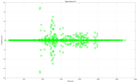
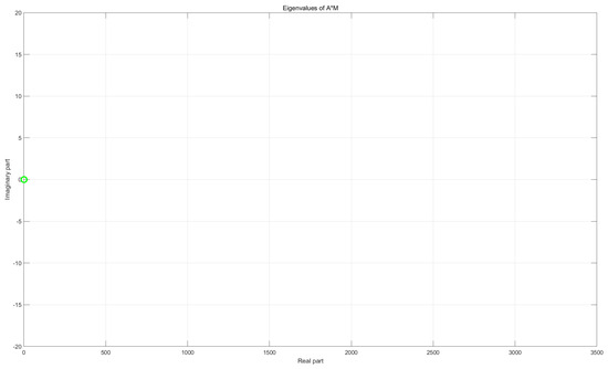
Figure 1.
Comparison of eigenvalue distributions before (top) and after (bottom) preconditioning, with problem dimension 2565× 2565.

Table 1.
Numerical results of GMRES under different for a 2565× 2565 system.
Table 1.
Numerical results of GMRES under different for a 2565× 2565 system.
| IT | CPU (Seconds) | |
|---|---|---|
| 28 | ||
| 12 | ||
| 12 | ||
| 12 | ||
| 12 | ||
| 9 |
Figure 2 further compares the eigenvalue distributions of for and under a magnified scale. The top and bottom subfigures correspond to and , respectively. It is evident that the eigenvalues are more tightly clustered when , which aligns with the superior performance observed in Table 1.
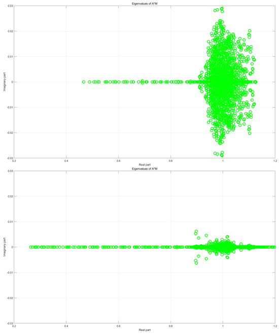
Figure 2.
Eigenvalue distributions of for (top) and (bottom). The problem dimension is 2565 × 2565.
For a quantitative assessment, Table 2 lists the values of under various norms, the spectral condition numbers of , and the density ratio for different . The results show that the values are very close for and , while a noticeable improvement occurs at , consistent with the earlier observations.
Table 2.
Quantitative measures under different , with problem dimension .
Table 2.
Quantitative measures under different , with problem dimension .
| Ratio | |||||
|---|---|---|---|---|---|
| 82422 | |||||
Finally, Figure 3 compares the sparsity patterns of the original matrix A, and the preconditioner M for and . It is clear that the sparsity pattern of effectively captures that of M.
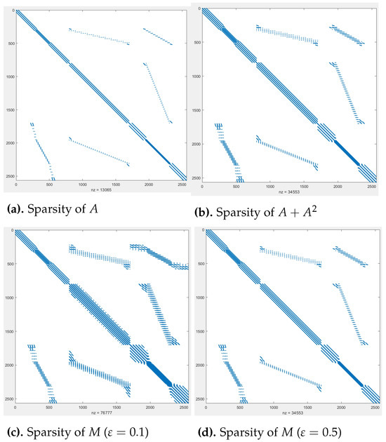
Figure 3.
Comparison of sparsity patterns, with problem dimension 2565 × 2565.
We further compare the NRSAI algorithm with other preconditioning methods. Here, denotes the time to construct the preconditioner, and are the solution time and iteration count of preconditioned GMRES, and . All results are averaged over 10 runs. GMRES is limited to 1000 iterations with a tolerance of .
Table 3 shows the results for a 15,601 × 15,601 matrix. The PSAI preconditioner leads to divergence, and SPAI increases total time despite reducing iterations. RSAI shows good speed in preconditioner construction and accelerates convergence effectively. The proposed NRSAI algorithm outperforms others, requiring only one-fourth of preconditioning time for the RSAI algorithm and achieving the shortest total solution time.
Table 3.
Results for a 15,601 × 15,601 matrix.
Table 3.
Results for a 15,601 × 15,601 matrix.
| Preconditioner | None | SPAI | PSAI | RSAI | NRSAI |
|---|---|---|---|---|---|
| 0 | 0.7094 | 0.0488 | 0.0157 | 0.0038 | |
| 0.3564 | 1.1469 | 86.4312 | 0.0137 | 0.0112 | |
| 0.3564 | 1.8563 | 86.4800 | 0.0294 | 0.0150 | |
| 42 | 10 | 1001 | 10 | 10 |
For a 20,785 × 20,785 matrix (Table 4), the PSAI algorithm again causes non-convergence, and the SPAI algorithm degrades further. The RSAI algorithm remains stable, while the NRSAI algorithm continues to excel in both preconditioning time and total solution time.
Table 4.
Results for a 20,785 × 20,785 matrix.
Table 4.
Results for a 20,785 × 20,785 matrix.
| Preconditioner | None | SPAI | PSAI | RSAI | NRSAI |
|---|---|---|---|---|---|
| 0 | 9.0689 | 0.0661 | 0.0753 | 0.0094 | |
| 1.4831 | 5.1409 | 137.3696 | 0.0926 | 0.0712 | |
| 1.4831 | 14.2098 | 137.4357 | 0.1679 | 0.0806 | |
| 109 | 24 | 1001 | 26 | 31 |
Finally, Table 5 presents results for the largest matrix, of size 34,737 × 34,737. Both PSAI and SPAI fail to yield effective preconditioning. The NRSAI algorithm consistently outperforms the RSAI algorithm in preconditioner construction time and solution efficiency.
Table 5.
Results for a 34,737 × 34,737 matrix.
Table 5.
Results for a 34,737 × 34,737 matrix.
| Preconditioner | None | SPAI | PSAI | RSAI | NRSAI |
|---|---|---|---|---|---|
| 0 | 4.4485 | 0.9641 | 0.2031 | 0.0617 | |
| 1.4286 | 7.4078 | 632.3594 | 0.1462 | 0.0426 | |
| 1.4286 | 11.8563 | 633.3235 | 0.3493 | 0.1043 | |
| 42 | 10 | 1001 | 10 | 10 |
6. Findings, Limitations, and Future Work
6.1. Key Findings
This work introduced the NRSAI preconditioner and demonstrated its efficacy through theoretical analysis and numerical experiments. The key findings are summarized as follows.
First, the proposed adaptive pattern selection strategy, underpinned by the Hamilton–Cayley theorem, was shown to be effective in capturing the essential non-zero structure of the inverse with low computational cost.
Second, the integration of techniques from the PSAI algorithm and ILU led to an algorithm that is both automatic and robust, eliminating the need for manual parameter tuning.
Third, extensive numerical tests on real-world problems confirmed that the NRSAI algorithm consistently outperforms established methods, including the SPAI, PSAI, and RSAI algorithms, in terms of iteration count and CPU time within a GMRES solver, underscoring its practical utility.
6.2. Limitations and Future Work
A limitation of the present numerical experiments is that they were conducted primarily on problems of a fixed dimension. A comprehensive analysis of the algorithm’s scalability and computational complexity across a wide range of problem sizes will be a central focus of our future work. Despite its promising performance, a limitation of the NRSAI algorithm is that the new algorithm only takes into account the specific characteristics of the rows and columns of the matrix during computation, without considering the overall structure of the matrix. Future work will focus on combining the overall structure with the specific structure of the rows and columns to propose a better algorithm.
7. Conclusions
This study opens with a concise overview of sparse approximate inverse preconditioning methods grounded in Frobenius norm minimization, outlining two central challenges common to such approaches.
Building on the PSAI algorithm, we emphasize the importance of the Hamilton–Cayley theorem in constructing effective sparsity patterns for the preconditioner. Motivated by techniques from incomplete LU factorization, a computationally efficient implementation of this theorem is developed, offering a solution to the first challenge.
Further examination of the RSAI algorithm reveals specific limitations, which are mitigated through an adaptive enhancement, thereby addressing the second challenge. By synergistically combining both solutions, we introduce a novel algorithm: NRSAI, an LU decomposition-based variant optimized for the class of problems considered in this work.
Numerical experiments were performed in two stages: initial tests confirmed the feasibility of the NRSAI algorithm, and subsequent comparative evaluations against the SPAI, PSAI, and RSAI algorithms within a GMRES framework demonstrated the significantly higher efficiency of the NRSAI algorithm.
Author Contributions
Conceptualization, X.-P.G. and R.-P.W.; methodology, J.-Q.T.; software, J.-Q.T.; validation, J.-Q.T., R.-P.W. and X.-P.G.; formal analysis, J.-Q.T. and X.-P.G.; investigation, J.-Q.T.; resources, X.-P.G., J.-Q.T. and R.-P.W.; data curation, J.-Q.T.; writing—original draft preparation, J.-Q.T. and X.-P.G.; writing—review and editing, X.-P.G., J.-Q.T. and R.-P.W.; visualization, X.-P.G. and R.-P.W.; supervision, X.-P.G. and R.-P.W.; project administration, R.-P.W. and X.-P.G.; funding acquisition, R.-P.W. and X.-P.G. All authors have read and agreed to the published version of the manuscript.
Funding
This work is partly supported by the National Key R&D Program of China (No. 2022YFA1004403), Science and Technology Commission of Shanghai Municipality (No. 22DZ2229014), National Natural Science Foundation of China (No. 12471377), the Opening Foundation of Shanxi Key Laboratory for Intelligent Optimization Computing and Blockchain Technology (No. IOCBT2024Z01).
Data Availability Statement
The data presented in this study are available on request from the corresponding author. Due to the terms of our collaboration agreement and the intellectual property rights retained by the originating institution, we are not authorized to publicly share this discretized dataset.
Acknowledgments
Warm thanks to the referees for their very pertinent and useful remarks. Also many thanks to Rui Ma for providing the matrices in the example, and thanks to Yu-Feng Hu for running some of the graphs in the example again.
Conflicts of Interest
The authors declare no conflicts of interest.
List of Abbreviations
| GMRES | Generalized Minimal RESidual algorithm |
| LU | LU factorization |
| ILU | Incomplete LU factorization |
| SPAI | SParse Approximate Inverse |
| PSAI | Power Sparse Approximate Inverse |
| RSAI | Residual-based Sparse Approximate Inverse |
| NRSAI | New Residual-based Sparse Approximate Inverse |
References
- Bacuta, C. A unified approach for Uzawa algorithms. SIAM J. Numer. Anal. 2006, 44, 2633–2649. [Google Scholar] [CrossRef]
- Bai, Z.-Z. Krylov subspace techniques for reduced-order modeling of large-scale dynamical systems. Appl. Numer. Math. 2002, 43, 9–44. [Google Scholar] [CrossRef]
- Barrett, R.; Berry, M.; Chan, T.; Demmel, J.; Donato, J.; Dongarra, J.; Eijkhout, V.; Romine, R.; Van Der Vorst, H.A. Templates for the Solution of Linear Systems; SIAM: Philadelphia, PA, USA, 1994. [Google Scholar]
- Benzi, M.; Haws, J.C.; Tůma, M. Preconditioning highly indefinite and nonsymmetric matrices. SIAM J. Sci. Comput. 2000, 22, 1333–1353. [Google Scholar] [CrossRef]
- Grote, M.J.; Huckle, T. Parallel preconditioning with sparse approximate inverses. SIAM J. Sci. Comput. 1997, 18, 838–853. [Google Scholar] [CrossRef]
- Janna, C.; Ferronato, M.; Gambolati, G. A block FSAI-ILU parallel preconditioner for symmetric positive definite linear systems. SIAM J. Sci. Comput. 2010, 32, 2468–2484. [Google Scholar] [CrossRef]
- Vasav, R.; Jourdan, T.; Adjanor, G.; Badahmane, A.; Creuze, J.; Athènes, M. Cluster dynamics simulations using stochastic algorithms with logarithmic complexity in number of reactions. J. Comput. Phys. 2025, 541, 114318. [Google Scholar] [CrossRef]
- Yazidi, Y.E.; Ellabib, A. An iterative method for optimal control of bilateral free boundaries problem. Math. Methods Appl. Sci. 2021, 44, 11664–11683. [Google Scholar] [CrossRef]
- Bai, Z.-Z.; Golub, G.H.; Ng, M.K. Hermitian and skew-Hermitian splitting methods for non-Hermitian positive definite linear systems. SIAM J. Matrix Anal. Appl. 2003, 24, 603–626. [Google Scholar] [CrossRef]
- Saad, Y. Iterative Methods for Sparse Linear Systems; SIAM: Philadelphia, PA, USA, 2003. [Google Scholar]
- Bertaccini, D.; Golub, G.H.; Capizzano, S.S.; Possio, C.T. Preconditioned HSS methods for the solution of non-Hermitian positive definite linear systems and applications to the discrete convection-diffusion equation. Numer. Math. 2005, 99, 441–484. [Google Scholar] [CrossRef]
- Saad, Y.; Schultz, M.H. GMRES: A generalized minimal residual algorithm for solving nonsymmetric linear systems. SIAM J. Sci. Stat. Comput. 1986, 7, 856–869. [Google Scholar] [CrossRef]
- Freund, R.W.; Nachtigal, N.M. QMR: A quasi-minimal residual method for non-Hermitian linear systems. Numer. Math. 1991, 60, 315–339. [Google Scholar] [CrossRef]
- Van Der Vorst, H.A. Bi-CGSTAB: A fast and smoothly converging variant of Bi-CG for the solution of non-symmetirc linear systems. SIAM J. Sci. Stat. Comput. 1992, 12, 631–644. [Google Scholar] [CrossRef]
- Benedetto, F.D.; Serra-Capizzano, S. Optimal multilevel matrix algebra operators. Linear Multilin. Algebra 2000, 48, 35–66. [Google Scholar] [CrossRef]
- Chan, T.F. An optimal circulant preconditioner for Toeplitz systems. SIAM J. Sci. Stat. Comput. 1988, 9, 766–771. [Google Scholar] [CrossRef]
- Chan, R.; Chan, T. Circulant preconditioners for elliptic problems. J. Numer. Linear Algebra Appl. 1992, 1, 77–101. [Google Scholar]
- Kailath, T.; Olshevsky, V. Toeplitz matrices: Structures, algorithms and applications. Calcolo 1996, 33, 191–208. [Google Scholar] [CrossRef]
- Ferronato, M.; Janna, C.; Pini, G. A generalized Block FSAI preconditioner for nonsymmetric linear systems. J. Comput. Appl. Math. 2014, 256, 230–241. [Google Scholar] [CrossRef]
- Benzi, M.; Tuma, M. A parallel solver for large-scale Markov chains. Appl. Numer. Math. 2002, 41, 135–153. [Google Scholar] [CrossRef]
- Janna, C.; Ferronato, M. Adaptive pattern research for block FSAI preconditioning. SIAM J. Sci. Comput. 2011, 33, 3357–3380. [Google Scholar] [CrossRef]
- Beckermann, B.; Kuijlaars, A.B.J. Superlinear convergence of conjugate gradients. SIAM J. Numer. Anal. 2001, 39, 300–329. [Google Scholar] [CrossRef]
- Beckermann, B.; Serra-Capizzano, S. On the asymptotic spectrum of finite element matrix sequences. SIAM J. Numer. Anal. 2007, 45, 746–769. [Google Scholar] [CrossRef]
- Barnard, S.T.; Bernardo, L.M.; Simon, H.D. An MPI implementation of the SPAI preconditioner on the T3E. Int. J. High Perform. Comput. Appl. 1999, 13, 107–123. [Google Scholar] [CrossRef]
- Chow, E.; Saad, Y. Approximate inverse preconditioners via sparse-sparse iterations. SIAM J. Sci. Comput. 1998, 19, 995–1023. [Google Scholar] [CrossRef]
- Benzi, M.; Cullum, J.K.; Tůma, M. Robust approximate inverse preconditioning for the conjugate gradient method. SIAM J. Sci. Comput. 2000, 22, 1318–1332. [Google Scholar] [CrossRef]
- Chow, E.; Saad, Y. Experimental study of ILU preconditioners for indefinite matrices. J. Comput. Appl. Math. 1997, 86, 387–414. [Google Scholar] [CrossRef]
- Elman, H.C. A stability analysis of incomplete LU factorizations. Math. Comp. 1986, 47, 191–217. [Google Scholar] [CrossRef]
- Manteuffel, T.A. An incomplete factorization technique for positive definite linear systems. Math. Comp. 1980, 34, 473–497. [Google Scholar] [CrossRef]
- Meijerink, J.A.; van der Vorst, H.A. An iterative solution method for linear systems of which the coefficient matrix is a symmetric M-matrix. Math. Comp. 1977, 31, 148–162. [Google Scholar] [CrossRef]
- Jia, Z.; Zhang, Q. Robust dropping criteria for F-norm minimization based sparse approximate inverse preconditioning. BIT Numer. Math. 2013, 53, 959–985. [Google Scholar] [CrossRef]
- Benzi, M.; Marín, J.; Tůma, M. A two-level parallel preconditioner based on sparse approximate inverses. In Iterative Methods in Scientific Computation IV; IMACS Series in Computational and Applied Mathematics, 5; Kincaid, D.R., Elster, A.C., Eds.; IMACS: New Brunswick, NJ, USA, 1999; pp. 167–178. [Google Scholar]
- Benzi, M.; Meyer, C.D.; Tuma, M. A sparse approximate inverse preconditioner for the conjugate gradient method. SIAM J. Sci. Comput. 1996, 17, 1135–1149. [Google Scholar] [CrossRef]
- Benzi, M.; Tuma, M. A sparse approximate inverse preconditioner for nonsymmetric linear systems. SIAM J. Sci. Comput. 1998, 19, 968–994. [Google Scholar] [CrossRef]
- Benzi, M.; Tuma, M. Numerical experiments with two approximate inverse preconditioners. BIT Numer. Math. 1998, 38, 234–241. [Google Scholar] [CrossRef]
- Benzi, M.; Tuma, M. A comparative study of sparse approximate inverse preconditioners. Appl. Numer. Math. 1999, 30, 305–340. [Google Scholar] [CrossRef]
- Bergamaschi, L.; Pini, G.; Sartoretto, F. Approximate inverse preconditioning in the parallel solution of sparse eigenproblems. Numer. Linear Algebra Appl. 2000, 7, 99–116. [Google Scholar] [CrossRef][Green Version]
- Chow, E. A priori sparsity patterns for parallel sparse approximate inverse preconditioners. SIAM J. Sci. Comput. 2000, 21, 1804–1822. [Google Scholar] [CrossRef]
- Field, M.R. An Efficient Parallel Preconditioner for the Conjugate Gradient Algorithm; Technical Report HDL-TR-97-175; Hitachi Dublin Laboratory: Dublin, Ireland, 1997. [Google Scholar]
- Gould, N.I.M.; Scott, J.A. Sparse approximate-inverse preconditioners using norm-minimization techniques. SIAM J. Sci. Comput. 1998, 19, 605–625. [Google Scholar] [CrossRef]
- Hackbusch, W. Iterative Solution of Large Sparse Systems of Equations; Springer: Cham, Switzerland, 2016. [Google Scholar]
- Trottenberg, U.; Oosterlee, C.W.; Schüller, A. Multigrid; Academic Press: San Diego, CA, USA, 2001. [Google Scholar]
- Jia, Z.; Kang, W. A residual based sparse approximate inverse preconditioning procedure for large sparse linear systems. Numer. Linear Algebra Appl. 2017, 24, e2080. [Google Scholar] [CrossRef]
- Jia, Z.; Zhu, B. A power sparse approximate inverse preconditioning procedure for large sparse linear systems. Numer. Linear Algebra Appl. 2009, 16, 259–299. [Google Scholar] [CrossRef]
- Ding, Z.; Zhu, J.; Chen, B.; Bao, D. A Two-Way Nesting Unstructured Quadrilateral Grid, Finite-Differencing, Estuarine and Coastal Ocean Model with High-Order Interpolation Schemes. J. Mar. Sci. Eng. 2021, 9, 335. [Google Scholar] [CrossRef]
- Ma, R.; Zhu, J.-R.; Qiu, C. A new scheme for two-way, nesting, quadrilateral grid in an estuarine model. Comput. Math. Appl. 2024, 172, 152–167. [Google Scholar] [CrossRef]
Disclaimer/Publisher’s Note: The statements, opinions and data contained in all publications are solely those of the individual author(s) and contributor(s) and not of MDPI and/or the editor(s). MDPI and/or the editor(s) disclaim responsibility for any injury to people or property resulting from any ideas, methods, instructions or products referred to in the content. |
© 2025 by the authors. Licensee MDPI, Basel, Switzerland. This article is an open access article distributed under the terms and conditions of the Creative Commons Attribution (CC BY) license (https://creativecommons.org/licenses/by/4.0/).