Article

An Online Learning Framework for Fault Diagnosis of Rolling Bearings Under Distribution Shifts

1
Institute of Sound and Vibration, Hefei University of Technology, Hefei 230009, China
2
Department of Biomedical Engineering, Hefei University of Technology, Hefei 230009, China
3
School of Electronic and Electrical Engineering, Bengbu University, Bengbu 233030, China
*
Author to whom correspondence should be addressed.
Mathematics 2025, 13(23), 3763; https://doi.org/10.3390/math13233763
Submission received: 14 August 2025 / Revised: 26 October 2025 / Accepted: 7 November 2025 / Published: 24 November 2025

Abstract

Fault diagnosis of rolling bearings is crucial for ensuring the maintenance and reliability of industrial equipment. Existing cross-domain diagnostic methods often struggle to maintain performance under evolving mechanical and environmental conditions. This limits their robustness in long-term real-world deployments. To address this, we propose a novel online learning framework that continuously adapts to distribution shifts using streaming vibration data. Specifically, the proposed framework consists of three core modules: the Feature Extraction Module that encodes raw vibration signals into low-dimensional latent representations; the Fault Sample Generation Module (comprising a generator and discriminator network) that synthesizes diverse fault samples conditioned on normal-condition data; and the Classification Module that incrementally adapts by leveraging both synthesized fault samples and streaming normal-condition signals. We also introduce a domain-shift indicator ScoreODS to dynamically control the transition between prediction and fine-tuning phases during deployment. Extensive experiments on both public and private datasets demonstrate that the proposed method outperforms the most competitive method, achieving about a 4% improvement in diagnostic accuracy and enhanced robustness for long-term fault diagnosis under distribution shifts.

1. Introduction

Rolling bearings are critical components in rotating machinery, and are widely used in industrial systems such as motors, turbines, and gearboxes. Their primary function is to reduce friction and support radial and axial loads. Due to harsh operating conditions, rolling bearings are vulnerable to a range of faults, including inner race faults, outer race faults, rolling element (ball or roller) defects, and cage defects [1,2,3]. Early and accurate fault diagnosis is critical for maintaining the operational safety and reliability of machinery.
In industrial scenarios, models are commonly trained in laboratory environments but deployed in complex and dynamic factory settings [4]. This exposes the model to unseen and changing operating conditions, where the test data distributions differ significantly from those encountered during training. This phenomenon is commonly referred to as the “domain shift”, which often leads to unexpected performance degradation [5]. Such domain shifts are frequently encountered in safety-critical systems like high-speed train traction units, where rolling bearings operate under variable speeds, heavy loads, and harsh vibration environments. The proposed study, conducted under a project on intelligent fault diagnosis for high-speed train components, aims to develop an adaptive diagnostic framework that remains reliable under these real-world operating conditions.
Existing studies in rolling bearings diagnosis tackle the domain shift problem primarily with Domain Adaptation (DA) [6,7,8,9], Domain Generalization (DG) [3,10,11,12], and Test-Time Adaptation (TTA) techniques [13,14]. DA methods aim to align the distributions between the source and target domains, leveraging unlabeled or partially labeled target domain data during training. DG approaches aim to learn domain-invariant representations from multiple source domains, enabling the model to generalize to unseen target domains without accessing any target data. TTA focuses on adapting the model during inference by utilizing the test data itself, often in an unsupervised or self-supervised manner, to mitigate distribution shifts at deployment time.
Despite their effectiveness, these methods typically assume that test samples are independent, which does not hold for time-correlated and non-stationary industrial vibration data. To address this limitation, online learning has emerged as a promising solution [15,16], enabling models to continuously adapt to streaming data during deployment. By incrementally adapting to distributional shifts in real time, online learning enables fault diagnosis systems to remain robust and responsive in dynamic, evolving industrial environments. Unlike conventional test-time adaptation methods that adjust model parameters only once using unlabeled test samples, the proposed framework performs continuous online learning, where the model is incrementally updated during operation based on streaming data and drift detection results. This enables long-term adaptation to evolving conditions rather than one-time calibration.
However, enabling online learning in such dynamic environments for fault diagnosis presents two significant challenges. (Challenge 1) The first is that online learning techniques typically require labeled or pseudo-labeled samples for model updating, while real-world bearing monitoring rarely provides labels. (Challenge 2) The second challenge lies in dynamically estimating distributional drift during online deployment and adaptively switching between inference and fine-tuning modes to improve generalization performance continuously. Addressing these challenges is crucial for ensuring robust and reliable online learning systems in industrial settings.
To address these challenges, we propose a novel online learning framework for rolling bearing fault diagnosis that continuously adapts to dynamic operating conditions by leveraging streaming data collected under normal operating states. The framework employs a generative–discriminative network to synthesize fault samples from normal-condition signals. In addition, an online domain-shift score is used to monitor distribution drift and determine when fine-tuning is needed during deployment. This framework enables stable adaptation without requiring real fault data. In summary, our study addresses an online learning scenario in rolling bearing diagnosis where the model is trained offline and incrementally adapted to evolving operating conditions, rather than being retrained on the full dataset. This setting is particularly practical for real-time industrial applications dealing with non-stationary data streams.
The main contributions of this paper are as follows:
  • We explore the novel online learning scenario for rolling bearing diagnosis, where the model is trained offline but adapted during deployment using only normal-condition data. Unlike traditional offline and cross-domain methods, this approach supports continuous updates, making it suitable for non-stationary data and real-time applications.
  • We propose a novel online learning framework that integrates generative–discriminative fault sample synthesis with a domain shift scoring mechanism, enabling the model to detect distributional drift in real-time and trigger adaptive fine-tuning without reliance on actual fault data.
  • Extensive experiments on public and private datasets of rolling bearings validate the effectiveness of our proposed online learning framework.

2. Related Works

2.1. Cross-Domain Fault Diagnosis in Rolling Bearings

Cross-domain fault diagnosis has emerged as a critical direction in intelligent fault detection for rolling bearings, primarily due to the difficulty of collecting sufficient labeled data under diverse working conditions [4]. Traditional machine learning methods often assume that training and testing data follow the same distribution, but this assumption rarely holds in practical scenarios involving varying loads, speeds, or working conditions [7,10,17]. To address this issue, several cross-domain paradigms have been proposed. Table 1 provides a summary comparison of these paradigms in terms of their assumptions, data availability, and typical applications in fault diagnosis.
  • Transfer Learning (TL) aims to transfer knowledge from a labeled source domain to a different but related target domain. In fault diagnosis, TL methods often fine-tune pretrained models from one operating condition to another [2,18,19,20,21,22].
  • Domain Adaptation (DA) focuses on reducing domain shifts between source and target domains, usually by learning domain-invariant features. This includes unsupervised DA methods that assume no labels in the target domain, which is especially practical in real-world fault scenarios [6,7,8,9].
  • Domain Generalization (DG) attempts to train models on multiple source domains so that they can generalize to unseen target domains without further adaptation. This paradigm is useful in fault diagnosis when deployment environments are unknown or change dynamically [3,10,11,12].
  • Test-Time Adaptation (TTA) adapts the model online using only a small amount of unlabeled target samples available during inference. Due to its practicality and efficiency, this paradigm is drawing increasing attention in real-world industrial applications [13,14].
  • Online Learning (OL) incrementally updates the model as new data arrives, enhancing robustness against distribution shifts over time [15,16]. Despite its potential advantages, the unsupervised scenario where only normal-condition data are available in dynamic environments remains underexplored, primarily due to the scarcity of labeled fault samples and the challenge of stable adaptation during deployment.
Specifically, Wang et al. [19] proposed a Subdomain Adaptation Transfer Learning Network (SATLN) to enhance cross-domain bearing fault diagnosis by jointly reducing marginal and conditional distribution shifts. The method introduces subdomain-level alignment and adaptive weighting across network layers, showing improved performance on multiple transfer tasks. The Deep Causal Factorization Network (DCFG) [3] is a domain generalization approach for cross-machine bearing fault diagnosis, which avoids the use of target domain data during training. It leverages causal inference to separate fault-relevant (causal) features from domain-specific (non-causal) ones, thereby enhancing generalization to unseen domains. Li et al. [14] proposed a novel test-time adaptation framework for cross-domain bearing fault diagnosis, aiming to adapt pretrained models during deployment using only mini-batch normal-condition test data. Their method transforms raw signals into informative embeddings, reduces noise via reconstruction loss, and decomposes features into domain-invariant fault components and domain-related healthy components. Xu et al. [16] proposed an online transfer CNN (OTCNN) for rolling bearing fault diagnosis, which transfers features from a pre-trained offline model to enable fast online adaptation. The method employs signal fusion and multi-core MMD to enhance accuracy while reducing training time.

2.2. Online Learning

Online learning has emerged as a promising paradigm for streaming data environments, particularly in scenarios with dynamic and non-stationary operating conditions. Unlike traditional offline models that require access to the entire dataset in advance, online learning methods update the model incrementally as new data arrive, enabling real-time adaptation to evolving system behavior. Online learning methods are commonly categorized into three types: supervised (with full-label feedback), limited feedback (with partial signals such as correctness), and unsupervised (no labels or feedback) [23]. In many fault diagnosis scenarios, models are deployed to new devices where only normal-condition data is available, without any fault labels or feedback. This setup falls under the category of online unsupervised learning.
In the domain of online unsupervised learning, several studies have explored methods that incrementally model normal system behavior and detect anomalies in streaming data. For example, Bhatia et al. [24] proposed MemStream, a memory-based online anomaly detection framework designed to handle streaming data under concept drift. Instead of continuously updating the autoencoder itself, it proposes a memory module to learn the dynamic trends in data without the need for labels. The memory module is updated incrementally to adapt to new trends while being robust to concept drift. Yang et al. [25] proposes an unsupervised method for online long-term voltage stability assessment using phasor measurement unit (PMU) data and a variational autoencoder (VAE). Unlike traditional methods that rely on physical models or hand-crafted features, the proposed VAE-based approach automatically extracts latent features that represent voltage and load levels, enabling real-time monitoring of voltage stability without labeled data or prior knowledge of system topology. Chua et al. [26] proposed as a low-power, unsupervised online learning algorithm for implantable seizure detection. After an initial offline training stage, SOUL performs continuous online updates directly on the device, enabling in situ adaptation to drifting EEG patterns without external supervision. Chen et al. [27] propose a camera-aware cluster-instance joint online learning (CCIOL) framework was proposed. It leverages online inter-camera K-reciprocal nearest neighbors (OICKRNs) to dynamically refine pseudo labels by generating soft cluster-level and multi-instance-level labels. Additionally, dual-level contrastive learning is used to correct noisy similarities and enhance feature discrimination during training. Alam et al. [28] developed a memristor-based neuromorphic system that enables unsupervised online learning and anomaly detection on edge devices, achieving high efficiency through analog in-memory computing without relying on cloud processing.
These works collectively demonstrate the effectiveness of unsupervised online learning across diverse tasks, particularly in situations where labeled data is unavailable. In this paper, we address an unexplored scenario in bearing fault diagnosis, involving only streaming data collected under normal operating conditions.

3. Methodology

In this section, we present the technical details of the proposed online learning framework for rolling bearing fault diagnosis, which uniquely adapts the diagnostic model using only normal-condition signals. Specifically, the proposed framework incorporates a WGAN-GP network [29] to generate synthetic data and model complex feature distributions under dynamic conditions. The framework also incorporates a drift-based scoring metric to detect whether newly arrived samples deviate significantly from the expected data distribution. This integration of drift assessment, anomaly scoring, and generative modeling constitutes the core novelty.
The framework is composed of three primary modules: (1) the Feature Extraction Module; (2) the Fault Sample Generation Module (G-Net & D-Net); and (3) the Classification Module. The overall architecture of the proposed framework is shown in Figure 1. The Feature Extraction Module processes the input signals and encodes them into compact, low-dimensional feature representations. At its core, the Fault Sample Generation Module (G-Net & D-Net) synthesizes fault samples for various fault conditions using only normal-condition signals, enabling the model to perform online learning and detect faults under domain shifts. The Classification Module continuously learns from both synthesized fault samples and real samples to adapt to changing operating conditions and accurately distinguish between normal and faulty states.
In the offline stage, the G-Net and D-Net learn to synthesize fault samples conditioned on real normal-condition samples, allowing the framework to simulate fault scenarios that are unavailable in real-world operations. Then, the Feature Extraction Module and the Classification Module are jointly trained using both real and generated signal samples.
In the online stage, the model operates in two phases: the prediction phase and the fine-tuning phase. To manage the transition between these phases, we design an indicator called the Score of Resistance on Online Domain Shift (ScoreODS), which determines when the model should switch from prediction to fine-tuning. This online learning process enables robust diagnostic inference based on continuously updated representations.
Furthermore, the proposed ScoreODS mechanism serves as a core component of an original online OOD-based learning framework. This framework includes: (i) online generation of simulated samples using a generative network; (ii) evaluation of whether these simulated samples correspond to fault conditions via ScoreODS; and (iii) detection of overall device distribution shifts.

3.1. Feature Extraction Module

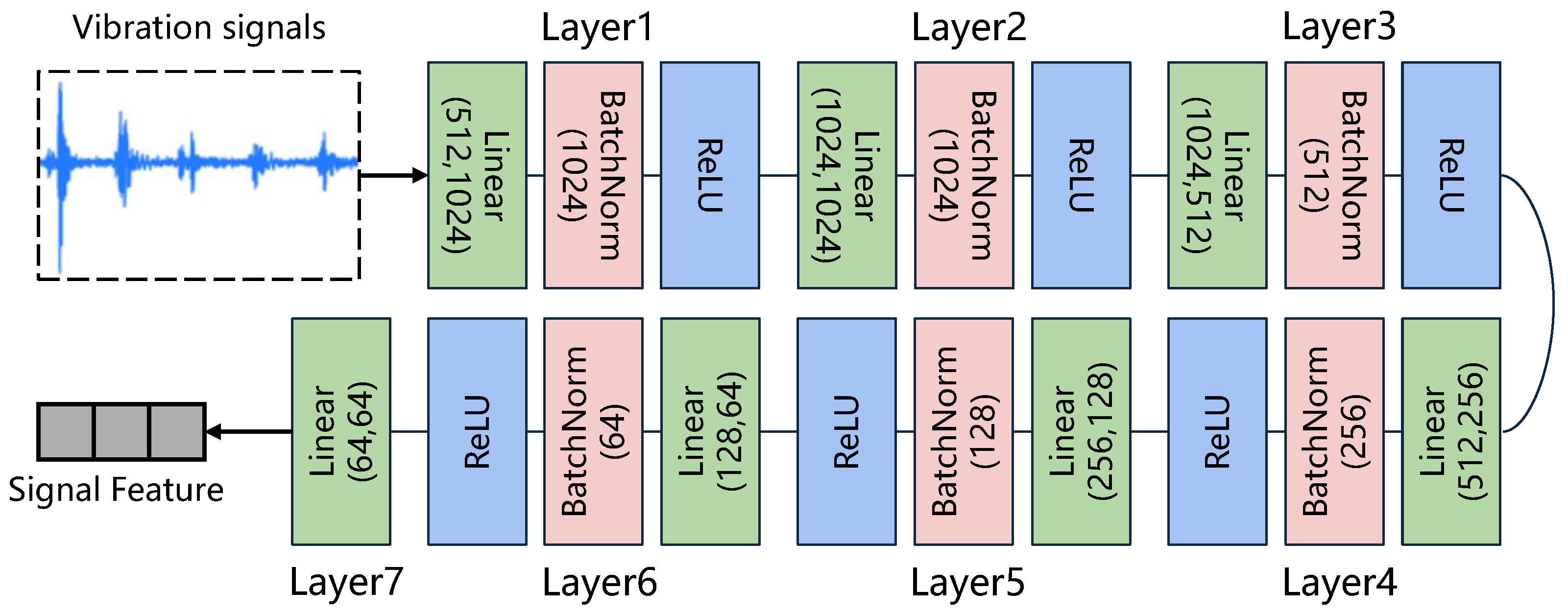
The Feature Extraction Module encodes input vibration signals x into low-dimensional feature representations in a latent space H . Without loss of generality, we utilize Multilayer Perceptron (MLP) as the Feature Extraction Module. As illustrated in Figure 2, the module consists of seven layers. In the first six layers, each layer is composed of a linear layer, a normalization layer, and an activation function, which can be formulated as follows:
h ( l ) = ReLU ( BN ( W ( l ) h ( l 1 ) + b ( l ) ) ) ,
where h ( l ) is the hidden representation of input signals in the layer l, and h ( 0 ) is the original input signal. W ( l ) and b ( l ) are the training weight matrix and the bias vector of the layer l.
The last (seventh) layer is a linear layer that maps the intermediate representation to the low-dimensional feature vector. Formally, the overall feature extraction process can be expressed as follows:
e = f FE ( x ) = W ( 7 ) h ( 6 ) + b ( 7 ) ,
where h ( 6 ) denotes the output of the sixth layer, e R d is the extracted feature vector, and d is its dimension.

3.2. Fault Sample Generation Module

In our online learning setting, a key challenge is the absence of labeled fault samples during deployment, since only normal-condition data are typically available in real-world industrial scenarios. To address this limitation, we design the Fault Sample Generation Module, which aims to synthesize fault samples from domain-shifted normal-condition signals. These generated samples serve as pseudo-fault data, enabling the model to adaptively learn without relying on actual fault labels.
In this work, generative models are employed within an online OOD detection framework to synthetically enrich the sample space and improve the robustness of drift detection. By learning the underlying data distribution, these models can simulate realistic samples and thereby augment scarce defect data, supporting more robust decision boundaries under dynamic or uncertain environments. Recent advances in generative modeling, such as VAE [30], Diffusion Models [31], and StyleGAN [32], have demonstrated remarkable capability in data synthesis and representation learning. However, these models are not well-suited for the objectives of this study. Specifically, the VAE relies on a reconstruction-based loss, which conflicts with our framework’s loss-driven drift evaluation. Diffusion Models, though powerful and stable, incur high computational costs that make them impractical for real-time or online detection. StyleGAN and other conditional generation architectures also struggle to maintain robustness under online out-of-distribution (OOD) detection scenarios. Consequently, WGAN-GP [29] achieves the most effective balance between generative expressiveness, training stability, and compatibility with our proposed online anomaly and drift detection framework.
We employ the Wasserstein Generative Adversarial Network with Gradient Penalty (WGAN-GP) [29] due to its improved training stability and ability to generate high-quality data samples. The network comprises two components: a generator (G-Net) and a discriminator (D-Net). A noise vector z N ( 0 , I ) , together with a normal-condition signal sample x s and an optional fault class label y , is fed into G-Net:
x ˜ = G ( x s , z , y ) , if multiple fault classes are considered , G ( x s , z ) , if only a single fault class exists ,
where x ˜ denotes the generated synthetic fault signal. G ( · ) represent the generator G-Net.
The generated sample x ˜ or real fault sample x f is then passed to D-Net, which outputs a scalar score indicating whether the input is real or generated:
D ( x ) R or D ( x , y ) R
where D ( x ˜ ) (or D ( x ˜ , y ) ) and D ( x f ) (or D ( x f , y ) ) denote the discriminator outputs for generated and real fault samples, respectively, in the absence or presence of class conditioning.
Notably, L G - Net is used to update only the generator parameters via backpropagation, whereas L D - Net is used to update only the discriminator parameters. The two networks are trained alternately to achieve adversarial learning. The D-Net loss is regarded as a critical metric for quantifying the discrepancy between the generated and real data. In what follows, we present the conditional formulation, as it generalizes to the single-class case by omitting the label y .
L D - Net = E x ˜ D ( x ˜ , y ) E x f D ( x f , y ) + λ E x ^ x ^ D ( x ^ , y ) 2 1 2
where x ˜ = G ( x s , z , y ) is the generated fault sample based on normal-condition sample x s , noise vector z , and fault class y . The third term is the gradient penalty enforcing the Lipschitz constraint [29], with λ as its coefficient. The interpolation samples x ^ are drawn uniformly along straight lines between x f and x ˜ .
The generator loss L G - Net combines the adversarial loss from WGAN-GP and a cross-entropy classification loss to ensure generated samples align with target fault categories:
L G - Net = E x ˜ , y D ( x ˜ , y ) σ E x ˜ , y log exp x ˜ T W g y c j = 1 C s exp x ˜ T W g y j
where x ˜ denotes the generated fault sample, y c is the one-hot encoded target class vector for that sample, W g is the learnable classification weight matrix, σ is the classification loss coefficient, and C s is the number of fault classes.
Finally, the generated fault samples x ˜ together with real samples x (including both normal-condition samples x s and fault samples x f ) are used to train the Feature Extraction Module and Classification Module. This approach helps to alleviate data imbalance and mitigate domain shift in feature representation.

3.3. Score of Resistance on Online Domain Shift

To monitor distributional drift of online data stream during deployment, we propose the Score of Resistance on Online Domain Shift (ScoreODS). This metric quantifies the deviation of the semantic representation of current normal-condition data from its baseline distribution established during offline training. We first compute the prototype (centroid) of the normal condition in the semantic space using the Feature Extractor module f FE :
c norm = 1 N s n = 1 N s f FE x s , n off
where x s , n off denotes the n-th normal-condition sample from the offline training set, and N s is the total number of offline normal samples.
During online monitoring, each incoming normal-condition sample x s is projected into the semantic space via f FE , and its Euclidean distance to the stored prototype c norm is calculated as follows:
d p = f FE ( x s ) c norm 2 , p = 1 , , N u
where N u denotes the number of online samples in the current monitoring window.
Similarly, for the offline baseline samples, the distance is defined as follows:
d q = f FE x s , q off c norm 2 , q = 1 , , N s .
The ScoreODS is then computed as the ratio of the average online distance to the average offline distance:
ScoreODS = 1 N u p = 1 N u d p 1 N s q = 1 N s d q .
The ScoreODS serves as an unsupervised indicator for online monitoring. A value close to 1 suggests that the distribution of current normal-condition data remains consistent with the baseline, whereas a higher value indicates potential distributional drift. This metric is intended solely for monitoring purposes and does not directly trigger model updates; however, persistent increases in ScoreODS may prompt manual inspection or adaptation in practical deployments.

3.4. Training Strategy

The proposed framework is trained in two stages: offline and online, each designed to address distinct operational requirements. The offline stage focuses on learning robust feature representations and synthesizing fault samples, while the online stage emphasizes adaptive updating under domain shifts using only normal-condition data.

3.4.1. Offline Stage

Labeled normal and fault samples are available during offline training. The training proceeds in two stages:
(1) The Fault Sample Generation Module (G-Net and D-Net) is first trained using the losses of L D - Net and L G - Net , with alternating updates to achieve stable and realistic fault sample synthesis. The Fault Sample Generation Module, consisting of the generator G and discriminator D, is trained in an adversarial manner by solving the following weighted minimax optimization problem:
min G max D α L D - Net + β L G - Net
where α and β are weighting coefficients balancing the discriminator and generator losses.
(2) Once the generator and discriminator have been trained, the Feature Extraction and Classification Modules are trained using the diagnosis loss L CE , which is the standard cross-entropy loss applied to both real and synthesized samples for classification.

3.4.2. Online Stage

During deployment, only normal-condition samples are observed. The online phase consists of: (1) Prediction Phase, where incoming samples are processed by the Feature Extraction Module and monitored via ScoreODS. The Fault Sample Generation Module synthesizes fault samples from normal-condition data to cover possible fault classes. These generated fault samples are then randomly mixed with the normal-condition samples for online learning. (2) Fine-tuning Phase, triggered by persistent domain shift, where the Classification Module is fine-tuned on a combined set of real normal samples and stored synthetic faults, while the Feature Extraction Module is frozen and the Fault Sample Generation Module is deactivated.

4. Experiments

To validate the effectiveness of our proposed framework, we conduct experiments on three datasets, including two public datasets and one private dataset, on rolling bearing diagnosis. In this section, we report our experimental settings and results in detail.

4.1. Datasets

We conduct experiments on three datasets. Notably, our dynamic cross-domain adaptation experiments are centered on three prevalent fault categories: normal condition (NC), inner race failure (IF), and outer race failure (OF).
  • Dataset A: The first dataset is the widely recognized Case Western Reserve University (CWRU (https://engineering.case.edu/bearingdatacenter, accessed on 1 March 2025)) bearing collection, which is a widely used benchmark for bearing fault diagnosis. This dataset contains both normal and faulty samples. The faults are classified according to the fault location (inner race, outer race, and rolling element) and fault severity, typically at diameters of 0.007, 0.014, and 0.021 inches. This dataset contains vibration signals captured by accelerometers from a test stand operating under motor loads ranging from 0 to 3 horsepower and speeds between 1720 and 1797 RPM. For this study, we utilized signals from the drive-end bearings, which were recorded at a sampling rate of 12 kHz. A total of 1200 samples were extracted for each of the specified fault conditions.
  • Dataset B: Our second source is the Mechanical Failures Prevention Group (MFPT (https://www.kaggle.com/datasets/emperorpein/mfpt-fault-datasets, accessed on 1 March 2025)) Society’s bearing dataset. It provides data from bearing test rigs, including baseline (normal) operations as well as conditions with inner and outer race faults under varying loads. A notable characteristic is the difference in acquisition parameters: normal condition data was gathered at 97,656 Hz under a 270 lbs load, while fault data was recorded at 48,828 Hz across three separate loads (200 lbs, 250 lbs, and 300 lbs). To ensure uniformity, all vibration signals were standardized by resampling them to 12 kHz. From this processed data, 600 samples were generated for each fault type.
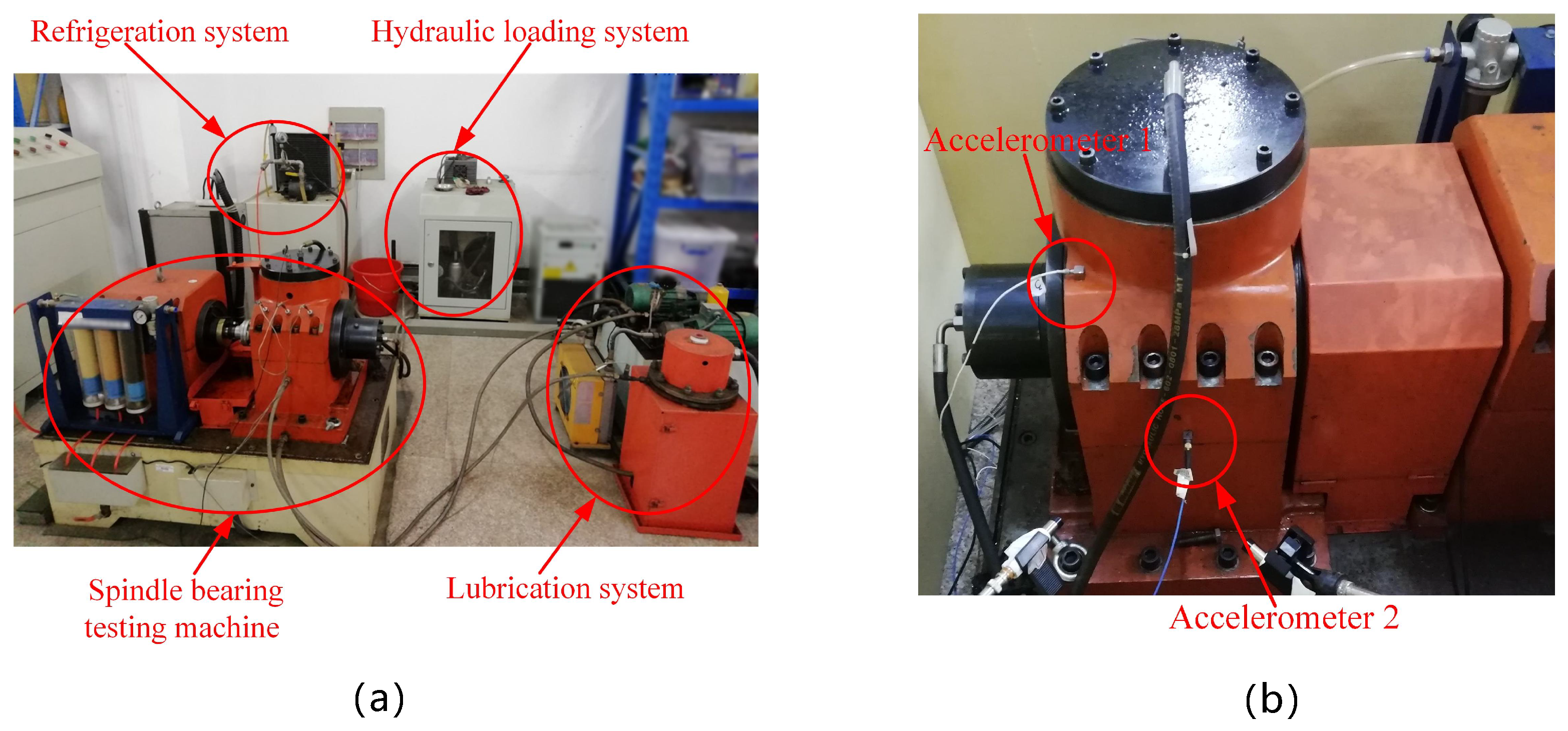
  • Dataset C: The third dataset is a private collection from the Hefei University of Technology in China. The data originates from a laboratory-based aero-engine bearing test rig (depicted in Figure 3), which integrates a spindle testing machine with hydraulic loading, lubrication, and refrigeration systems. The components under examination were NSK’s single-row cylindrical roller bearings, specifically models NU1010EM and N1010EM. Artificial damage was induced on healthy bearings using laser marking and wire cutting to create single- and multi-point failures, each measuring 9 mm in length by 0.2 mm in width. All experimental data was acquired with a 2 kN axial load, a motor speed of 2000 rpm, and a sampling frequency of 20.48 kHz. For each class of bearing condition, 2000 individual samples were compiled for the experiments.
It is worth noting that we do not present the results for the independent and identically distributed (IID) setting because the performance of all models, including our own, is saturated as shown in [14], which offers little comparative insight.
Datasets are partitioned into training, validation, and test subsets at an 8:1:1 ratio. To mitigate overfitting and determine the final performance, training ceases after five consecutive epochs with no improvement in validation loss, followed by a subsequent evaluation on the test sets. For test-time adaptation and online learning assessments, models are exclusively trained and validated using source domain data before evaluation on target domains.
The format of input data and the normalization strategy have a critical impact on model performance. In this study, we employ frequency-domain representations of the raw signals as the input type for all benchmarked approaches. Normalization refers to signal-level scaling of the input data to the range of [−1, 1], which serves as a standard preprocessing step to stabilize training and ensure consistent input scale, whereas the resampling process is only used to align signal segments in time and does not modify their intrinsic statistical properties, thus having negligible influence on diagnostic accuracy.

4.2. Comparison Methods

Our approach is benchmarked against diverse methods categorized into three architectural families: autoencoders, convolutional neural networks (CNNs), and recurrent neural networks (RNNs).
  • Autoencoder (AE) [33]: First proposed in [34], this architecture jointly learns an encoder and decoder to reconstruct original inputs from low-dimensional embeddings.
  • Denoising AE (DAE) [35]: Enhances representation robustness by reconstructing clean inputs from corrupted versions (Gaussian noise/dropout erasures), functioning as a regularizer for error correction.
  • Sparse AE (SAE) [36]: Addresses bias-variance tradeoffs through sparsity constraints (e.g., KL divergence) applied to hidden representations, trained via decoder-output/input distance minimization.
  • Symmetric Wasserstein AE (SWAE) [37]: Aligns data and latent distributions symmetrically while combining reconstruction loss for representation balancing.
  • AlexNet [38]: This pioneering CNN (2012) revolutionized image classification via convolutional layers, ReLU activations, and GPU acceleration, establishing foundational computer vision benchmarks.
  • ResNet-18 [39]: Solves gradient dissipation in deep networks via residual connections, enabling ultra-deep architectures. The 18-layer variant serves as our baseline.
  • BiLSTM [40]: Processes sequences bidirectionally using forward/backward LSTMs to capture contextual dependencies in time-series and language applications.
  • c-GCN-MAL [41]: A deep clustering architecture combining graph convolutional networks with adversarial learning for cross-domain fault diagnosis, enhancing transfer capabilities.
  • DCFN [3]: Deep causal factorization network that isolates cross-machine generalizable fault representations (causal factors) from domain-specific features (non-causal factors) using structural causal models. Evaluated using single training datasets treated as multi-source domains.
  • TTAD [14]: A test-time adaptation framework for cross-domain rolling bearing fault diagnosis, which adapts pre-trained models using limited target-domain normal-condition data. It transforms signals into embeddings, decomposes them into domain-related healthy and domain-invariant faulty components, and re-identifies target normal signals.

4.3. Implementation Details

To ensure fair comparison, we maintain identical hidden dimensions across all input signal encoders. Other baseline network parameters adhere to their original publications for optimal performance, with unified input/output layer dimensions fixed at 64. All baselines employ identical classifier architectures.
Model parameters are initialized using the Xavier method [42] and optimized via AdamW. Training employs a 0.001 initial learning rate, 2 regularization coefficient of 10 4 , batch size of 64, and 100-epoch duration. To facilitate later online learning stage requiring reduced learning rates, we implement an exponential decay schedule:
η ( t ) = η ( t 1 ) · γ t
All datasets undergo 8:1:1 splits for training, validation, and testing. Hyperparameters, except those specified above, are tuned via a validation set grid search. Bearing faults are standardized to three classes: normal condition (NC), inner race failure (IF), and outer race failure (OF). The evaluation protocol involves: 1. Training models on a source domain (e.g., Dataset A). 2. Online stage using limited NC samples 1, 5, 10, 50, 100 from the target domain (e.g., Dataset B). 3. Evaluating diagnosis accuracy and F1-scores on the full target domain.

4.4. Performance Comparison Under Cross-Domain Setting

As shown in Table 2, under the cross-domain setting, conventional autoencoder-based methods (AE, DAE, SAE, SWAE) exhibit low diagnostic accuracy in most transfer tasks, generally below 60%, with particularly severe degradation when domain divergence is large (e.g., A→B, B→C, C→B). CNN- and RNN-based architectures (AlexNet, ResNet18, Bi-LSTM) achieve relatively better results in certain cases such as C→A and B→A, but their overall stability is insufficient, and performance drops notably for complex cross-domain scenarios. We also report F1-scores in Table 3, which show a similar trend to the accuracy results.
Cross-domain based models (c-GCN-MAL, DCFN, TTAD) significantly outperform general-purpose networks in most tasks, with TTAD achieving high accuracy in easier transfer pairs such as A→B and B→A. However, TTAD still suffers from noticeable accuracy degradation in scenarios involving large distribution shifts, such as B→C and C→B.
In contrast, the proposed online learning framework achieves consistently high diagnostic accuracy across all six transfer tasks and surpasses TTAD in most of them. For example, in the more challenging A→C, B→C, and C→B scenarios, our method reaches 61.37%, 66.94%, and 64.51% accuracy, representing improvements of approximately 3%, 6%, and 4% over TTAD, respectively. In the C→A task, our approach further boosts accuracy to 90.20%, the highest of all methods tested. These results show that our framework effectively leverages only normal-condition data and synthesized fault samples for adaptation during testing, enabling stable and superior performance under certain distribution shifts.

4.5. Performance Comparison Under Simulated Industrial Environment

Additionally, to emulate industrial environmental dynamics, we design testing scenarios that incorporate structured noise injection. Unlike purely random disturbances, real-world noise often exhibits spatiotemporal correlations. Our composite noise model integrates both Gaussian and sinusoidal components.
n t = σ t ϵ + sin ( ω t )
where
  • n t is the noise at time step t;
  • σ t · ϵ , ϵ N ( 0 , 1 ) is Gaussian noise with varying intensity over time, simulating noise signals generated by machine component aging;
  • sin ( ω t ) represents the noise caused by environment changing.
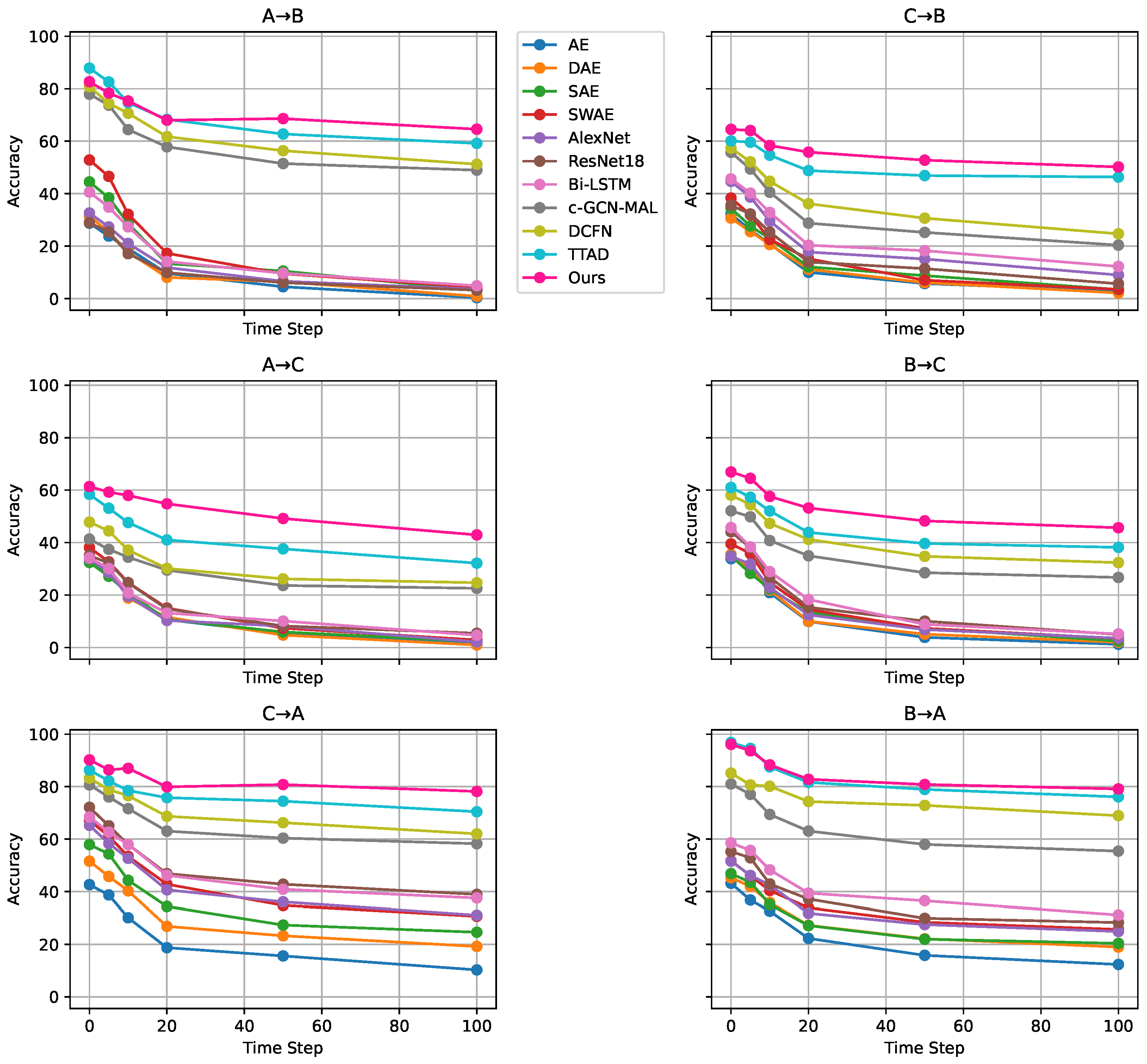
This noise model in Equation (13) captures scenarios where collected signals are influenced by potential changes in the bearing’s internal properties and external operating conditions during deployment. This noise is generated using a compound noise model that integrates Gaussian and sinusoidal components, reflecting the spatiotemporal correlations often observed in industrial environments, as opposed to purely random disturbances. We feed one test sample per time step with n t to simulate the real-world industrial environment, and record the testing performance at the 1, 5, 10, 20, 50, 100 steps.
From the simulated industrial environment results in Figure 4, it is evident that the introduction of composite noise—designed to mimic real-world conditions—causes varying degrees of performance fluctuation and degradation over time for all methods. Traditional autoencoder-based methods and baseline CNN/RNN architectures are significantly affected, with accuracy dropping rapidly and fluctuating heavily as time progresses. Even cross-domain enhanced methods such as c-GCN-MAL, DCFN, and TTAD experience notable performance decay under long-term noise interference.
In contrast, the proposed online learning framework maintains stronger noise resistance and stability across the six cross-domain scenarios. For tasks such as A→B and C→A, our method sustains high accuracy even during later time steps when accumulated noise becomes more severe. In more challenging settings like B→C and C→B, the decline rate of our method’s accuracy is slower than that of all baselines. This robustness is mainly attributed to the ScoreODS-based real-time monitoring of distribution shift and the incremental fine-tuning mechanism using synthesized fault samples, which enable the model to remain adaptive and maintain strong generalization capability under persistent noise disturbances. These results indicate that our method is well-suited not only for static cross-domain fault diagnosis but also for dynamically evolving industrial environments.

4.6. Impact of Hyperparameters in the Loss Function

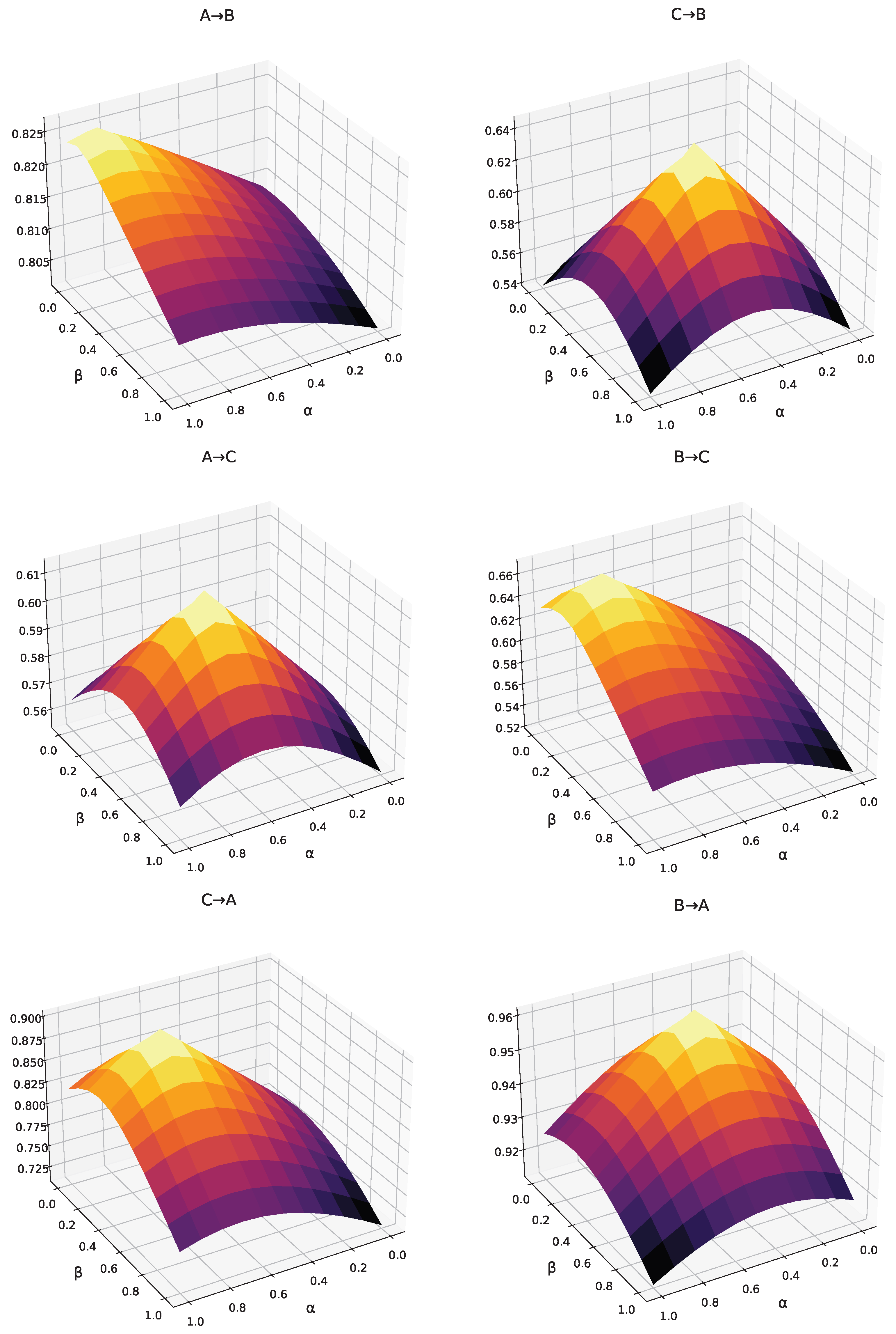
Figure 5 illustrates the impact of the weighting coefficients α and β in Equation (11) on the overall diagnostic performance. Across different cross-domain tasks, a similar trend is observed: when either α or β is set too low or too high, performance degrades; optimal accuracy is achieved when both take moderate values.
Specifically, α controls the relative importance of the generator and discriminator in adversarial training. When α is too small, the discriminator’s constraints are insufficient, leading to lower-quality generated fault samples, which weakens adaptation performance. Conversely, a very large α biases adversarial training toward the discriminator, causing training instability and reducing the realism of generated features. β determines the strength of the classification constraint within the generator. If β is too small, the class separability of generated samples decreases; if β is too large, the generator may overfit the classification task at the expense of diversity in generated data.
Experimental results show that, in our setting, placing both α and β within a moderate range (e.g., 0.4–0.6) yields the best and most stable performance in most tasks. For example, in B→A and C→A tasks, the highest accuracy is attained within this range, with minimal fluctuations. This analysis confirms that both the quality and class discriminability of generated samples play a critical role in effective online adaptation, and provides practical guidance for hyperparameter selection in real-world deployments.

4.7. Effectiveness of ScoreODS

To assess the effectiveness of ScoreODS in detecting distribution drift, we conduct experiments under both noise perturbation and cross-domain adaptation scenarios. For each test sample, we computed the corresponding ScoreODS value and reported the average over the entire test dataset under each experimental condition.
The experimental results in Table 4 demonstrate that the proposed ScoreODS metric is sensitive to distribution shifts. In the noise sensitivity experiments, Gaussian noise of varying intensities ( σ = 0.01, 0.05, 0.10) was injected into the test data. At the lowest noise level, ScoreODS values across all datasets remained close to 1.0 (e.g., A: 1.02 ± 0.05, B: 1.01 ± 0.04, C: 1.03 ± 0.05), indicating that the online data distribution was highly consistent with the offline baseline. As the noise level increased, ScoreODS rose steadily—for instance, in dataset A from 1.02 to 1.15 and 1.30—quantifying the growing deviation in feature space. This confirms that ScoreODS reacts proportionally to noise-induced shifts and can serve as a reliable signal for drift detection.
In the cross-domain adaptation setting, ScoreODS values are substantially above 1, reflecting greater domain discrepancies between the source and target datasets. The A→C task shows the largest drift (1.60 ± 0.15), followed by B→C (1.55 ± 0.14) and C→A (1.50 ± 0.13), indicating considerable difficulty in adaptation. In contrast, tasks such as B→A yield lower values (1.40 ± 0.10), suggesting a milder distribution shift.
Overall, the proposed metric not only tracks domain shifts accurately in static cross-domain settings but also quantifies drift under dynamic, noisy industrial conditions. Its proven effectiveness under both slight perturbation and major domain shifts makes it a robust and practical component for real-time drift detection and adaptive updating in online rolling bearing fault diagnosis.

5. Conclusions and Future Work

This paper proposed an online learning framework for rolling bearing fault diagnosis that adapts to distribution shifts using only normal-condition data during deployment. By combining generative–discriminative fault sample synthesis with the ScoreODS-based drift monitoring mechanism, the method enables adaptive fine-tuning without real fault data. Experiments on public and private datasets demonstrated consistently higher accuracy and stronger robustness than existing baselines, particularly under challenging cross-domain and noisy industrial scenarios.
Future work will focus on extending the framework to multi-sensor fusion and self-supervised representation learning for better domain adaptability, and on enhancing ScoreODS with predictive drift modeling for proactive adaptation in industrial scenarios.

6. Limitations

Despite its strong performance, the proposed approach still involves certain limitations, such as additional computational overhead during online updating, which may affect real-time feasibility on edge devices. Therefore, further optimization and lightweight network design will be explored to improve efficiency in practical deployment.
In addition, although the WAGN-GP generator enables domain consistency to be appoximated by minimizing the Wasserstein distance between the normal and fault sample distributions, the framework still faces inherent limitations. The generator is initially trained with limited fault data and, despite online fine-tuning with newly acquired normal samples, the diversity of generated fault samples remains partially constrained by the scarcity of real fault instances. This limitation may affect the representativeness of the generated fault domain under rapidly changing operating conditions. Moreover, the proposed method is primarily designed to handle gradual or moderate distribution shifts, such as device aging or environmental variations. In scenarios involving extreme domain shifts, re-collecting data and retraining may be required, which is time-consuming and labor-intensive. Nonetheless, many practical domain changes are less severe, and our approach provides a lightweight solution to mitigate performance degradation.

Author Contributions

Methodology, W.L. and J.C.; Validation, W.L. and J.L.; Formal analysis, W.L. and J.C.; Investigation, Y.C.; Resources, Y.W. and J.L.; Data curation, W.L. and Y.W.; Writing—original draft, W.L.; Writing—review & editing, Z.H. and J.C.; Supervision, J.L.; Project administration, J.L.; Funding acquisition, J.C. All authors have read and agreed to the published version of the manuscript.

Funding

This research was supported by the Anhui Provincial Department of Science and Technology under the project “On-board Fault Monitoring and Warning System for High-Speed Railway Operation Safety Based on Acoustic and Vibration Signal Feature Recognition” (No. 711285818079), and by the National Natural Science Foundation of China (No. 62101173).

Data Availability Statement

This study employed both publicly available and private datasets for experimental analyses. The publicly available datasets include Case Western Reserve University (CWRU) Bearing Dataset (https://engineering.case.edu/bearingdatacenter, accessed on 1 March 2025) and Mechanical Failures Prevention Group (MFPT) Bearing Dataset (https://www.kaggle.com/datasets/emperorpein/mfpt-fault-datasets, accessed on 1 March 2025). In addition, a private dataset was collected using a custom experimental platform developed at Hefei University of Technology. Due to copyright and ownership restrictions, this dataset is not publicly available but can be provided upon reasonable request from the corresponding author.

Conflicts of Interest

The authors declare no conflicts of interest.

References

  1. Peng, B.; Bi, Y.; Xue, B.; Zhang, M.; Wan, S. A survey on fault diagnosis of rolling bearings. Algorithms 2022, 15, 347. [Google Scholar] [CrossRef]
  2. Pei, X.; Su, S.; Jiang, L.; Chu, C.; Gong, L.; Yuan, Y. Research on rolling bearing fault diagnosis method based on generative adversarial and transfer learning. Processes 2022, 10, 1443. [Google Scholar] [CrossRef]
  3. Jia, S.; Li, Y.; Wang, X.; Sun, D.; Deng, Z. Deep causal factorization network: A novel domain generalization method for cross-machine bearing fault diagnosis. Mech. Syst. Signal Process. 2023, 192, 110228. [Google Scholar] [CrossRef]
  4. Hakim, M.; Omran, A.A.B.; Ahmed, A.N.; Al-Waily, M.; Abdellatif, A. A systematic review of rolling bearing fault diagnoses based on deep learning and transfer learning: Taxonomy, overview, application, open challenges, weaknesses and recommendations. Ain Shams Eng. J. 2023, 14, 101945. [Google Scholar] [CrossRef]
  5. Zhang, M.; Marklund, H.; Dhawan, N.; Gupta, A.; Levine, S.; Finn, C. Adaptive risk minimization: Learning to adapt to domain shift. Adv. Neural Inf. Process. Syst. 2021, 34, 23664–23678. [Google Scholar]
  6. Zhang, Y.; Ren, Z.; Zhou, S.; Feng, K.; Yu, K.; Liu, Z. Supervised contrastive learning-based domain adaptation network for intelligent unsupervised fault diagnosis of rolling bearing. IEEE/ASME Trans. Mechatronics 2022, 27, 5371–5380. [Google Scholar] [CrossRef]
  7. Zhang, Y.; Ji, J.; Ren, Z.; Ni, Q.; Gu, F.; Feng, K.; Yu, K.; Ge, J.; Lei, Z.; Liu, Z. Digital twin-driven partial domain adaptation network for intelligent fault diagnosis of rolling bearing. Reliab. Eng. Syst. Saf. 2023, 234, 109186. [Google Scholar] [CrossRef]
  8. Yu, X.; Wang, Y.; Liang, Z.; Shao, H.; Yu, K.; Yu, W. An adaptive domain adaptation method for rolling bearings’ fault diagnosis fusing deep convolution and self-attention networks. IEEE Trans. Instrum. Meas. 2023, 72, 3509814. [Google Scholar] [CrossRef]
  9. Wu, Z.; Jiang, H.; Zhu, H.; Wang, X. A knowledge dynamic matching unit-guided multi-source domain adaptation network with attention mechanism for rolling bearing fault diagnosis. Mech. Syst. Signal Process. 2023, 189, 110098. [Google Scholar] [CrossRef]
  10. Zheng, H.; Yang, Y.; Yin, J.; Li, Y.; Wang, R.; Xu, M. Deep domain generalization combining a priori diagnosis knowledge toward cross-domain fault diagnosis of rolling bearing. IEEE Trans. Instrum. Meas. 2020, 70, 3501311. [Google Scholar] [CrossRef]
  11. Xie, Y.; Shi, J.; Gao, C.; Yang, G.; Zhao, Z.; Guan, G.; Chen, D. Rolling Bearing Fault Diagnosis Method Based On Dual Invariant Feature Domain Generalization. IEEE Trans. Instrum. Meas. 2024, 73, 3510211. [Google Scholar] [CrossRef]
  12. Song, Y.; Li, Y.; Jia, L.; Zhang, Y. Domain Generalization Combining Covariance Loss with Graph Convolutional Networks for Intelligent Fault Diagnosis of Rolling Bearings. IEEE Trans. Ind. Inform. 2024, 20, 13842–13852. [Google Scholar] [CrossRef]
  13. Zhu, M.; Liu, J.; Hu, Z.; Liu, J.; Jiang, X.; Shi, T. Cloud-Edge Test-Time Adaptation for Cross-Domain Online Machinery Fault Diagnosis via Customized Contrastive Learning. Adv. Eng. Inform. 2024, 61, 102514. [Google Scholar] [CrossRef]
  14. Li, W.; Chen, Y.; Li, J.; Wen, J.; Chen, J. Learn Then Adapt: A Novel Test-Time Adaptation Method for Cross-Domain Fault Diagnosis of Rolling Bearings. Electronics 2024, 13, 3898. [Google Scholar] [CrossRef]
  15. Wang, H.; Zheng, J.; Xiang, J. Online bearing fault diagnosis using numerical simulation models and machine learning classifications. Reliab. Eng. Syst. Saf. 2023, 234, 109142. [Google Scholar] [CrossRef]
  16. Xu, Q.; Zhu, B.; Huo, H.; Meng, Z.; Li, J.; Fan, F.; Cao, L. Fault diagnosis of rolling bearing based on online transfer convolutional neural network. Appl. Acoust. 2022, 192, 108703. [Google Scholar] [CrossRef]
  17. Liang, P.; Wang, W.; Yuan, X.; Liu, S.; Zhang, L.; Cheng, Y. Intelligent fault diagnosis of rolling bearing based on wavelet transform and improved ResNet under noisy labels and environment. Eng. Appl. Artif. Intell. 2022, 115, 105269. [Google Scholar] [CrossRef]
  18. Che, C.; Wang, H.; Fu, Q.; Ni, X. Deep transfer learning for rolling bearing fault diagnosis under variable operating conditions. Adv. Mech. Eng. 2019, 11, 1687814019897212. [Google Scholar] [CrossRef]
  19. Wang, Z.; He, X.; Yang, B.; Li, N. Subdomain adaptation transfer learning network for fault diagnosis of roller bearings. IEEE Trans. Ind. Electron. 2021, 69, 8430–8439. [Google Scholar] [CrossRef]
  20. Li, X.; Jiang, H.; Xie, M.; Wang, T.; Wang, R.; Wu, Z. A reinforcement ensemble deep transfer learning network for rolling bearing fault diagnosis with multi-source domains. Adv. Eng. Inform. 2022, 51, 101480. [Google Scholar] [CrossRef]
  21. Huo, C.; Jiang, Q.; Shen, Y.; Zhu, Q.; Zhang, Q. Enhanced transfer learning method for rolling bearing fault diagnosis based on linear superposition network. Eng. Appl. Artif. Intell. 2023, 121, 105970. [Google Scholar] [CrossRef]
  22. Ma, L.; Jiang, B.; Xiao, L.; Lu, N. Digital twin-assisted enhanced meta-transfer learning for rolling bearing fault diagnosis. Mech. Syst. Signal Process. 2023, 200, 110490. [Google Scholar] [CrossRef]
  23. Hoi, S.C.; Sahoo, D.; Lu, J.; Zhao, P. Online learning: A comprehensive survey. Neurocomputing 2021, 459, 249–289. [Google Scholar] [CrossRef]
  24. Bhatia, S.; Jain, A.; Srivastava, S.; Kawaguchi, K.; Hooi, B. Memstream: Memory-based streaming anomaly detection. In Proceedings of the ACM Web Conference, Lyon, France, 25–29 April 2022; pp. 610–621. [Google Scholar]
  25. Yang, H.; Qiu, R.C.; Shi, X.; He, X. Unsupervised feature learning for online voltage stability evaluation and monitoring based on variational autoencoder. Electr. Power Syst. Res. 2020, 182, 106253. [Google Scholar] [CrossRef]
  26. Chua, A.; Jordan, M.I.; Muller, R. SOUL: An energy-efficient unsupervised online learning seizure detection classifier. IEEE J. Solid-State Circuits 2022, 57, 2532–2544. [Google Scholar] [CrossRef]
  27. Chen, Z.; Fan, Z.; Chen, Y.; Zhu, Y. Camera-aware cluster-instance joint online learning for unsupervised person re-identification. Pattern Recognit. 2024, 151, 110359. [Google Scholar] [CrossRef]
  28. Alam, M.S.; Yakopcic, C.; Hasan, R.; Taha, T.M. Memristor-Based Neuromorphic System for Unsupervised Online Learning and Network Anomaly Detection on Edge Devices. Information 2025, 16, 222. [Google Scholar] [CrossRef]
  29. Gulrajani, I.; Ahmed, F.; Arjovsky, M.; Dumoulin, V.; Courville, A.C. Improved training of wasserstein gans. In Proceedings of the Advances in Neural Information Processing Systems (NeurIPS), Long Beach, CA, USA, 4–9 December 2017; Volume 30. [Google Scholar]
  30. Kingma, D.P.; Welling, M. Auto-Encoding Variational Bayes. In Proceedings of the 2nd International Conference on Learning Representations (ICLR), Banff, AB, Canada, 14–16 April 2014. [Google Scholar]
  31. Ho, J.; Jain, A.; Abbeel, P. Denoising Diffusion Probabilistic Models. In Proceedings of the Advances in Neural Information Processing Systems, Virtual, 6–12 December 2020; Larochelle, H., Ranzato, M., Hadsell, R., Balcan, M., Lin, H., Eds.; Curran Associates, Inc.: Red Hook, NY, USA, 2020; Volume 33, pp. 6840–6851. [Google Scholar]
  32. Karras, T.; Laine, S.; Aila, T. A Style-Based Generator Architecture for Generative Adversarial Networks. In Proceedings of the IEEE/CVF Conference on Computer Vision and Pattern Recognition (CVPR), Long Beach, CA, USA, 16–20 June 2019. [Google Scholar]
  33. Baldi, P. Autoencoders, unsupervised learning and deep architectures. In Proceedings of the International Conference on Unsupervised and Transfer Learning Workshop, Bellevue, WA, USA, 10–15 July 2012; Volume 27, pp. 37–49. [Google Scholar]
  34. Rumelhart, D.E.; Hinton, G.E.; Williams, R.J. Learning internal representations by error propagation. In Parallel Distributed Processing: Explorations in the Microstructure of Cognition, Vol. 1: Foundations; MIT Press: Cambridge, MA, USA, 1986; pp. 318–362. [Google Scholar]
  35. Vincent, P.; Larochelle, H.; Bengio, Y.; Manzagol, P.A. Extracting and composing robust features with denoising autoencoders. In Proceedings of the 25th International Conference on Machine Learning, New York, NY, USA, 5–9 July 2008; pp. 1096–1103. [Google Scholar]
  36. Ranzato, M.; Poultney, C.; Chopra, S.; LeCun, Y. Efficient learning of sparse representations with an energy-based model. In Proceedings of the 19th International Conference on Neural Information Processing Systems, Vancouver, BC, Canada, 4–9 December 2006; pp. 1137–1144. [Google Scholar]
  37. Sun, S.; Guo, H. Symmetric Wasserstein Autoencoders. In Proceedings of the Uncertainty in Artificial Intelligence (UAI), Virtual, 17–20 August 2021; pp. 354–364. [Google Scholar]
  38. Krizhevsky, A.; Sutskever, I.; Hinton, G.E. ImageNet classification with deep convolutional neural networks. Commun. ACM 2012, 60, 84–90. [Google Scholar] [CrossRef]
  39. He, K.; Zhang, X.; Ren, S.; Sun, J. Deep Residual Learning for Image Recognition. In Proceedings of the 2016 IEEE Conference on Computer Vision and Pattern Recognition (CVPR), Las Vegas, NV, USA, 27–30 June 2016; pp. 770–778. [Google Scholar]
  40. Huang, Z.; Xu, W.; Yu, K. Bidirectional LSTM-CRF Models for Sequence Tagging. arXiv 2015, arXiv:1508.01991. [Google Scholar] [CrossRef]
  41. Wen, H.; Guo, W.; Li, X. A novel deep clustering network using multi-representation autoencoder and adversarial learning for large cross-domain fault diagnosis of rolling bearings. Expert Syst. Appl. 2023, 225, 120066. [Google Scholar] [CrossRef]
  42. Glorot, X.; Bengio, Y. Understanding the difficulty of training deep feedforward neural networks. In Proceedings of the Artificial Intelligence and Statistics, Sardinia, Italy, 13–15 May 2010; pp. 1–8. [Google Scholar]
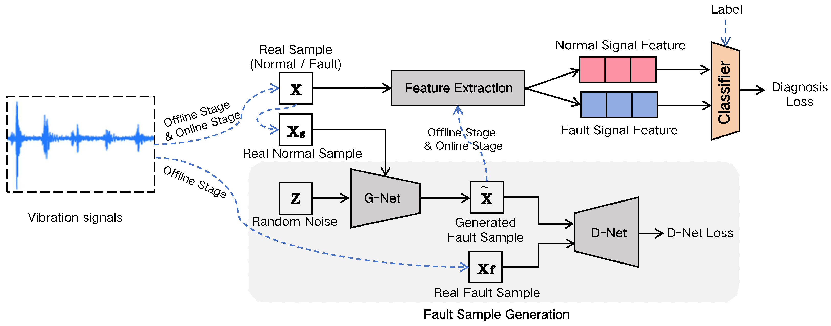
Figure 1. The framework of our proposed method.
Mathematics 13 03763 g001
Figure 2. The architecture of Encoder, where raw vibration signals are encoded as signal embeddings.
Mathematics 13 03763 g002
Figure 3. The aero-engine bearing test bench of the private dataset in Hefei University of Technology: (a) the components of the test bench and (b) accelerometer measurement locations.
Mathematics 13 03763 g003
Figure 4. Performance comparison under simulated industrial environment.
Mathematics 13 03763 g004
Figure 5. The impacts of various values of the parameters α and β in all cases. The Z-axis represents the overall accuracy. The color gradient ranges from purple (lower accuracy) to yellow (higher accuracy), illustrating the performance variation across different parameter combinations.
Mathematics 13 03763 g005
Table 1. Comparison of cross-domain learning paradigms for fault diagnosis.
ParadigmSource LabelsTarget LabelsAdaptation StageKey CharacteristicsWeaknesses
Transfer Learning✔/×TrainingFine-tuning of pretrained models; access limited target dataSensitive to domain shift; overfits when target data is limited
Domain Adaptation×TrainingUnsupervised domain alignment using unlabeled dataSensitive to sensor noise; adaptation speed is limited
Domain Generalization✔ *×None (Zero-shot)Learns domain-invariant features from multiple source domainsPerformance drops on unseen operating conditions; less robust to sudden faults
Test-Time Adaptation×Test-timeAdapts online with unlabeled target data during inferenceHigh computational overhead during inference; sensitive to noisy input
Online Learning✔/×Continuous (streaming)Incremental model updates with continuously arriving target dataProne to catastrophic forgetting; adaptation speed constrained by model complexity
* DG generally assumes multiple source domains to enhance generalization. ✔ and × indicate the presence and absence of labels, respectively.
Table 2. The diagnosis accuracies (%) comparison with various baselines and three datasets under the cross-domain setting. The arrow → represents the adaptation from the source domain to the target domain. To ensure the reliability of experimental results, we test each baseline five times and take the average value.
DatasetAEDAESAESWAEAlex-NetRes-Net18Bi-LSTMc-GCN-MALDCFNTTADOurs
A→B28.74  ± 0.731.46  ± 1.344.47  ± 0.952.82  ± 1.132.62  ± 0.228.93  ± 1.840.58  ± 0.477.90  ± 0.180.78  ± 1.687.86  ± 1.282.66  ± 0.4
A→C33.33  ± 0.333.60  ± 1.732.43  ± 0.838.13  ± 0.533.87  ± 1.935.06  ± 0.634.18  ± 0.441.33  ± 1.547.81  ± 0.958.39  ± 0.761.37  ± 1.0
B→A43.16  ± 0.245.26  ± 1.846.84  ± 0.351.73  ± 0.651.58  ± 1.455.26  ± 0.158.55  ± 1.181.01  ± 0.885.16  ± 1.396.84  ± 0.596.12  ± 0.3
B→C33.87  ± 0.235.48  ± 1.934.87  ± 0.739.49  ± 0.434.76  ± 1.044.12  ± 0.345.74  ± 1.552.12  ± 0.958.07  ± 0.861.02  ± 1.766.94  ± 1.5
C→A42.63  ± 0.651.58  ± 1.657.89  ± 0.567.14  ± 1.265.26  ± 0.172.11  ± 1.468.42  ± 0.980.67  ± 0.383.24  ± 1.886.32  ± 1.390.20  ± 1.1
C→B32.23  ± 1.530.68  ± 0.634.37  ± 1.138.33  ± 0.844.66  ± 1.935.53  ± 0.345.63  ± 1.755.74  ± 0.257.33  ± 1.060.10  ± 0.564.51  ± 0.7
Table 3. The diagnosis F1-scores (%) comparison with various baselines and three datasets under the cross-domain setting. The arrow → represents the adaptation from the source domain to the target domain.
DatasetAEDAESAESWAEAlex-NetRes-Net18Bi-LSTMc-GCN-MALDCFNTTADOurs
A→B26.17  ± 0.627.83  ± 1.241.58  ± 0.850.76  ± 1.030.97  ± 0.226.35  ± 1.7636.77  ± 0.375.34  ± 0.179.16  ± 1.5786.10  ± 1.181.00  ± 0.3
A→C30.66  ± 0.230.93  ± 1.630.78  ± 0.735.37  ± 0.430.19  ± 1.832.36  ± 0.531.50  ± 0.340.50  ± 1.446.86  ± 0.857.22  ± 0.660.14  ± 0.9
B→A41.30  ± 0.241.35  ± 1.742.90  ± 0.248.69  ± 0.548.55  ± 1.353.15  ± 0.155.38  ± 1.078.39  ± 0.783.46  ± 1.294.90  ± 0.494.20  ± 0.2
B→C29.19  ± 0.231.77  ± 1.833.17  ± 0.635.70  ± 0.332.07  ± 0.941.24  ± 0.242.83  ± 1.450.08  ± 0.856.91  ± 0.758.80  ± 1.665.60  ± 1.4
C→A38.78  ± 0.546.55  ± 1.554.73  ± 0.463.80  ± 1.160.95  ± 0.168.67  ± 1.365.06  ± 0.876.06  ± 0.281.57  ± 1.784.59  ± 1.288.40  ± 1.0
C→B31.58  ± 1.430.07  ± 0.533.68  ± 1.037.56  ± 0.743.77  ± 1.834.82  ± 0.244.71  ± 1.654.62  ± 0.256.18  ± 0.958.90  ± 0.463.22  ± 0.6
Table 4. ScoreODS under different experimental conditions. Values are mean ± standard deviation. For Noise Sensitivity, Δ indicates the increase relative to the lowest noise level (0.01). ScoreODS 1 indicates stable distribution; larger values indicate stronger domain shift or noise effect.
Dataset/Source→TargetNoiseScoreODS Δ
Noise Sensitivity
AGaussian 0.011.02  ±  0.050.00
AGaussian 0.051.15  ±  0.07+0.13
AGaussian 0.101.30  ±  0.10+0.28
BGaussian 0.011.01  ±  0.040.00
BGaussian 0.051.12  ±  0.06+0.11
BGaussian 0.101.28  ±  0.09+0.27
CGaussian 0.011.03  ±  0.050.00
CGaussian 0.051.17  ±  0.08+0.14
CGaussian 0.101.32  ±  0.11+0.29
Domain Shift
A → B-1.45  ±  0.12-
A → C-1.60  ±  0.15-
B → A-1.40  ±  0.10-
B → C-1.55  ±  0.14-
C → A-1.50  ±  0.13-
C → B-1.48  ±  0.12-
Disclaimer/Publisher’s Note: The statements, opinions and data contained in all publications are solely those of the individual author(s) and contributor(s) and not of MDPI and/or the editor(s). MDPI and/or the editor(s) disclaim responsibility for any injury to people or property resulting from any ideas, methods, instructions or products referred to in the content.