Improving the Performance of Static Malware Classification Using Deep Learning Models and Feature Reduction Strategies

Abstract

The rapid evolution of malware continues to pose severe challenges to cybersecurity, highlighting the need for accurate and efficient detection systems. Traditional signature- and heuristic-based methods are increasingly inadequate against sophisticated threats, which has motivated the use of machine learning and deep learning for static malware classification. In this study, we propose three deep neural network (DNN) architectures tailored for the binary classification of Portable Executable (PE) files. The models were trained and validated on the EMBER 2017 dataset and further tested on the independent REWEMA dataset to evaluate their cross-dataset generalization capabilities. To address the computational burden of high-dimensional feature vectors, two feature reduction strategies were examined: the Kumar method, which selected 276 features, and the LightGBM-based intersection method, which identified 206 shared features. Experimental results showed that the proposed Model III consistently achieved the best overall performance, outperforming LightGBM (v3.3.5) and the other DNN models in terms of accuracy, recall, and F1-score. Notably, its recall exceeded that of LightGBM by 0.73%, highlighting its superiority in reducing false negative rates. Feature reduction further demonstrated that significant dimensionality reduction could be achieved without compromising classification quality, with the Kumar method achieving the best balance between accuracy and efficiency. Cross-dataset validation revealed performance degradation across all models due to distributional shifts, but the decline was less significant for the DNNs, confirming its greater adaptability compared with LightGBM. These findings demonstrate that architectural optimization and appropriate feature selection can significantly improve the performance of static malware classification. This study also provides empirical benchmarks and methodological guidance for developing accurate, efficient, and resilient malware detection systems that are resilient to evolving threats.

1. Introduction

The rapid expansion of digital technologies has shifted human activity increasingly toward online spaces, where the Internet has become the dominant medium for communication and information exchange. However, this shift has also created new opportunities for malicious actors, leading to the rise of cybercrime as a significant societal concern. Malware is frequently employed in such attacks to disrupt systems or exfiltrate sensitive data, and it can take diverse forms including viruses, worms, trojans, and ransomware [1].

Over the past two decades, malware detection technologies have undergone a notable evolution. Early defenses relied primarily on signature-driven antivirus software, followed by heuristic-based approaches designed to identify suspicious behaviors. Nevertheless, the increasing complexity, diversity, and sheer volume of malware have exposed the limitations of signature- and heuristic-based analysis, accelerating the transition toward machine-learning-based solutions. For example, Endpoint Detection and Response (EDR) systems have been introduced, which combine software attributes and runtime behaviors with machine learning techniques to enhance detection accuracy [2].

Malware analysis can be broadly categorized into static and dynamic approaches. Dynamic analysis methods monitor runtime behaviors, including API call sequences, memory usage, and network activity [3]. Studies have reported that files containing multiple Portable Executable (PE) headers can indicate maliciousness [4]. Other derived characteristics examined include the number of sections, the presence of specific sections (like reloc) [5], non-standard section counts, and section entropy [6]. Although dynamic approaches can capture behavioral richness, they are resource-intensive and less practical for real-time detection.

Static analysis methods focus on extracting discriminative features from PE files [7] without executing them. Compared to dynamic approaches, static analysis methods are more suitable for early detection, enabling systems to identify threats before malware is executed, thus preventing potential damage. Researchers have demonstrated that header information provides rich attributes sufficient for malware classification [8], utilizing information such as raw byte values from DOS and NT headers combined with embedding layers to reduce dimensionality before clustering [9]. Other works utilized libraries like PortEx to extract header fields and applied algorithms like Extra Trees to compute feature importance for selection [10]. While confirming the potential of PE-based features, these studies also highlight a challenge: the high dimensionality of PE features increases computational costs, motivating the exploration of effective feature reduction strategies. Moreover, existing datasets are often limited in size or accessibility, hindering reproducibility and fair benchmarking.

Addressing these gaps, this study proposed three deep neural network (DNN) architectures tailored for static malware classification. The models were evaluated on the EMBER 2017 dataset [11] and further tested on the REWEMA dataset [12] to assess their cross-dataset generalization capabilities. Moreover, two feature selection strategies—the Kumar method (276 features) and the LightGBM-based intersection method (206 features)—were examined to determine their impact on efficiency and performance.

The main contributions of this work can be summarized as follows:

• Proposing three DNN architectures for static malware classification and demonstrating their effectiveness compared with the LightGBM baseline.
• Validating the models on both the EMBER and REWEMA datasets, thereby assessing their cross-dataset generalization capabilities.
• Investigating feature reduction strategies that balance classification performance and computational efficiency.
• Providing empirical insights to guide the design of practical and adaptable malware detection systems.

2. Related Works

Malware classification has been widely studied, with researchers exploring both traditional machine learning and emerging deep learning approaches. To overcome the limitations of conventional analysis—the high dimensionality and computational burden of static features and the resource intensiveness of dynamic monitoring—current research is increasingly focused on feature selection and deep learning methodologies. Feature selection and dimensionality reduction are critical for retaining only the most informative attributes, leading to more efficient model training. Concurrently, deep learning models have shown robust potential for processing high-dimensional data derived from PE files. This section reviews established approaches for minimizing feature space and summarizes recent advancements in deep learning applied to static malware detection.

Oyama et al. [13] applied clustering and feature selection to reduce dimensionality while retaining performance. Kumar et al. [14] ranked features by importance using XGBoost and identified 276 essential ones, whereas Pham et al. [15] selected 1711 features, surpassing models trained with all 2351 features.

Table 1. Feature Groups of the EMBER Dataset.

Feature Category	Feature Name	Dimension	Description
Statistical Values (Features unrelated to PE format)	ByteHistogram	256	Count of each byte value (0–255) in the file.
	ByteEntropyHistogram	256	Approximation of the joint distribution of entropy and byte value.
	String	104	Statistics regarding printable strings (e.g., length, count, entropy).
PE Header and Generated Numeric Values	GeneralFileInfo	10	General structural information (e.g., file size, virtual size).
	HeaderFileInfo	62	Information extracted from the COFF and Optional headers.
	SectionInfo	255	Properties of sections (e.g., names, sizes, entropy).
	ImportsInfo	1024	Hashed import libraries and functions.
	ExportsInfo	128	Hashed exported functions.
	Total	2351

summarizes the feature groups of the EMBER dataset [16], underscoring the need to identify compact yet informative subsets for efficient training.

Deep learning approaches have been increasingly explored on EMBER. Anderson et al. [16] first released the dataset with LightGBM (v3.3.5) as a baseline. Sumit et al. [17] applied deep neural networks, achieving competitive results. Pramanik et al. [18] further compared fully connected and one-dimensional convolutional models, finding the former superior. As summarized in

Table 2. Comparison of Machine Learning Models Based on the EMBER Dataset.

Reference	Feature Dimensions	Classification Model	Evaluation Metrics
Anderson et al. [16]	2351	LightGBM	ROC AUC
Pham et al. [15]	1711	LightGBM	ROC AUC
Oyama et al. [13]	1957–2351	LightGBM	Accuracy
Kumar et al. [14]	276	XGBoost Gradient Boosted Decision Tree	Accuracy and ROC AUC
Sumit et al. [17]	2381	Deep Neural Network	Accuracy and ROC AUC

, although these deep models and other state-of-the-art (SOTA) approaches (such as image-based Convolutional Neural Networks, or CNNs) demonstrate strong potential, their performance is often sensitive to feature selection and dataset scale.

In summary, prior studies have advanced malware classification through diverse methodologies. However, key challenges remain: many works rely on private datasets, limiting reproducibility; the high dimensionality of PE features continues to pose computational burdens; and cross-dataset generalization is rarely investigated. Addressing these gaps, this study proposed three deep neural network architectures evaluated on EMBER and validated with REWEMA while also examining two feature reduction strategies for balancing efficiency and performance.

3. Materials and Methods

3.1. Research Workflow

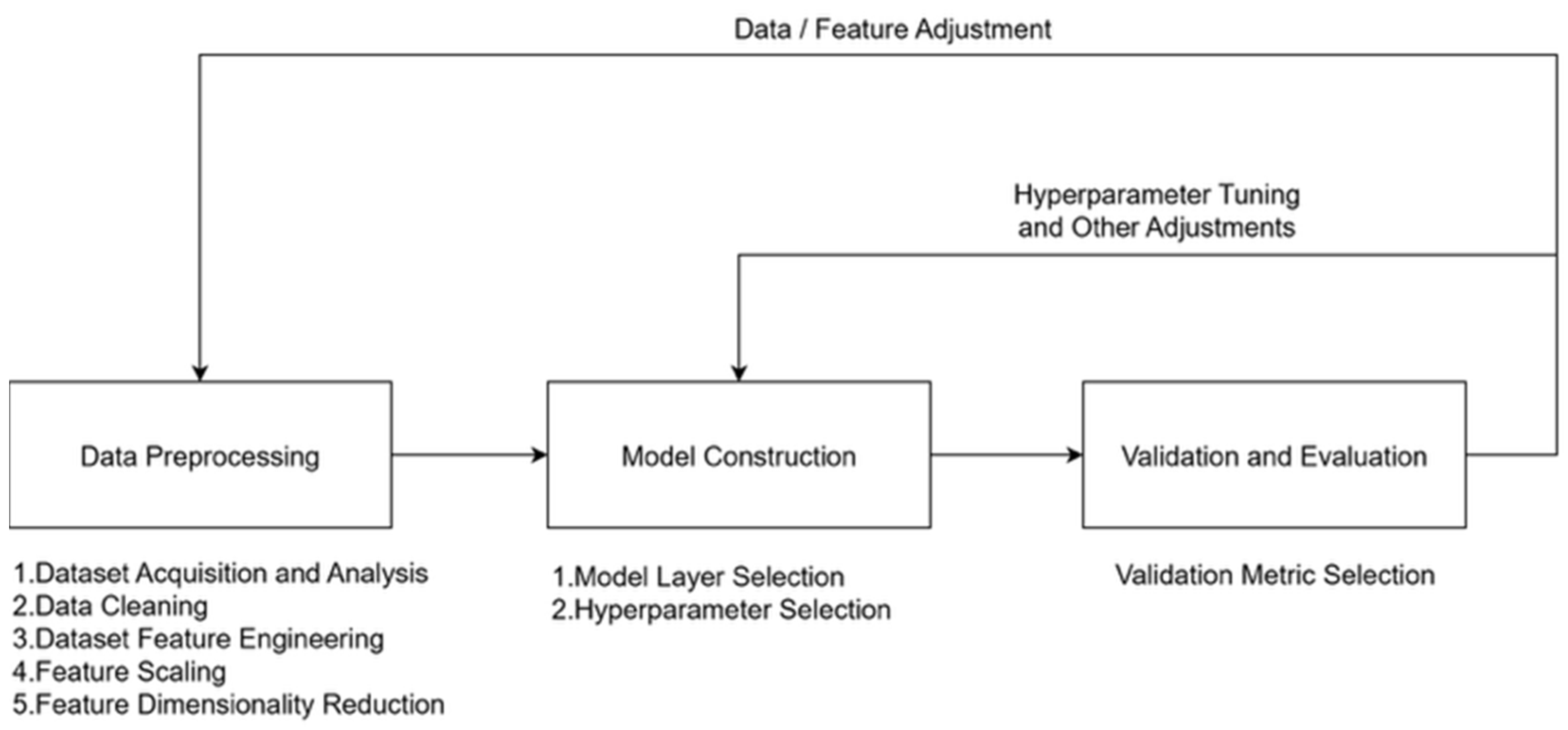
As shown in Figure 1, this study adopted a standardized deep learning development pipeline, which unfolds in three main stages.

The first stage is data preprocessing. In this stage, malware datasets are collected, cleaned, and normalized to remove noise and inconsistencies. Features are then transformed into structured feature vectors, with additional adjustments—such as feature selection or dimensionality reduction—applied when necessary to enhance representational quality.

The second stage is model construction. At this step, different neural network architectures are explored and optimized by tuning critical hyperparameters, including learning rate, batch size, and the number of hidden layers. Such optimization is essential to ensure both stable convergence and strong predictive performance.

The final stage is validation and evaluation. In this phase, the trained models are tested not only on validation splits of the EMBER dataset, but also on an external dataset to assess generalization capability. Key performance metrics—such as accuracy, recall, F1-score, and ROC AUC—are then employed to provide a comprehensive assessment of the models’ effectiveness and robustness.

3.2. Data Preprocessing

Data preprocessing in this study consisted of five steps, as shown in Figure 1. These steps ensure that the raw datasets are transformed into consistent and representative feature vectors suitable for deep learning models.

Step 1: Dataset acquisition and analysis. Malware datasets can be broadly categorized into three types. Public datasets, such as EMBER [16] and the Microsoft Malware Classification Challenge [19], are released by corporations or large research groups and are typically accompanied by detailed documentation and related publications. Semi-public datasets are usually provided by individuals or small teams, for instance, through GitHub repositories or Kaggle competitions. Unlike public datasets, they are rarely cited across multiple studies, raising concerns about reliability and fairness. The third category comprises privately collected datasets, which are curated by research teams for internal use and described only in their publications.

Table 3. Analysis of Advantages and Disadvantages of Dataset Types.

Data Type	Data Category	Advantages	Disadvantages
Public Datasets	Processed Data	Sources are verifiable and reliable. A substantial body of research is based on these datasets.	Feature fields are fixed, offering little flexibility.
Semi-Public Datasets	Processed Data/Raw PE	Sources are diverse. Greater flexibility in feature extraction compared with public datasets.	Often require replication of the original experimental environment. Validation may be complex.
Private Collected Datasets	Raw PE Files	Maximum flexibility in feature extraction and manipulation.	Limited accessibility. High collection difficulty.

compares the strengths and limitations of these dataset types. In this study, we adopted the EMBER 2017 dataset as the primary benchmark to ensure reproducibility and fair evaluation. For pre-processed datasets, documentation and related publications were carefully examined to understand the semantics of each feature. For raw PE files, the relevant attributes were first identified and extracted using tools such as the LIEF Library (v0.9) [20] or IDA (v6.5) [21]. The resulting features were then consolidated into a structured dataset for subsequent steps.

Step 2: Data cleaning. At this stage, irrelevant subsets are removed and missing values are addressed. Because the EMBER dataset contains both labeled and unlabeled samples, all unlabeled entries were discarded to enable supervised deep learning.

Step 3: Dataset feature engineering. Since deep learning fundamentally relies on matrix operations, features must be expressed in structured numerical form. As shown in Table 1, the EMBER dataset includes eight feature groups: Byte Histogram, Byte Entropy Histogram, PE String Features, File Features, Header Features, Section Features, Imported Functions, and Exported Functions. These groups contain both numerical and string attributes. To transform string features into numerical vectors, algorithms such as One-Hot Encoding or Feature Hashing [22] can be applied. In this study, Feature Hashing was selected, as One-Hot Encoding would have caused a dramatic increase in dimensionality due to the large number of imported functions.

Step 4: Feature scaling. Without scaling, extreme values may dominate the training process, while small-valued features may be overshadowed. To mitigate these effects, statistical techniques such as normalization, Z-score standardization, min–max scaling, and max–abs scaling are commonly used. In this study, normalization and Z-score standardization were applied, ensuring that feature distributions are centered at zero with unit variance. This adjustment reduces the influence of outliers and aligns the data with the assumptions underlying many machine learning algorithms.

Step 5: Feature dimensionality reduction. Even after vectorization and scaling, the EMBER dataset remains high-dimensional, with 2351 features. Such dimensionality increases computational cost, slows model training, and may lead to overfitting. Therefore, feature reduction techniques are considered to retain only the most informative attributes while discarding redundant or less significant ones. In later experiments (Section 4.3), we specifically evaluated two strategies: (i) the Kumar method, which selects 276 features based on feature importance ranking, and (ii) the LightGBM intersection method, which identifies 206 features common to multiple ranking criteria. By integrating dimensionality reduction into the preprocessing pipeline, the models achieve more efficient training while preserving competitive accuracy.

3.3. Model Construction

Model construction in this study involved determining both the appropriate neural architecture and the configuration of its parameters. For one-dimensional tensor features, Fully Connected Layers are well-suited, whereas higher-order tensors—such as two- or three-dimensional image data—are more effectively captured using Convolutional Layers. Pramanik et al. [18] evaluated both approaches on the EMBER dataset and found that the Fully Connected model outperformed its one-dimensional convolutional counterpart. Accordingly, this study adopted fully connected architecture as the basis for model design.

Hyperparameter tuning represents another critical aspect of model construction. The parameters considered include the objective function, activation function, optimizer, learning rate, epoch count, and batch size. Since the task is a binary classification of PE files, Binary Cross-Entropy [23] was selected as the loss function. While Vinayakumar et al. reported strong performance using the ReLU activation function on EMBER [24], our experiments demonstrated that replacing ReLU with Swish [25]—particularly within a Self-Normalizing Neural Network (SNN)—achieved superior classification performance.

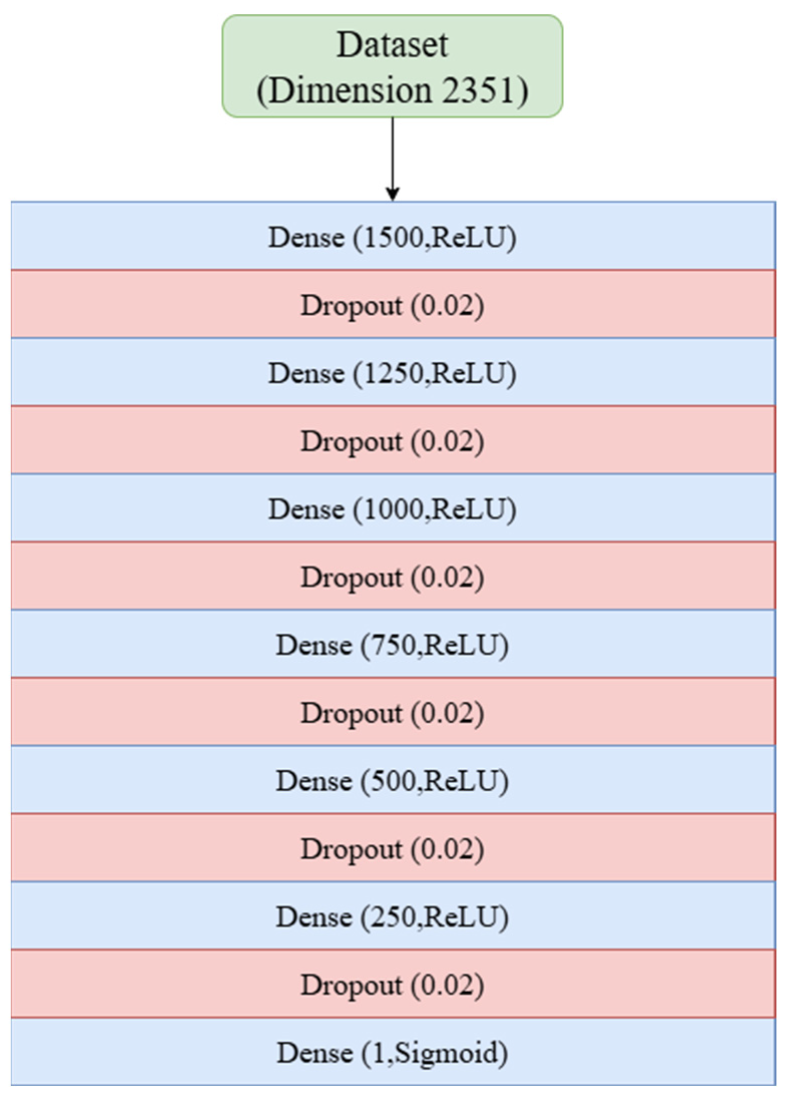
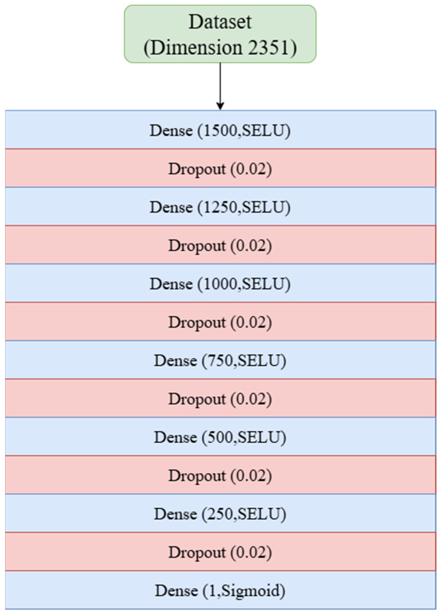
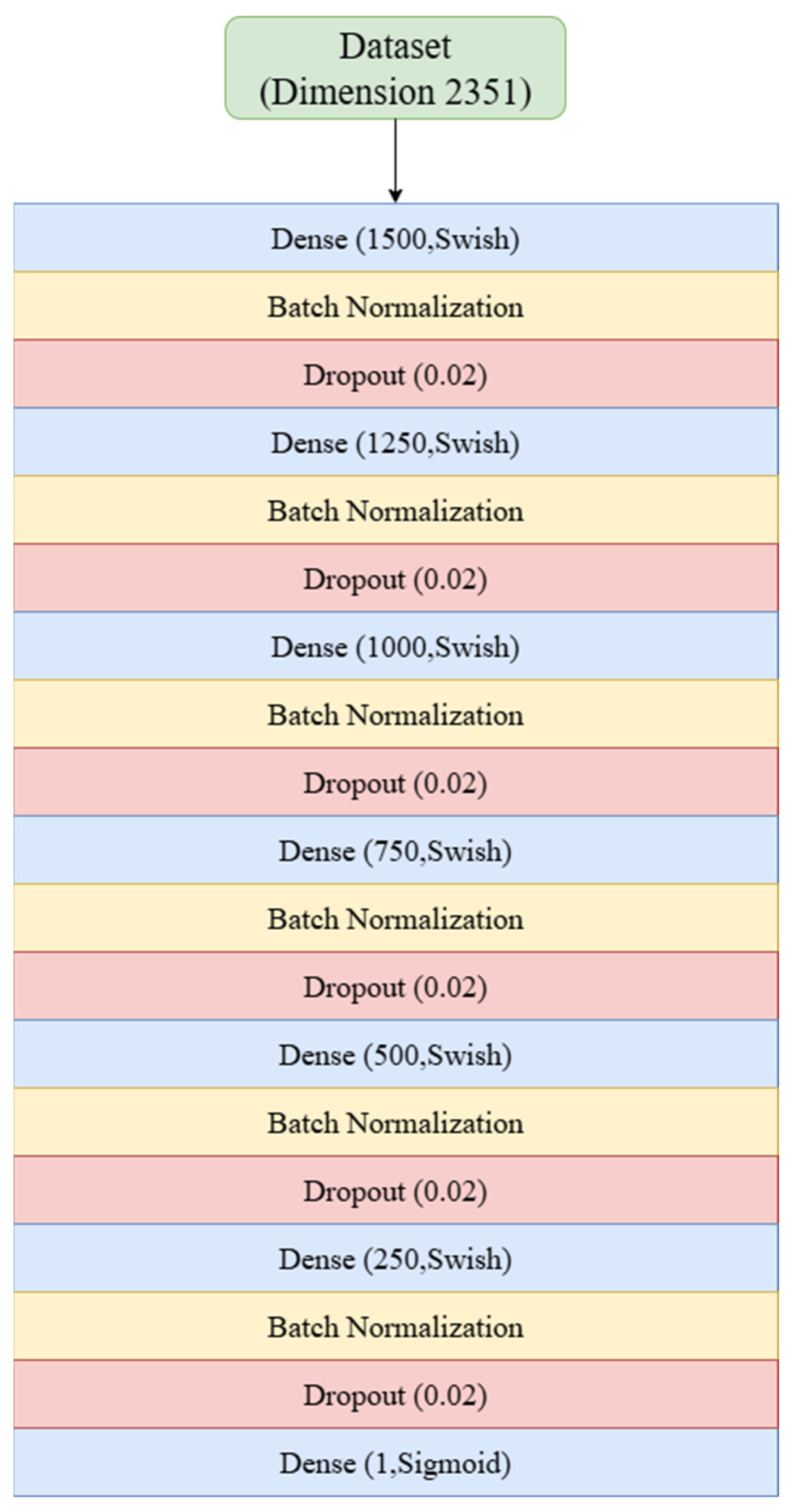
Based on these considerations, three models were developed. Model I extends the framework of Sumit et al. [17] by deepening the network to 13 layers and adjusting dropout rates; cross-validation identified 24 epochs as optimal. Model II modifies Model I into an SNN design by incorporating LecunNormal weight initialization and AlphaDropout, with 24 epochs again selected through cross-validation. Model III also builds on Model I but replaces the ReLU activation with Swish and integrates Batch Normalization Layers; cross-validation determined 30 epochs as optimal for this configuration.

Across all three models, a consistent set of hyperparameters was applied: Binary Cross-Entropy as the loss function, Adam [26] as the optimizer, a learning rate of 0.001, a batch size of 256, Sigmoid activation in the output layer, and fivefold cross-validation.

For clarity, the corresponding architectures and parameter settings of Models I, II, and III are presented in Appendix A (Figure A1, Figure A2 and Figure A3). These figures illustrate the complete layer configurations and hyperparameter choices for each model. In addition,

Table 4. Comparative summary of the proposed deep learning models.

Model	Base Architecture	Activation Function	Normalization & Regularization	Optimal Epochs
Model I	Extended Sumit et al. [17] (13 layers)	ReLU	Dropout (0.02)	24
Model II	Self-Normalizing Network (SNN)	SELU	AlphaDropout (0.02) + LecunNormal Init.	24
Model III	Optimized DNN	Swish	Batch Normalization + Dropout (0.02)	30

provides a comparative summary of the three models, highlighting their architectural modifications and the optimal number of training epochs identified through cross-validation. Together, these materials provide both detailed specifications and a concise overview of the proposed designs.

3.4. Validation and Evaluation

The final stage focuses on model evaluation. In binary classification, performance is typically assessed using several standard metrics, including Accuracy, Recall, Precision, F1 Score, and the Area Under the Receiver Operating Characteristic Curve (ROC AUC) [27]. Each captures a distinct aspect of model behavior: Accuracy reflects the overall proportion of correctly classified samples; Recall measures the ability to detect malicious cases; Precision indicates the reliability of positive predictions; the F1 Score balances Precision and Recall in a single indicator; and ROC AUC summarizes the model’s discriminative capability across different decision thresholds.

In this study, Precision, Recall, F1 Score, and ROC AUC were adopted as the primary evaluation criteria, while Accuracy was additionally reported to facilitate comparison with prior work. This combination of metrics provides a balanced perspective, ensuring that the proposed models are not only effective in detecting malicious software, but also robust in minimizing false alarms. For benchmarking purposes, the performance of our models was directly compared with the LightGBM model reported by Anderson et al. [16] and the deep learning model presented by Sumit et al. [17]. This alignment with established baselines positions our results within the broader EMBER-based malware classification literature and enables a fair and transparent evaluation.

4. Results

4.1. Experimental Environment and Datasets

The experiments in this study were conducted on a standard workstation serving as the platform for model construction, training, and evaluation. The system was equipped with a 12th-generation Intel Core i9-12900K processor (Intel Corporation, Taiwan), 48 GB of RAM (Kingston, Taiwan), and an NVIDIA GeForce RTX 3080 Ti graphics card with 12 GB of dedicated memory (MSI, Taiwan). Although this configuration does not constitute a high-performance computing cluster, it was sufficient to support both traditional machine learning methods and the deep neural networks developed in this work.

To ensure fairness in benchmarking and comparability with prior studies, we adopted the EMBER 2017 (version 1, v1) dataset [11] as the primary benchmark. This was a deliberate methodological choice to ensure a fair and direct comparison against the foundational models against which we benchmarked, including the original LightGBM [16] and the DNN models proposed by Sumit et al. [17], all of which utilized the v1 dataset. The dataset is extensive, containing 300,000 malicious and 300,000 benign training samples, 300,000 unlabeled training samples, 100,000 malicious, and 100,000 benign testing samples. For the proposed deep learning models, only labeled data were retained, while all unlabeled samples were removed during preprocessing to maintain consistency with supervised learning.

To further assess the generalization capability of the proposed models, we incorporated the REWEMA dataset [12] as an independent test set. Unlike EMBER, which provides pre-processed feature vectors, REWEMA consists of raw PE files (executables). It contains 3136 benign and 3104 malicious samples, totaling 6240 files. Feature engineering was therefore required to extract vectors consistent with the feature fields and dimensionality defined in the EMBER dataset. This alignment ensured that cross-dataset comparisons remained meaningful and reliable, thus enabling a fair evaluation of model generalization. It is important to note that both the EMBER and REWEMA datasets are balanced, with a benign-to-malicious ratio of approximately 1:1. Therefore, techniques for handling imbalanced data were not required for this study.

4.2. Model Training and Performance Comparison

We first conducted a comparative evaluation of machine learning and deep learning models using the EMBER dataset under identical experimental conditions. To identify the optimal number of training epochs for each model, fivefold cross-validation was employed. This procedure enabled the performance metrics to be averaged across folds at different epochs and based on these results, to determine the epoch that yielded the best overall performance.

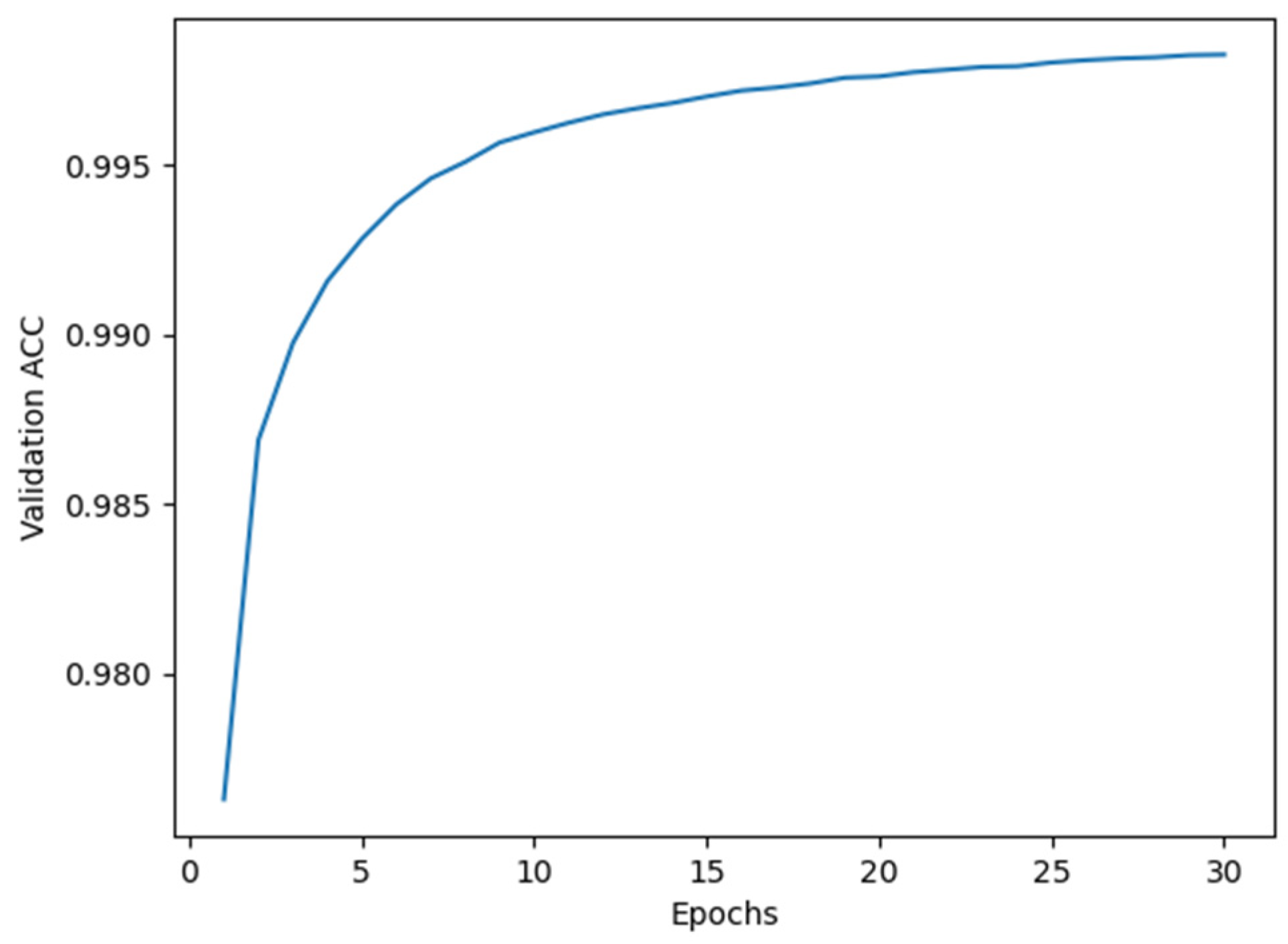
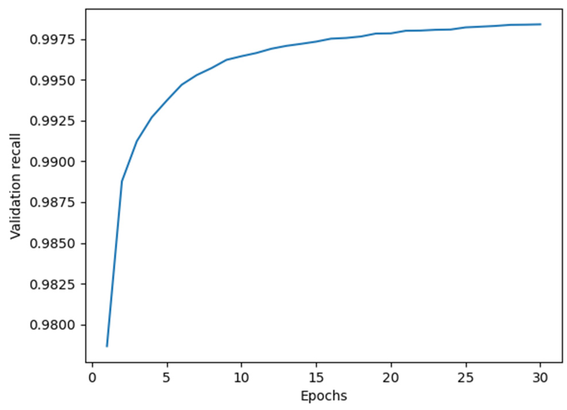
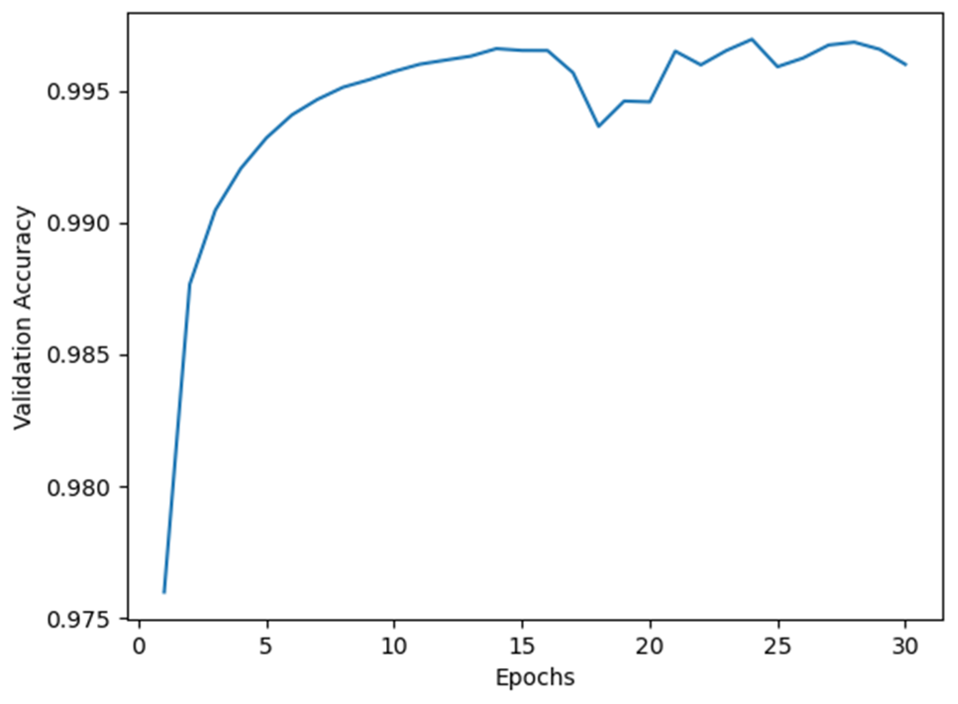
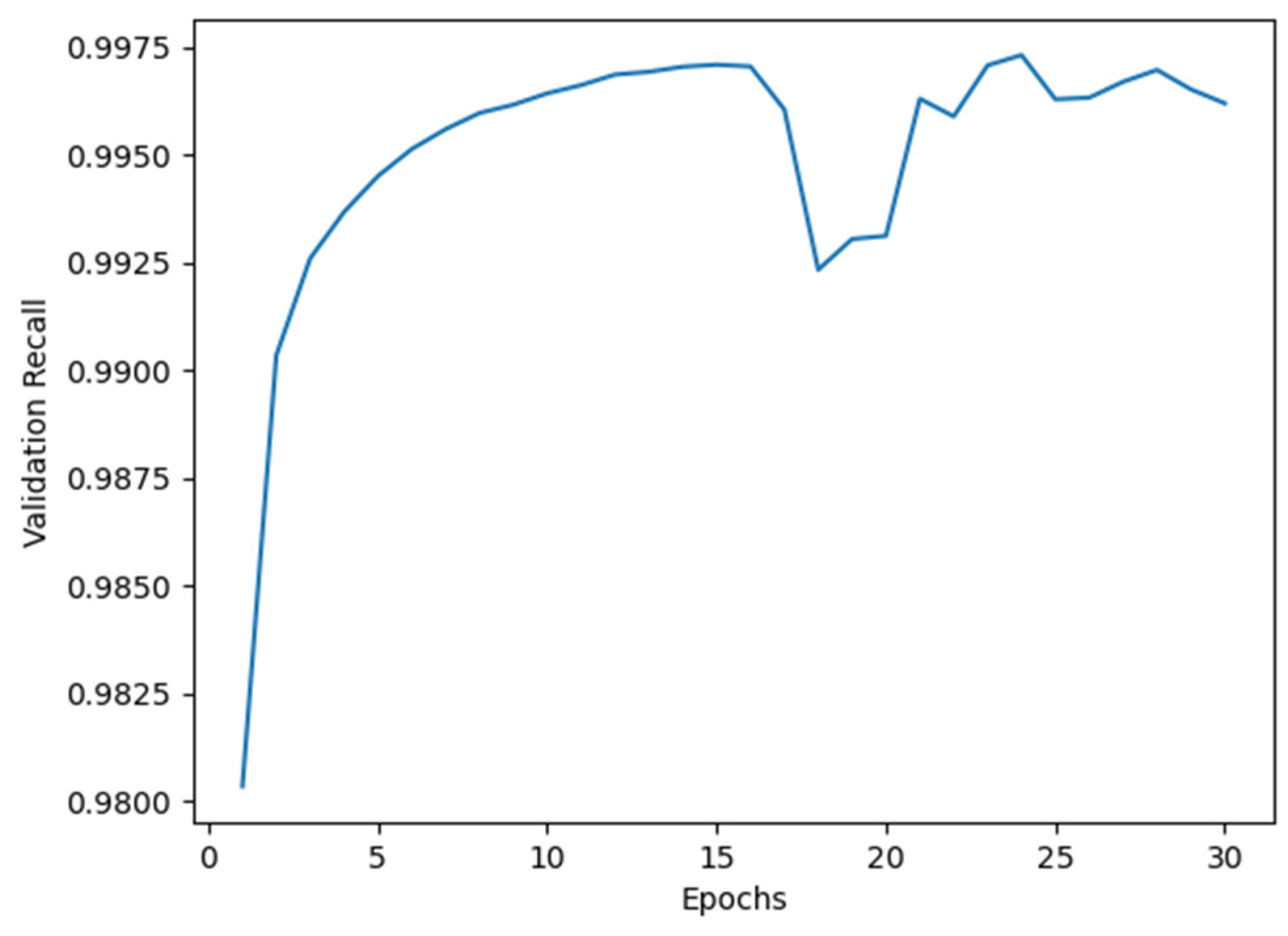
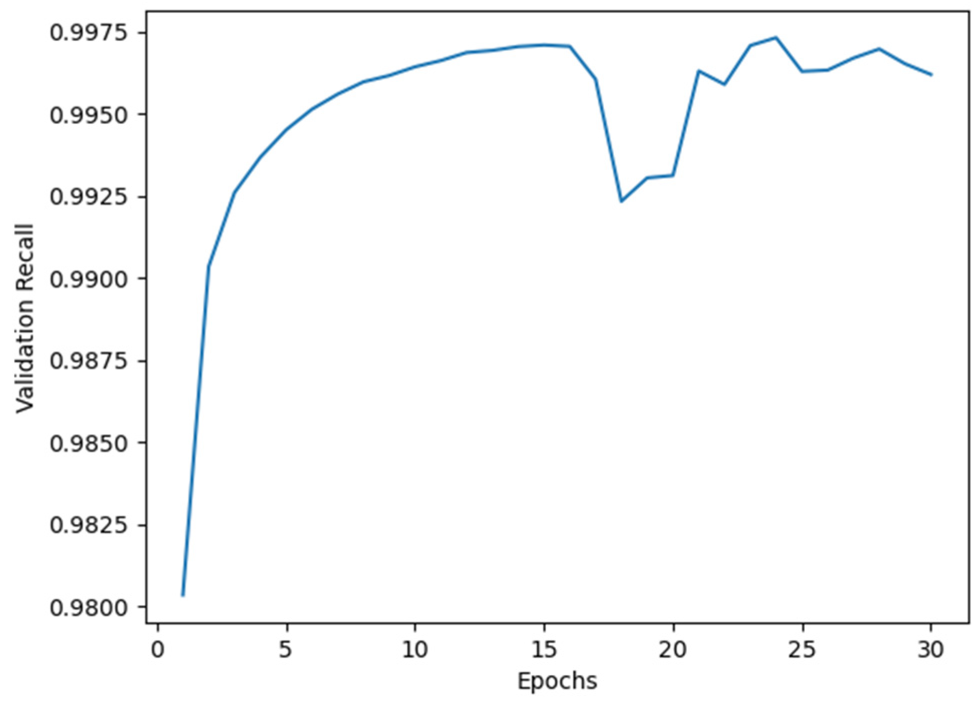
For Model I, the average accuracy and recall values obtained from cross-validation are illustrated in Figure 2 and Figure 3, respectively. As shown in these figures, a dip suggesting potential overfitting appeared around the 16th epoch. However, as our primary goal in this security-critical domain is minimizing false negatives, we prioritized maximizing the Recall metric. Although validation recall showed volatility after epoch 16 (as shown in Figure 4), it subsequently recovered and reached its peak value at epoch 24. We therefore selected 24 as the optimal training epoch for Model I.

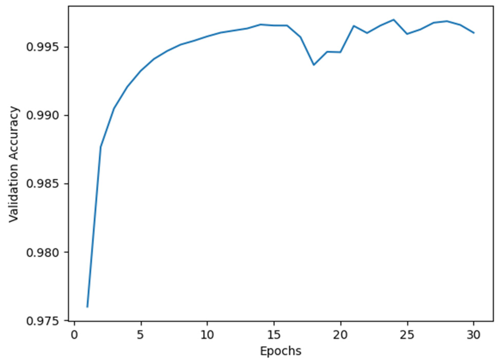
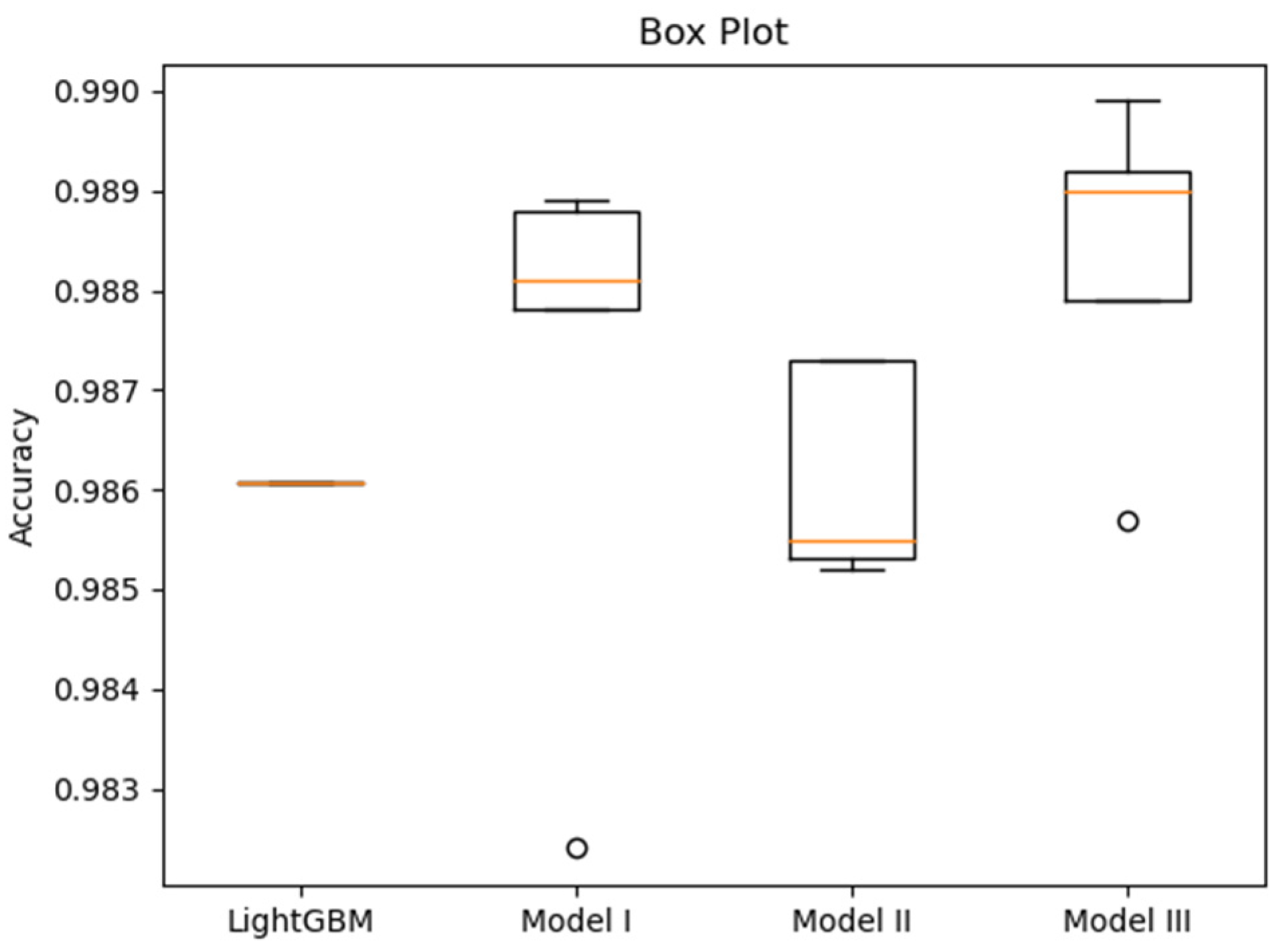
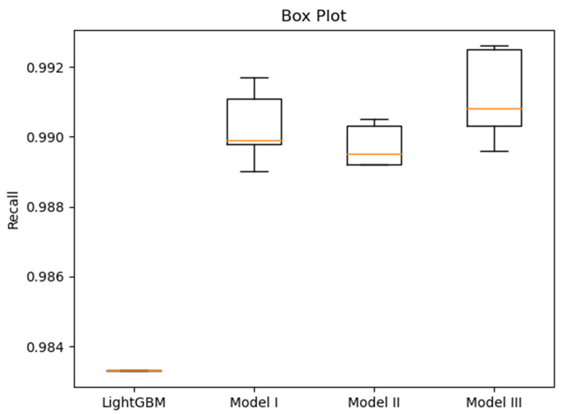
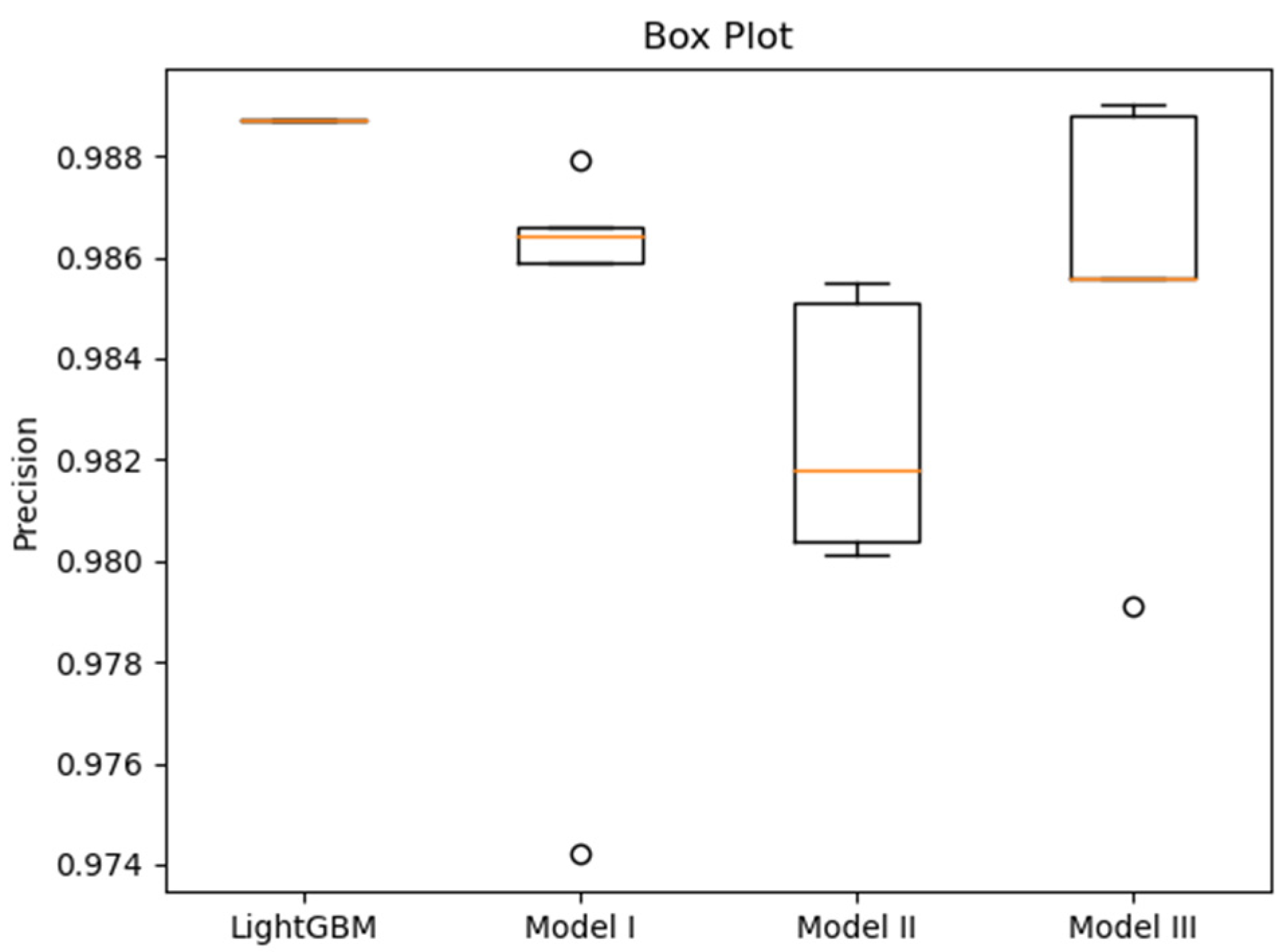
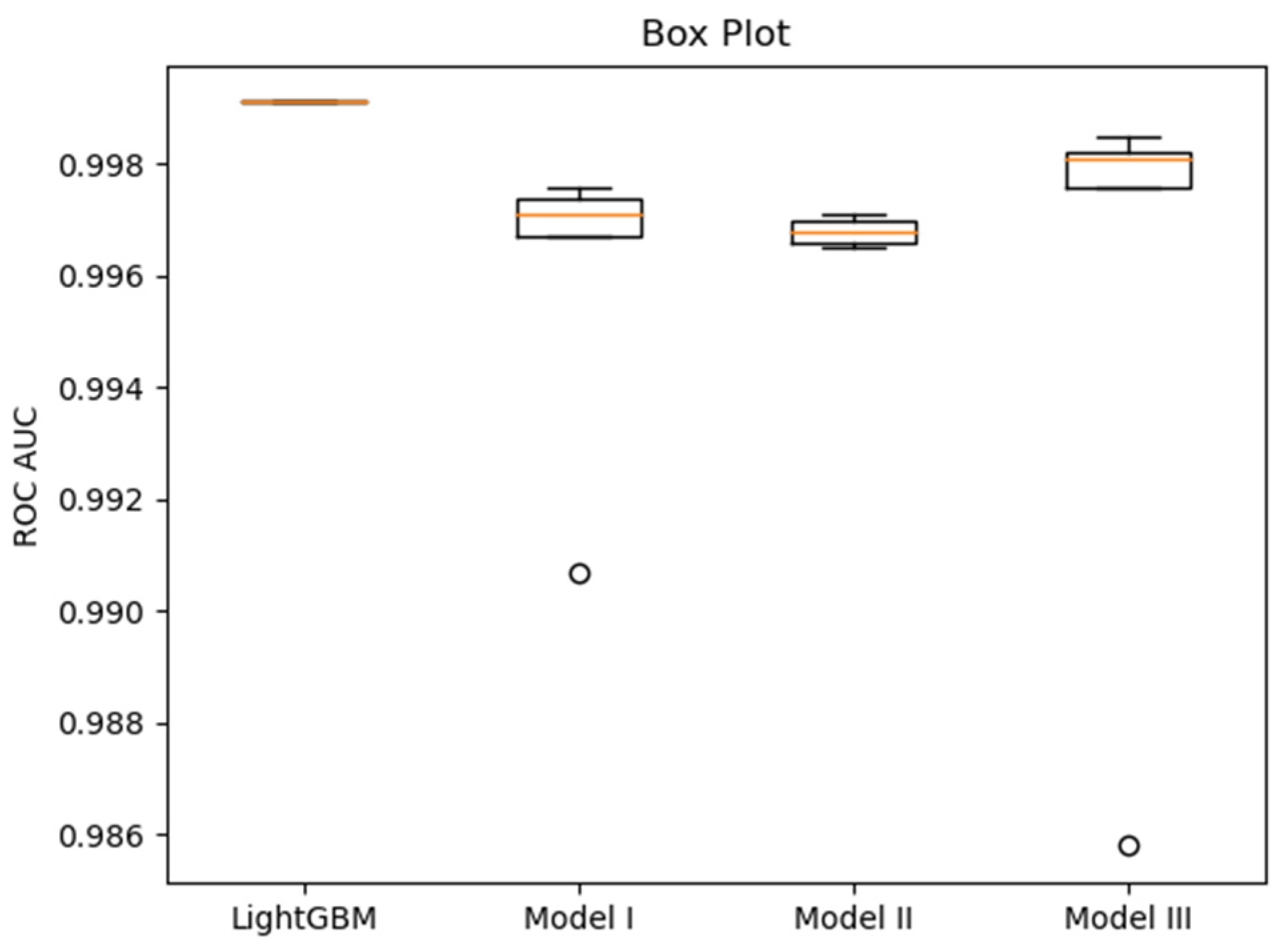
Following the same procedure, cross-validation identified 24 as the optimal epoch for Model II and 30 for Model III (see Appendix A, Figure A4, Figure A5, Figure A6 and Figure A7), providing the basis for subsequent performance comparison. To visually compare the performance variability of the models based on the fivefold cross-validation, box plots for accuracy, recall, precision, and ROC AUC are presented in Figure 4, Figure 5, Figure 6 and Figure 7, respectively. These plots visualize the median, interquartile range (IQR), and outliers from the five folds, providing a more comprehensive view of model stability than mean values alone. To enable a direct comparison with prior work, we additionally implemented the LightGBM model proposed by Anderson et al. [16] and the deep learning model presented by Sumit et al. [17], both trained and validated under identical experimental conditions.

After analyzing the individual models and their validation distributions, we consolidated the performance metrics for comparison.

Table 5. Performance comparison of machine learning and deep learning models on the EMBER dataset. Metrics for Models I, II, and III are shown as the Mean ± Standard Deviation from fivefold cross-validation.

Model	Training Time (s)	Accuracy	Precision	Recall	F1	ROC AUC
LightGBM [16]	840	0.9861	0.9888	0.9833	0.9860	0.9991
Sumit et al. [17]	130	0.9541	0.9819	0.9253	0.9528	0.9913
Model I	326	0.9872 ± 0.0027	0.9842 ± 0.0056	0.9903 ± 0.0011	0.9872 ± 0.0026	0.9959 ± 0.0029
Model II	326	0.9861 ± 0.0011	0.9826 ± 0.0026	0.9897 ± 0.0006	0.9861 ± 0.0011	0.9968 ± 0.0003
Model III	845	0.9883 ± 0.0016	0.9857 ± 0.0040	0.9912 ± 0.0013	0.9884 ± 0.0016	0.9956 ± 0.0055

Note: Bold numbers denote the best performance in each metric.

summarizes the fivefold cross-validation (Mean ± SD) results for all proposed models against the baselines. Several key observations can be drawn:

• LightGBM achieved the highest ROC AUC and Precision.
• All three proposed deep neural network models obtained higher Recall than LightGBM, albeit with lower Precision. This indicates that the DNNs generated fewer false negatives (malicious files misclassified as benign) but more false positives compared with LightGBM. In practical terms, the proposed models reduce the risk of undetected malware.
• Recall is particularly critical in malware classification as it reflects the ability to correctly identify malicious samples and avoid false negatives. Among the models, Model III achieved the highest Recall.
• Model II achieved the highest ROC AUC among the deep neural networks. Model III, with a training time comparable to LightGBM, nevertheless outperformed LightGBM in terms of Accuracy, Recall, and F1 Score.

Together, these findings demonstrate that while LightGBM remains strong in terms of precision-oriented metrics, the proposed deep learning models—especially Model III—offer superior recall and balanced performance, which are particularly valuable in security-critical applications.

4.3. Effect of Feature Selection

4.3.1. Feature Reduction Based on Kumar et al.’s 276 Selected Features

Given the need to reduce feature dimensionality, we examined whether the feature vectors in the EMBER dataset could be effectively streamlined. To this end, we adopted the 276 features proposed by Kumar et al. [14] and applied them to the three deep learning models developed in this study. After reducing the input dimensionality to 276, the dense layers of each model were proportionally scaled down. The resulting hidden units were set to 180, 150, 120, 90, 60, and 30, respectively.

The results in

Table 6. Performance using the 276 selected features proposed by Kumar et al. [14]. Metrics are shown as the Mean ± Standard Deviation from fivefold cross-validation.

Model	Total Parameters	Training Time (s)	Accuracy	Precision	Recall	F1	ROC AUC
Model I	113,341	293	0.9811 ± 0.0017	0.9733 ± 0.0044	0.9895 ± 0.0012	0.9813 ± 0.0017	0.9973 ± 0.0005
Model II	113,341	293	0.9783 ± 0.0043	0.9710 ± 0.0063	0.9862 ± 0.0026	0.9785 ± 0.0042	0.9972 ± 0.0007
Model III	115,861	837	0.9842 ± 0.0016	0.9801 ± 0.0031	0.9886 ± 0.0010	0.9843 ± 0.0016	0.9975 ± 0.0007

Note: Bold numbers denote the best performance in each metric.

demonstrate that the use of Kumar et al.’s selected features enabled the construction of models with competitive performance while substantially reducing the number of parameters. Notably, Model III achieved superior performance across nearly all evaluation metrics compared with Models I and II, except for recall and training time, where its performance was less favorable.

These findings confirm that Kumar’s feature selection method provides an effective means of reducing model complexity without sacrificing accuracy. The next subsection further investigates an alternative reduction strategy based on LightGBM feature importance.

4.3.2. Feature Reduction via 206 Intersection Features Obtained from the LightGBM Model

Building on the methodology of Kumar et al. [14], we investigated an alternative approach for feature reduction. The LightGBM model provides a Feature Importance function that ranks features using two complementary criteria: Information Gain, which reflects how much a feature contributes to classification decisions, and Weight, which indicates how frequently a feature is used during training. Using this function, we first identified the top 276 features ranked by Information Gain and another 276 ranked by Weight. By intersecting the two sets, we obtained 206 shared features, which were then used to train the three proposed models. The corresponding validation metrics are presented in

Table 7. Performance using the 206 intersection features obtained from the LightGBM model. Metrics are shown as the Mean ± Standard Deviation from fivefold cross-validation.

Model	Total Parameters	Accuracy	Precision	Recall	F1	ROC AUC
Model I	100,741	0.9753 ± 0.0022	0.9649 ± 0.0047	0.9865 ± 0.0019	0.9756 ± 0.0021	0.9938 ± 0.0006
Model II	100,741	0.9771 ± 0.0034	0.9731 ± 0.0065	0.9813 ± 0.0032	0.9772 ± 0.0033	0.9965 ± 0.0009
Model III	103,261	0.9815 ± 0.0024	0.9770 ± 0.0053	0.9863 ± 0.0029	0.9816 ± 0.0023	0.9974 ± 0.0009

Note: Bold numbers denote the best performance in each metric.

.

The results are significant. With only 206 features, the models retained performance levels comparable to those trained with 276 features or even the full set of 2351. Model III achieved an accuracy of 98.15% and an AUC of 0.9974. Apart from recall—where its improvement was less pronounced, Model III outperformed Models I and II across all other metrics. These findings demonstrate that substantial dimensionality reduction can be achieved without compromising the classification quality, thereby reinforcing the effectiveness of embedding feature reduction into the preprocessing pipeline.

4.4. Generalization Assessment via Cross-Dataset Validation

To evaluate the generalization capability of our models beyond EMBER, we conducted cross-dataset validation using the publicly available REWEMA dataset [12]. In this experiment, the models trained on EMBER, as described in Section 4.2, were directly tested on REWEMA, and their performance metrics are summarized in

Table 8. Performance of Models I–III and LightGBM under cross-dataset validation using REWEMA. Metrics for Models I, II, and III are shown as the Mean ± Standard Deviation from fivefold cross-validation.

Model	Accuracy	Precision	Recall	F1	ROC AUC
LightGBM [16]	0.7822	0.9201	0.6157	0.7377	0.8559
Model I	0.7626 ± 0.0196	0.8788 ± 0.0349	0.6075 ± 0.0327	0.7177 ± 0.0259	0.8350 ± 0.0184
Model II	0.7688 ± 0.0160	0.9018 ± 0.0051	0.6008 ± 0.0361	0.7206 ± 0.0260	0.8398 ± 0.0179
Model III	0.7787 ± 0.0105	0.9248 ± 0.0098	0.6043 ± 0.0194	0.7308 ± 0.0154	0.8467 ± 0.0190

Note: Bold numbers denote the best performance in each metric.

.

The cross-dataset validation on REWEMA yielded several key insights (Table 8). First, Model III maintained the best overall performance among the proposed DNNs, leading in Accuracy, Precision, F1-score, and ROC AUC. More importantly, when compared to the LightGBM baseline, a notable finding emerged. Although performance dropped across all models, which reflects the known challenge of dataset distribution shift, Model III achieved a higher Precision (0.9248) than LightGBM (0.9201). While LightGBM maintained an advantage in overall Accuracy and Recall, Model III’s superior precision on an independent dataset suggests a greater resilience against false positives when faced with new, unseen data, highlighting the potential of its architecture.

5. Discussion

This study systematically evaluated three deep neural network architectures for static malware classification and compared them against the LightGBM baseline using publicly available datasets. LightGBM achieved superior precision and ROC AUC, whereas the proposed Model III consistently delivered the best accuracy, recall, and F1-score. Notably, its recall exceeded that of LightGBM by 0.73%, underscoring its strength in reducing false negatives—an especially critical property in security-sensitive applications.

We acknowledge that various SOTA models exist beyond our primary baselines. For instance, as noted in Section 2, Pramanik et al. [18] explored CNNs on this same dataset, finding their fully connected model to be superior. Our study’s primary objective, however, was to optimize DNN performance against the established and highly potent LightGBM baseline provided by the EMBER dataset’s authors [16]. As shown in our own results (Table 5) and the original EMBER paper [16], the LightGBM baseline already achieved a near-perfect ROC AUC of 0.9991. On such a saturated benchmark, it is notoriously difficult for more complex models—including the CNNs tested by Pramanik et al. [18]—to demonstrate a significant overall advantage. Therefore, our contribution lies not in outperforming all possible SOTA architectures, but in demonstrating that through specific architectural optimization (Model III), we can achieve a targeted, significant improvement in the critical metric of Recall (a 0.73% increase over LightGBM). We argue that this is a valuable finding for minimizing false negatives, even on a benchmark where the overall accuracy metrics are already near-perfect.

In the feature selection experiments, both the Kumar method (276 features) and the LightGBM-based intersection method (206 features) substantially reduced the training time while maintaining high classification accuracy. Between the two, the Kumar method provided a better balance between performance retention and computational efficiency. This result highlights that dimensionality reduction is not merely a computational convenience, but a strategic design choice that can enhance deployment in resource-constrained or rapid-response environments.

Cross-dataset validation using REWEMA revealed a performance decline across all models (Table 8). A potential concern is that our epoch selection (e.g., 24 for Model I, 30 for Model III) prioritized peak Recall over the absolute lowest validation loss, which could risk generalization. This was a deliberate trade-off, as our cross-validation curves (Figure 3, Figure A5 and Figure A7) demonstrate these later epochs achieved the highest Recall, a critical metric for minimizing false negatives. However, we attribute the significant drop primarily to dataset distribution shift. As noted in Section 4.4, the malicious samples in REWEMA originate from different sources and families than those in EMBER. This heterogeneity is a known generalization challenge. Nevertheless, the reduction observed in the DNN models was less pronounced than that of LightGBM, indicating stronger adaptability. Model III maintained leading F1-scores, further validating the robustness of its architecture and suggesting that deep models hold promise for real-world malware detection.

Several limitations should also be acknowledged. First, our study used the EMBER 2017 (v1) dataset to maintain methodological consistency with the foundational literature [16,17] used for our baseline comparisons. We acknowledge that the EMBER 2018 (v2) dataset addresses potential label noise, and validating our architectures on this and newer benchmarks remains a critical direction for future work. Second, the study focused exclusively on Windows PE-format datasets, thereby excluding other operating systems and file types. Moreover, model performance remains closely tied to specific feature extraction and engineering strategies, and the semantic relationship between selected features and malicious behavior patterns was not fully explored. Future research should address these gaps by integrating multimodal features, extending evaluation to cross-platform datasets, adopting interpretable model designs, and developing resource-efficient real-time deployment strategies. In particular, explainable AI techniques could help translate feature importance into actionable insights for malware analysts, thereby bridging the gap between algorithmic predictions and practical security operations.

6. Conclusions

This study proposed and evaluated three deep neural network (DNN) architectures for static malware classification, benchmarked against the LightGBM baseline using the EMBER and REWEMA datasets. Experimental results demonstrated that while LightGBM achieved superior precision and ROC AUC, the proposed Model III consistently delivered the best accuracy, recall, and F1-score. Its 0.73% improvement in recall over LightGBM is particularly noteworthy, as it highlights the model’s ability to reduce false negatives—a critical requirement in security-sensitive environments.

Feature selection experiments further revealed the value of dimensionality reduction. Both the Kumar method (276 features) and the LightGBM-based intersection method (206 features) significantly reduced the training time while maintaining competitive accuracy. Among these, the Kumar method provided the most favorable balance between performance retention and efficiency, underscoring the practical role of feature reduction in real-world deployment scenarios.

Cross-dataset validation using REWEMA confirmed the robustness of the proposed models while also revealing their sensitivity to distributional shifts. Although performance declined compared with EMBER, the degradation observed in the DNNs was less pronounced than that of LightGBM, demonstrating stronger adaptability to heterogeneous data. Model III, in particular, maintained leading F1-scores, reinforcing the resilience of its design.

Taken together, these findings highlight that architectural optimization combined with informed feature selection can substantially enhance static malware classification. Future research should expand this line of work by incorporating multimodal features, extending validation to cross-platform datasets, and developing interpretable and resource-efficient deep learning models. In particular, explainable AI techniques represent a promising direction to translate feature importance into actionable insights, thereby bridging the gap between algorithmic predictions and practical cybersecurity operations.

References

- Aslan, O.; Samet, R. A Comprehensive Review on Malware Detection Approaches. IEEE Access 2020, 8, 6249–6271. [Google Scholar] [CrossRef]
- Caviglione, L.; Choraś, M.; Corona, I.; Janicki, A.; Mazurczyk, W.; Pawlicki, M.; Wasielewska, K. Tight Arms Race: Overview of Current Malware Threats and Trends in Their Detection. IEEE Access 2021, 9, 5371–5396. [Google Scholar] [CrossRef]
- Gibert, D.; Mateu, C.; Planes, J. The Rise of Machine Learning for Detection and Classification of Malware: Research Developments, Trends and Challenges. J. Netw. Comput. Appl. 2020, 153, 102526. [Google Scholar] [CrossRef]
- Zatloukal, F.; Znoj, J. Malware Detection Based on Multiple PE Headers Identification and Optimization for Specific Types of Files. J. Adv. Eng. Comput. 2017, 1, 153. [Google Scholar] [CrossRef]
- Wang, T.-Y.; Wu, C.-H.; Hsieh, C.-C. Detecting Unknown Malicious Executables Using Portable Executable Headers. In Proceedings of the 2009 Fifth International Joint Conference on INC, IMS and IDC, Seoul, Republic of Korea, 25–27 August 2009; pp. 278–284. [Google Scholar]
- Rezaei, T.; Hamze, A. An Efficient Approach For Malware Detection Using PE Header Specifications. In Proceedings of the 2020 6th International Conference on Web Research (ICWR), Tehran, Iran, 22–23 April 2020; IEEE: New York, NY, USA, 2020; pp. 234–239. [Google Scholar]
- Microsoft Windows Portable Excutable. Available online: https://learn.microsoft.com/en-us/windows/win32/debug/pe-format (accessed on 11 September 2025).
- Ahmadi, M.; Ulyanov, D.; Semenov, S.; Trofimov, M.; Giacinto, G. Novel Feature Extraction, Selection and Fusion for Effective Malware Family Classification. In Proceedings of the Sixth ACM Conference on Data and Application Security and Privacy, New Orleans, LA, USA, 9–11 March 2016; ACM: Nashville, Tennessee, 2016; pp. 183–194. [Google Scholar]
- Rezaei, T.; Manavi, F.; Hamzeh, A. A PE Header-Based Method for Malware Detection Using Clustering and Deep Embedding Techniques. J. Inf. Secur. Appl. 2021, 60, 102876. [Google Scholar] [CrossRef]
- Raff, E.; Sylvester, J.; Nicholas, C. Learning the PE Header, Malware Detection with Minimal Domain Knowledge. In Proceedings of the 10th ACM Workshop on Artificial Intelligence and Security, Dallas, TX, USA, 3 November 2017; ACM: Nashville, Tennessee, 2017; pp. 121–132. [Google Scholar]
- EMBER. Elastic Malware Benchmark for Empowering Researchers. Available online: https://github.com/elastic/EMBER (accessed on 11 September 2025).
- REWEMA. Retrieval Windows Executables Malware Analysis. Available online: https://github.com/rewema/REWEMA (accessed on 11 September 2025).
- Oyama, Y.; Miyashita, T.; Kokubo, H. Identifying Useful Features for Malware Detection in the Ember Dataset. In Proceedings of the 2019 Seventh International Symposium on Computing and Networking Workshops (CANDARW), Nagasaki, Japan, 26–29 January 2019; pp. 360–366. [Google Scholar]
- Kumar, R. Malware Classification Using XGboost-Gradient Boosted Decision Tree. Adv. Sci. Technol. Eng. Syst. J. 2020, 5, 536–549. [Google Scholar] [CrossRef]
- Pham, H.-D.; Le, T.D.; Vu, T.N. Static PE Malware Detection Using Gradient Boosting Decision Trees Algorithm. In Future Data and Security Engineering; Dang, T.K., Küng, J., Wagner, R., Thoai, N., Takizawa, M., Eds.; Lecture Notes in Computer Science; Springer International Publishing: Cham, Switzerland, 2018; Volume 11251, pp. 228–236. ISBN 978-3-030-03191-6. [Google Scholar]
- Anderson, H.S.; Roth, P. EMBER: An Open Dataset for Training Static PE Malware Machine Learning Models. arXiv 2018, arXiv:1804.04637. [Google Scholar] [CrossRef]
- Lad, S.S.; Adamuthe, A.C. Improved Deep Learning Model for Static PE Files Malware Detection and Classification. IJCNIS 2022, 14, 14–26. [Google Scholar] [CrossRef]
- Pramanik, S.; Teja, H. EMBER—Analysis of Malware Dataset Using Convolutional Neural Networks. In Proceedings of the 2019 Third International Conference on Inventive Systems and Control (ICISC), Coimbatore, India, 10–11 January 2019; pp. 286–291. [Google Scholar]
- Ronen, R.; Radu, M.; Feuerstein, C.; Yom-Tov, E.; Ahmadi, M. Microsoft Malware Classification Challenge. arXiv 2018, arXiv:1802.10135. [Google Scholar] [CrossRef]
- LIEF. Library to Instrument Executable Formats. Available online: https://github.com/lief-project/LIEF (accessed on 11 September 2025).
- Hex-Rays IDA. Available online: https://www.hex-rays.com/ida-pro/ (accessed on 11 September 2025).
- Weinberger, K.; Dasgupta, A.; Langford, J.; Smola, A.; Attenberg, J. Feature Hashing for Large Scale Multitask Learning. In Proceedings of the 26th Annual International Conference on Machine Learning, New York, NY, USA, 14–18 June 2009; Association for Computing Machinery: New York, NY, USA, 2009; pp. 1113–1120. [Google Scholar]
- de Boer, P.-T.; Kroese, D.P.; Mannor, S.; Rubinstein, R.Y. A Tutorial on the Cross-Entropy Method. Ann. Oper. Res. 2005, 134, 19–67. [Google Scholar] [CrossRef]
- Vinayakumar, R.; Soman, K.P. DeepMalNet: Evaluating Shallow and Deep Networks for Static PE Malware Detection. ICT Express 2018, 4, 255–258. [Google Scholar] [CrossRef]
- Ramachandran, P.; Zoph, B.; Le, Q.V. Searching for Activation Functions. arXiv 2017, arXiv:1710.05941. [Google Scholar] [CrossRef]
- Kingma, D.P.; Ba, J. Adam: A Method for Stochastic Optimization. arXiv 2017, arXiv:1412.6980. [Google Scholar] [CrossRef]
- Tharwat, A. Classification Assessment Methods. Appl. Comput. Inform. 2020, 17, 168–192. [Google Scholar] [CrossRef]