A Classified Branch–CapNet: A Multi-Modal Model with Classified Branches for the Capacity Prediction of Li–Ion Battery Cathodes

Abstract

Machine learning has emerged as a promising tool to accelerate the screening of lithium–ion battery electrode materials. Gravimetric capacity, a critical performance indicator governing electrode energy density, is intrinsically related to lithium insertion and extraction mechanisms, requiring sophisticated embedding approaches that capture the structural characteristics of cathode materials. The cathode material dataset from the Materials Project database comprises heterogeneous data modalities: numerical features representing chemical properties and categorical features encoding structural characteristics. Naive integration of these disparate data types may introduce semantic gaps from statistical distributional discrepancies, potentially degrading predictive performance and limiting model generalization. To address these limitations, this study proposes a Classified Branch–CapNet model that individually embeds four distinct types of categorical structural data into separate classified branches along with numerical data for independent learning, subsequently integrating them through a late fusion strategy. This approach minimizes interference between heterogeneous data modalities while capturing structure–property relationships with enhanced precision. The proposed model achieved superior performance with a mean absolute error of 2.441 mAh/g, demonstrating substantial improvements of 56.2%, 71.2%, 73.9%, and 51.1% over conventional deep neural networks, recurrent neural networks, long short-term memory architectures, and the encoder-only Transformer, respectively. Furthermore, it achieved the lowest root mean square error of 15.236 mAh/g and the highest coefficient of determination of 0.961, confirming its superior predictive accuracy and generalization capability compared with all benchmark models. Our model therefore demonstrates significant potential to accelerate the efficient screening and discovery of high-performance battery electrode materials.

1. Introduction

The need for high-performance energy storage technologies has become increasingly important across various applications, which include electric vehicles (EVs), smart grids, and renewable energy systems. Lithium–ion batteries (LIBs) are currently the most widely adopted battery technology, primarily due to their high energy density and long-life cycle [1]. However, current LIB technologies face limitations in meeting the rapidly increasing demands for greater energy storage capacity and enhanced performance. Many conventional electrode materials are already reaching the ceiling of their theoretical capacities, while practical issues, such as high production costs, unstable material supply, and increasing demand for longer cycle life and higher performance, remain unresolved [2]. To address these challenges, the development of high-capacity electrode materials that can overcome the limitations of conventional materials is essential [3]. Gravimetric capacity refers to the amount of charge that can be stored or delivered per unit mass of the active material and is intimately correlated with practical driving range, energy density, and cycle life. Consequently, the development of high-capacity cathode materials is regarded as a pivotal design objective to enhance the competitiveness of EVs and next-generation energy storage systems. A range of cathode materials with various crystal structures has been actively investigated to achieve this objective. Representative examples include layered structures LiCoO₂, LiNiO₂, and ternary NCM compounds LiNi_1−x−yCo_xMn_yO₂, as well as spinel-type LiMn₂O₄ and olivine-type LiFePO₄. These diverse cathode chemistries provide advantages in terms of structural stability and ionic conductivity, which collectively enhance the overall performance of LIBs [4,5,6]. However, the conventional trial-and-error approach to discovering new electrode materials remains time-consuming and resource-intensive, thereby impeding the ability to keep pace with the rapidly increasing demand. To address this limitation, Density Functional Theory (DFT)-based computational methods have been employed to predict material properties [7]. While DFT offers invaluable insights into chemical structure and stability, it often requires computation times that range from several to hundreds of hours, posing a significant bottleneck for the high-throughput screening of candidate materials. Recently, the construction of large-scale computational materials databases—including the Materials Project, The Open Quantum Materials Database (OQMD), The Novel Materials Discovery (NOMAD), and Automatic Flow (AFLOW)—has enabled machine learning (ML) methodologies to fundamentally revolutionize the paradigm of materials discovery [8,9,10,11,12]. Machine learning enables rapid property prediction by effectively capturing the complex and nonlinear relationships among diverse input features that include chemical composition, crystal structure, and electronic properties [13]. Manna et al. designed leveraged structural and elemental property datasets of Li, Na, and K–ion electrode materials collected from the Materials Project database to develop machine learning models that were capable of predicting the capacity of unknown K–ion electrode materials. This computational approach demonstrated that ML-based methodologies can effectively screen electrode materials with significantly reduced computational expense, compared to quantum mechanical calculations [14]. Zhang et al. enhanced the accuracy of their machine learning models to predict electrode voltage and capacity by applying a sequential backward selection (SBS) method to determine the optimal feature set. Furthermore, through Shapley additive explanations (SHAP)-based interpretability analysis, they quantified how different categories of features contribute to model outputs, thereby yielding actionable insights to guide future studies in data-driven electrode design [15]. Ma et al. developed two types of models—one that rapidly predicts electrochemical properties using a simple set of input features, and another high-precision model leveraging a complete set of complex features for the deep mining of current datasets with significantly improved accuracy. These models, capable of simultaneously predicting average voltage, specific capacity, and specific energy, contributed to the accelerated screening and design of next-generation high-performance battery materials [16]. Zhou et al. employed a crystal graph convolutional neural network (CGCNN)-based deep learning model to screen approximately 130,000 inorganic compounds and identified candidate Zn cathode materials with high voltage and high capacity, thereby contributing to the discovery of reliable cathode materials. By integrating potential data from the Materials Project (MP) and AFLOW databases, they enhanced predictive accuracy and alignment with experimental results, ultimately expanding the application potential of Zn batteries, which had been limited by a lack of suitable cathode materials [17]. Wang et al. developed a modified version of the CGCNN deep-learning framework that successfully merges structural characteristics with the physicochemical properties of materials. By overcoming the data-fusion limitations of prior approaches, this model markedly improves both the efficiency and predictive accuracy of gravimetric capacity estimation in lithium–ion batteries [18].

While these studies demonstrate the considerable potential of ML-based approaches for battery material capacity prediction, several critical limitations still remain. First, existing approaches to embedding the structural data of cathode materials frequently fail to reflect the underlying physical significance inherent in the material’s structure. In many studies, structural data are embedded using simplistic methods that inadequately capture the intricate geometric and topological features of crystal structures. Consequently, these reductive approaches can obscure or distort the fundamental structure–property relationships between crystallographic architecture and electrochemical capacity during the feature transformation process, thereby limiting the predictive accuracy and physical interpretability of the ML models. Second, the Crystal Graph Convolutional Neural Network (CGCNN), a universal and interpretable framework for crystalline materials, effectively captures local chemical semantics by learning atomic interactions and bonding relationships through graph representations. However, it has limitations in capturing global periodic structural information, such as crystallographic symmetry, which significantly influences macroscopic material properties. This deficiency in representing the characteristic of crystal structures can compromise the model’s ability to fully exploit structure–property relationships for precise gravimetric capacity estimation in battery materials [19]. Furthermore, although capacity-determining factors extend beyond composition to include variables such as the crystal system and ion types, employing CGCNN alone to encode structural information may prove insufficient to accurately elucidate the complex structure–property correlations [20,21,22]. Third, conventional approaches naively integrate categorical and numerical features, which possess distinct statistical properties, into a single input vector, thereby inducing a semantic gap due to this statistical mismatch. In particular, categorical structural data tend to be sparse, whereas numerical data exhibit dense distributions, making joint learning challenging and unlikely to ensure reliable performance [23]. In this context, it has been reported that the integration of heterogeneous multi-modal data can degrade model performance during training, owing to the inherent disparity in data modalities [24]. Notably, conventional late fusion approaches integrate branch outputs through simple weighted averaging, with uniform weighting assigned to all modalities regardless of their information density [25]. This simplistic integration strategy fails to reflect the heterogeneous information content across modalities, treating features with high information density identically to those with lower information density. For instance, chemical composition typically contains greater information density regarding gravimetric capacity prediction compared to structural embeddings; however, conventional late fusion assigns identical weights to both modalities. Consequently, compositionally critical information may be insufficiently learned, compromising prediction reliability and model generalization. Furthermore, existing multi-modal architectures remain vulnerable to noise contamination in heterogeneous feature representations, wherein noise in one modality can adversely affect the integrated prediction [26]. Collectively, these limitations represent a critical yet unaddressed research gap: despite advances in individual embedding techniques and feature integration methods, no unified framework exists that simultaneously tackles the physical interpretability of structural embeddings, the global structural encoding limitations of graph-based approaches, and the statistical heterogeneity inherent in categorical-numerical feature fusion. This gap is particularly pronounced in Materials Project-based screening, where categorical embeddings (sparse) and numerical properties (dense) exhibit fundamentally different statistical characteristics requiring strategically differentiated treatment. To overcome the limitations of existing approaches, this work proposes a three-stage model design strategy, leveraging lithium–ion cathode data from the Materials Project database, which comprises (1) embedding physically meaningful structural representations, (2) alleviating sparsity through feature extraction based on effective dimensionality reduction method, and (3) enabling modality-independent learning across heterogeneous data sources. Specifically, we first design individual embeddings for four items of structural information—formula, crystal system, general formula, and ion type—grounded in their structural semantics, then apply non-negative matrix factorization (NMF) for dimensionality reduction to alleviate feature sparsity [27]. Subsequently, within a multi-branch deep neural network employing a late-fusion architecture, numerical chemical features (e.g., band gap, stability, Fermi level) and structural features are learned through separate network branches, and their resulting feature representations are then integrated to minimize the semantic gap. By overcoming the limitations of existing single-path learning and naively integrated feature representations, the proposed model independently optimizes categorical and numerical data through optimized pathways, effectively bridging the semantic gap and enabling more accurate gravimetric capacity prediction. Moreover, its design strategy establishes a crucial paradigm for the AI-driven screening of high-capacity cathode materials by minimizing data heterogeneity and exquisitely capturing structure–property correlations to maximize predictive performance.

2. Data Embedding Methodology and Stochastic Analysis

In this study, lithium–ion battery cathode material data were acquired from the MP database [8]. The MP database encompasses property information for thousands of electrode materials in both lithium intercalated and deintercalated states obtained through DFT-based high-throughput calculations, hence providing a comprehensive data source for materials property prediction. Data collection was performed using the MP application programming interface (MP–API), followed by systematic preprocessing to eliminate missing values, ultimately yielding a curated dataset comprising 2424 lithium–ion cathode materials. The dataset includes four categories of features: stoichiometric properties (Formula, General Formula), structural properties (Crystal System), electronic properties (Band Gap, Fermi Level), and electrochemical properties (Ion Type, Stability). As detailed in

Table 1. Input feature classification employed in this study, derived from the Materials Project database.

Data Type	Feature Name	Description
Categorical	Formula	Chemical composition
	Crystal System	Set of point groups
	General Formula	Generalized composition pattern
	Ion Type	Element list
Numerical	Band Gap	Valence–conduction gap
	Stability	Thermodynamic stability
	Fermi Level	Thermodynamic electron- energy

, these features encompass both categorical and numerical modalities. Importantly, the MP dataset exhibits certain characteristics that warrant explicit discussion: (1) Structural bias—the dataset is non-uniformly distributed across crystal systems, with certain structures overrepresented, potentially biasing model predictions toward prevalent structural families; (2) Environmental bias—the data comprises computationally predicted properties under ideal conditions, not accounting for actual synthesis feasibility or experimental battery operating conditions. To address these biases, we employed stratified sampling across crystal systems during data partitioning. These considerations should inform the interpretation of model predictions in practical applications. The primary objective of the predictive model is to accurately forecast the gravimetric capacity (mAh/g) based on the corresponding input features. To achieve this goal, two distinct feature modalities—categorical and numerical—were strategically selected from the MP database, as summarized in Table 1:

The strategic design of input features in deep learning-based materials property prediction models constitutes a pivotal component of the computational framework. In the present investigation, the embedding architecture was deliberately differentiated with particular emphasis on preserving the structural meaning of categorical features. Although previous studies have employed conventional Principal Component Analysis (PCA) for categorical feature processing [15], standard PCA demonstrates intrinsic limitations whereby structural information characterized by inherent sparsity may be compromised [28]. Accordingly, in this work, Non-negative Matrix Factorization (NMF) was adopted as the feature extraction algorithm owing to its demonstrated superior capability in capturing and preserving the sparsity characteristics inherent in string-based embedding data [27].

2.1. Formula Embedding

The chemical formula encodes elemental composition and stoichiometric information, which directly affects theoretical lithium–ion insertion capacity. In this work, fixed elemental indices were established based on the MP dataset, and atomic counts were encoded at corresponding index positions to create numerical feature vectors suitable for machine learning. This approach captures the underlying physical relationship between composition and capacity, offering advantages over conventional one-hot encoding schemes.

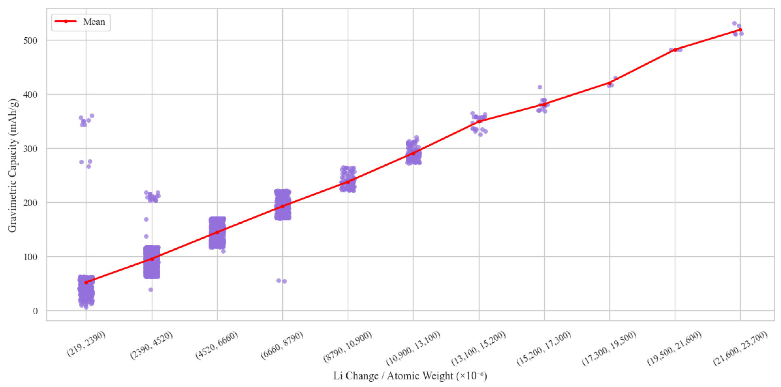
Figure 1 shows that while gravimetric capacity generally increases with higher lithium-to-molecular-weight ratios, considerable variations exist within identical ratio intervals, indicating that compositional ratios alone cannot fully explain capacity variations. These variations suggest that structural characteristics, such as crystal system, significantly influence capacity performance. Therefore, structural information was also embedded and incorporated into the learning framework.

2.2. Crystal System Embedding

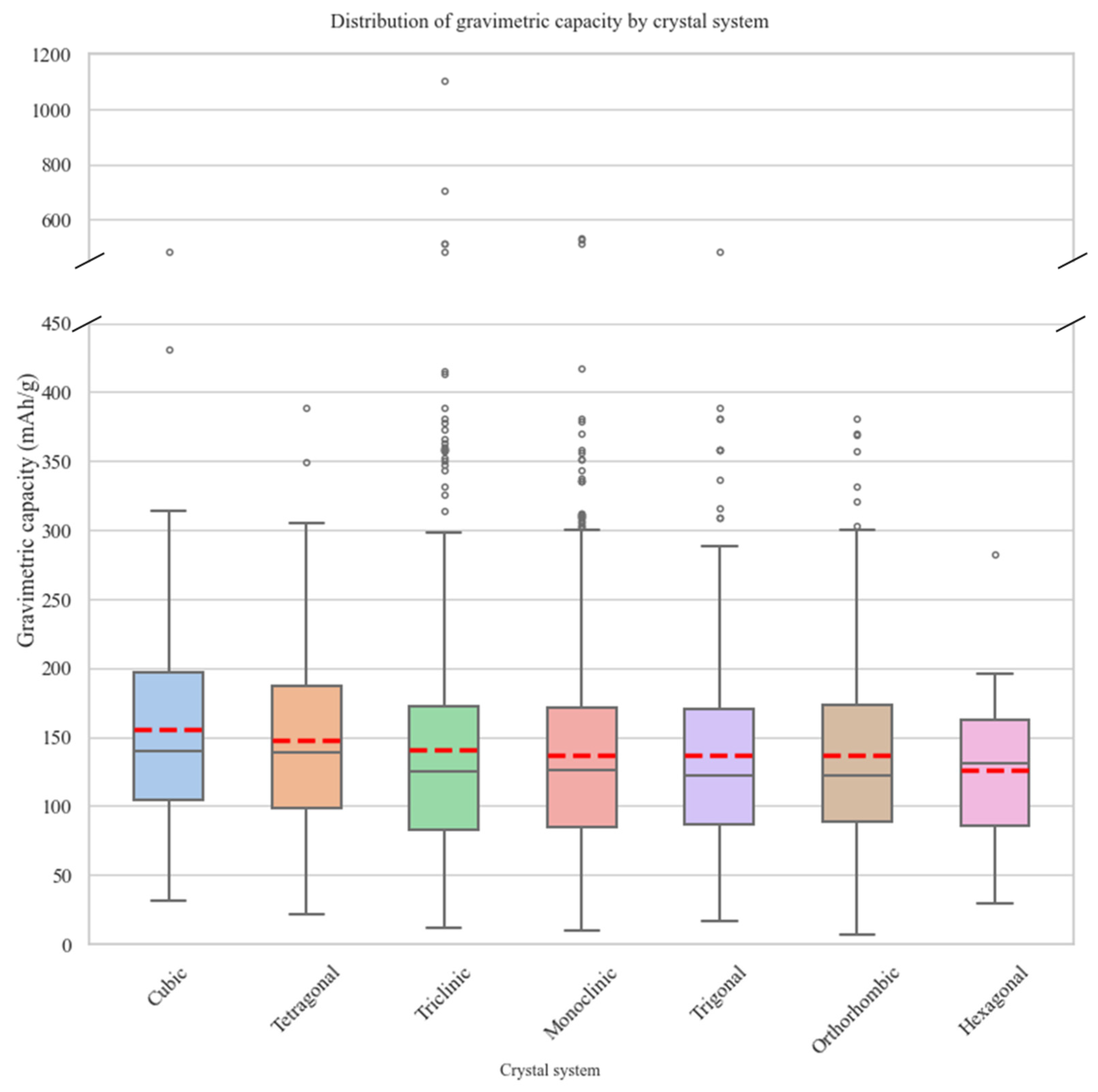
The crystal system classifies material structures based on symmetry and directly influences ionic diffusion pathways and lithium storage capacity. Cubic systems, known for high symmetry and three-dimensional diffusion channels, theoretically exhibit higher gravimetric capacity [29]. One-hot encoding was applied to represent each crystal system, enabling the model to discern capacity trends associated with crystal structure differences. To validate this approach, average gravimetric capacity was analyzed across crystal systems using 2424 cathode materials from the MP database. Consistent with theory, cubic systems exhibited the highest average capacity. Figure 2 presents box plots of capacity distributions for each crystal system, with red dashed lines indicating mean values arranged in descending order. This analysis demonstrates that crystal system information provides substantive explanatory power for capacity prediction, validating our structure-based feature design.

2.3. General Formula Embedding

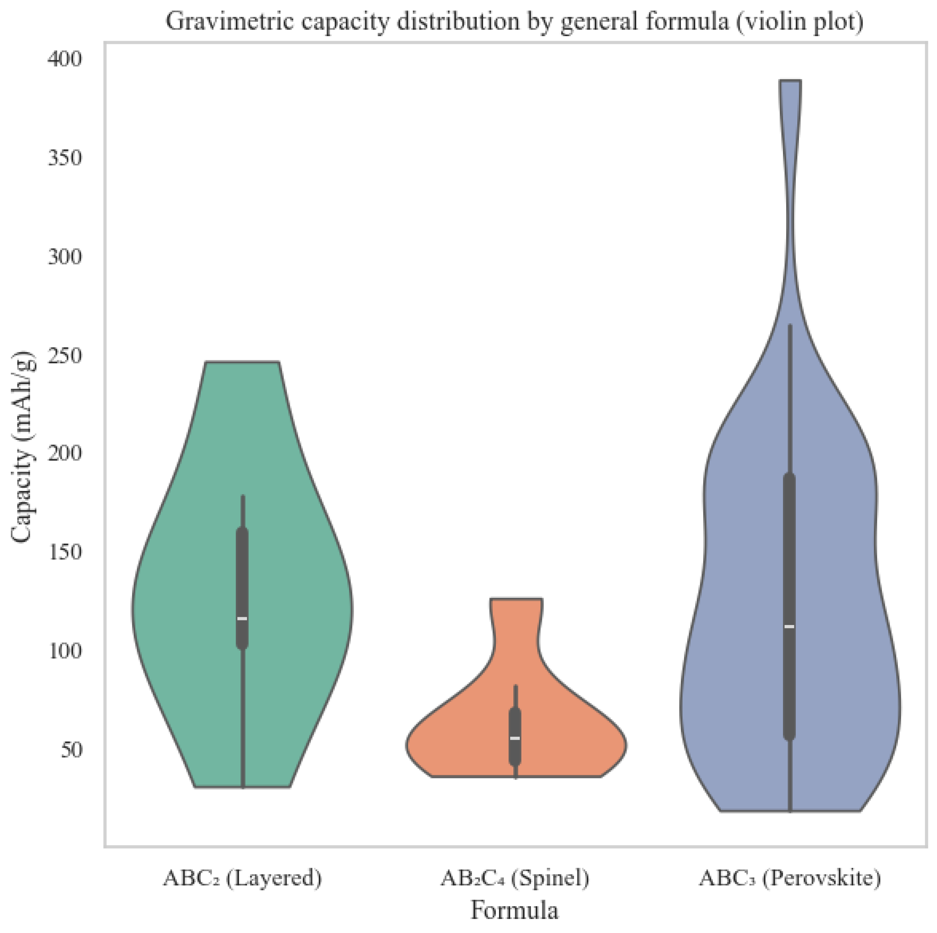
The general formula encodes the number of atoms at each crystallographic site, with available sites for ion insertion serving as a critical structural constraint on gravimetric capacity. For example, in spinel structures (AB₂C₄), lithium can only occupy A-sites, while B-sites remain fixed [30], restricting the maximum capacity. In this study, such structural constraints were explicitly encoded by quantifying site-specific atom counts. For instance, spinel AB₂C₄ is represented as (A = 1, B = 2, C = 4) as an input feature. This encoding preserves physical site information while enabling the model to learn ion accommodation capacity differences across structural types. Figure 3 presents the gravimetric capacity distribution for three representative general formula types (AB₂C₄, ABC₂, and ABC₃) based on the MP dataset, visualized as violin plots with kernel density estimation (KDE) [31]. Embedded box plots indicate median and interquartile range. These formulas correspond to spinel (AB₂C₄) [32], layered (ABC₂) [33], and perovskite (ABC₃) [34] structures, each exhibiting distinctly different capacity distributions: spinel structures show concentrated distribution in low-capacity regions, layered structures demonstrate intermediate capacity with a broad range, and perovskite structures display wide distribution extending to high-capacity regimes. These results demonstrate that general formulas effectively encode structural information beyond simple composition, reflecting differences in gravimetric capacity across structural types. Thus, general formulas serve as meaningful categorical features incorporating structural information, enabling AI models to learn structure–property relationships and contributing to effective training of complex crystal structure data.

2.4. Ion Type Embedding

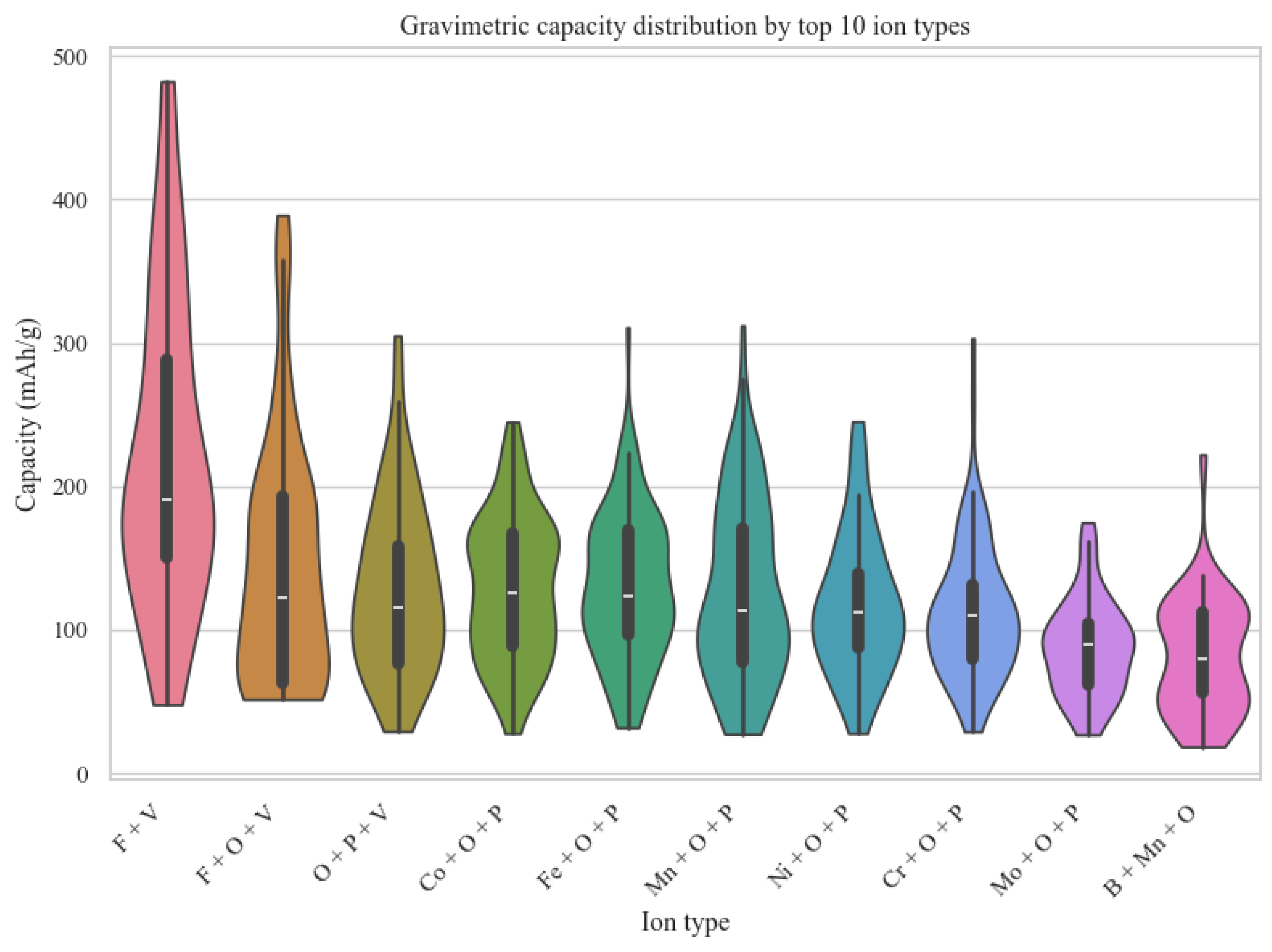
Ion type features reflect the combinations of transition-metal and nonmetal elements in cathode materials. Since capacity variations depend on the primary transition-metal constituents—such as Ni, Co, and Mn [35]—this study employed one-hot encoding to represent elemental presence (1 if present, 0 if absent). This approach enables the model to learn how element types and combinations influence capacity distribution. Figure 4 visualizes the gravimetric capacity distribution for the top 10 representative ion-type combinations using violin plots [31]. Each violin shape represents capacity distribution and density for materials with specific ion combinations, enabling intuitive comparison of differences in capacity and dispersion according to composition. Some ion-type combinations exhibit narrow, consistent capacity distributions, whereas others display wide ranges, suggesting that performance may vary significantly with compositional changes. These results demonstrate that composition-based features have a substantial impact on capacity prediction, highlighting the necessity for feature designs that effectively capture ion combination information.

2.5. Non-Negative Matrix Factorization (NMF)

The four categorical structural features—Formula, Crystal System, General Formula, and Ion Type—are individually transformed into numerical vectors through distinct embedding methods, resulting in a final 198-dimensional structure-based feature vector. However, such high–dimensional embeddings can entail the following challenges in terms of model training. First, string-based embedding approaches suffer from the sparsity issue, with most dimensions being zero, resulting in inefficient utilization of computational resources and low information density [36,37]. Second, due to the curse of dimensionality, increasing dimensionality dilutes feature density within the same data volume, posing an impediment to reliably learning generalized patterns. Therefore, feature extraction techniques or efficient reconfiguration of structural information are required to mitigate this issue [38].

To address this issue, this study implemented an NMF-based feature extraction technique [39]. Classical linear methods present fundamental limitations: (1) PCA’s orthogonal rotation generates negative components, obscuring the physical interpretability of latent factors in materials science contexts where features inherently represent non-negative material properties [40,41]; (2) ICA assumes statistical independence that is often incompatible with the correlations inherent in material properties [42]. Contemporary nonlinear approaches (UMAP, t-SNE) optimize for data visualization and manifold learning rather than explicit feature extraction, rendering extracted representations opaque for downstream supervised learning tasks and making them computationally prohibitive for high-dimensional structured data [43,44]. In contrast, NMF uniquely addresses these limitations through three key properties: (i) non-negativity constraints preserving the physical meaningfulness of latent factors, (ii) interpretable multiplicative decomposition directly revealing structural motifs, and (iii) explicit factorization enabling direct attribution of latent factors to material composition or structural features. Consequently, NMF provides superior suitability for materials informatics applications requiring both dimensionality reduction and physical interpretability of extracted features [45]. In the present work, the application of NMF reduced the total 198-dimensional structural feature vector to 98 dimensions based on manual tuning, as shown in

Table 2. Comparison of the data dimensions for each feature before and after employing NMF.

Feature Name	Dimension of Data
	Before NMF	After NMF
Formula	120	60
Ion Type	59	29
Crystal System	14	6
General Formula	5	3

.

This process preserved the primary patterns of the original data while effectively reducing feature redundancy. These dimensionally reduced structural features were subsequently utilized as an independent input branch in the model, enabling more efficient learning of the core patterns inherent in the structural information.

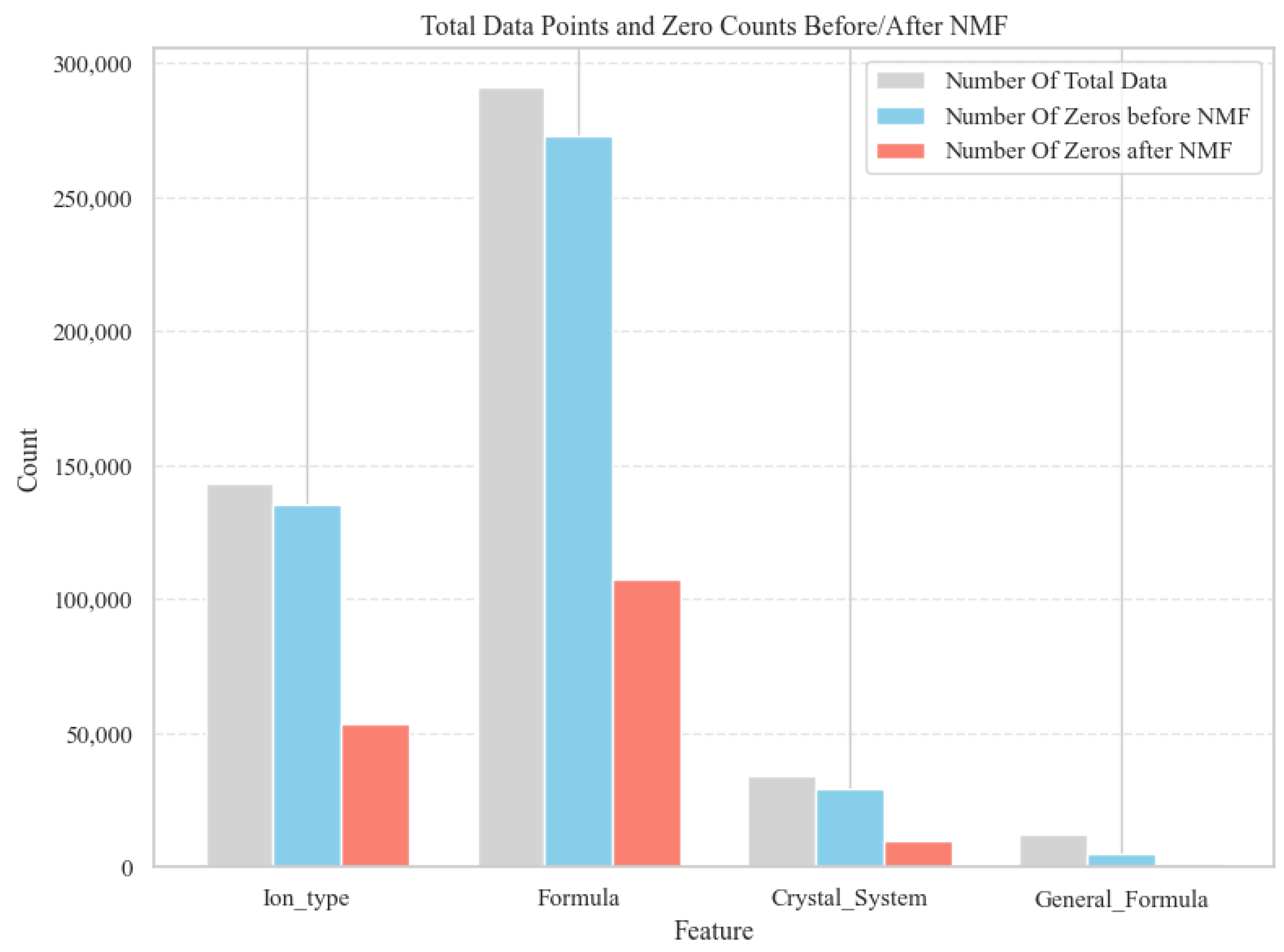
Figure 5 depicts a comparative analysis of total data counts and the distribution of zero values for four categorical input datasets before and after NMF-based dimensionality reduction following embedding. “Numbers of Total Data” denotes the total size of each input dataset, “Numbers of Zeros before NMF” indicates the number of zeros prior to dimensionality reduction, while “Numbers of Zeros after NMF” represents the number of zeros following dimensionality reduction.

Table 3. The related data of Figure 5.

Feature Name	Number of Total Data	Dimension of Data
		Before NMF	After NMF
Formula	290,880	272,799	102,760
Ion Type	143,016	135,607	52,415
Crystal System	33,936	29,088	10,512
General Formula	12,120	4711	1503

shows the detailed numerical values corresponding to the results in Figure 5. After reducing the dimensionality of each feature by half through NMF, the overall count of zero-valued elements decreased markedly, demonstrating that NMF-based feature extraction transforms high-dimensional, sparse inputs into a more compact, information-dense representation. Notably, the reduced proportion of zeros across all features indicates that NMF effectively captures nonlinear structural information, enabling the extraction of more cohesive and discriminative features. In this study, to effectively account for the sparsity of structural data and promote stable convergence, the “non-negative double singular value decomposition” (nndsvd) method was employed as the initialization strategy for NMF. By capturing dominant feature patterns in highly sparse input matrices from the early stages of decomposition, this initialization strategy facilitates the more efficient extraction of latent structural factors [46].

3. Proposed Methodology: Classified Branch–CapNet

3.1. Stochastic Analysis for Optimized Training Architecture Design

Traditional deep learning architectures predominantly adopt a simplistic concatenation strategy, wherein all input features are naively integrated into a monolithic vector representation for model training. However, the structural embedding data employed in this investigation exhibit inherently sparse and high-dimensional characteristics, while the numerical chemical property features manifest as dense and low-dimensional vectors, with fundamentally divergent statistical distributions and scaling properties. The integration of such heterogeneous data modalities through conventional single pathway learning approaches exacerbates the semantic gap, potentially resulting in suboptimal model performance and compromised predictive accuracy [47].

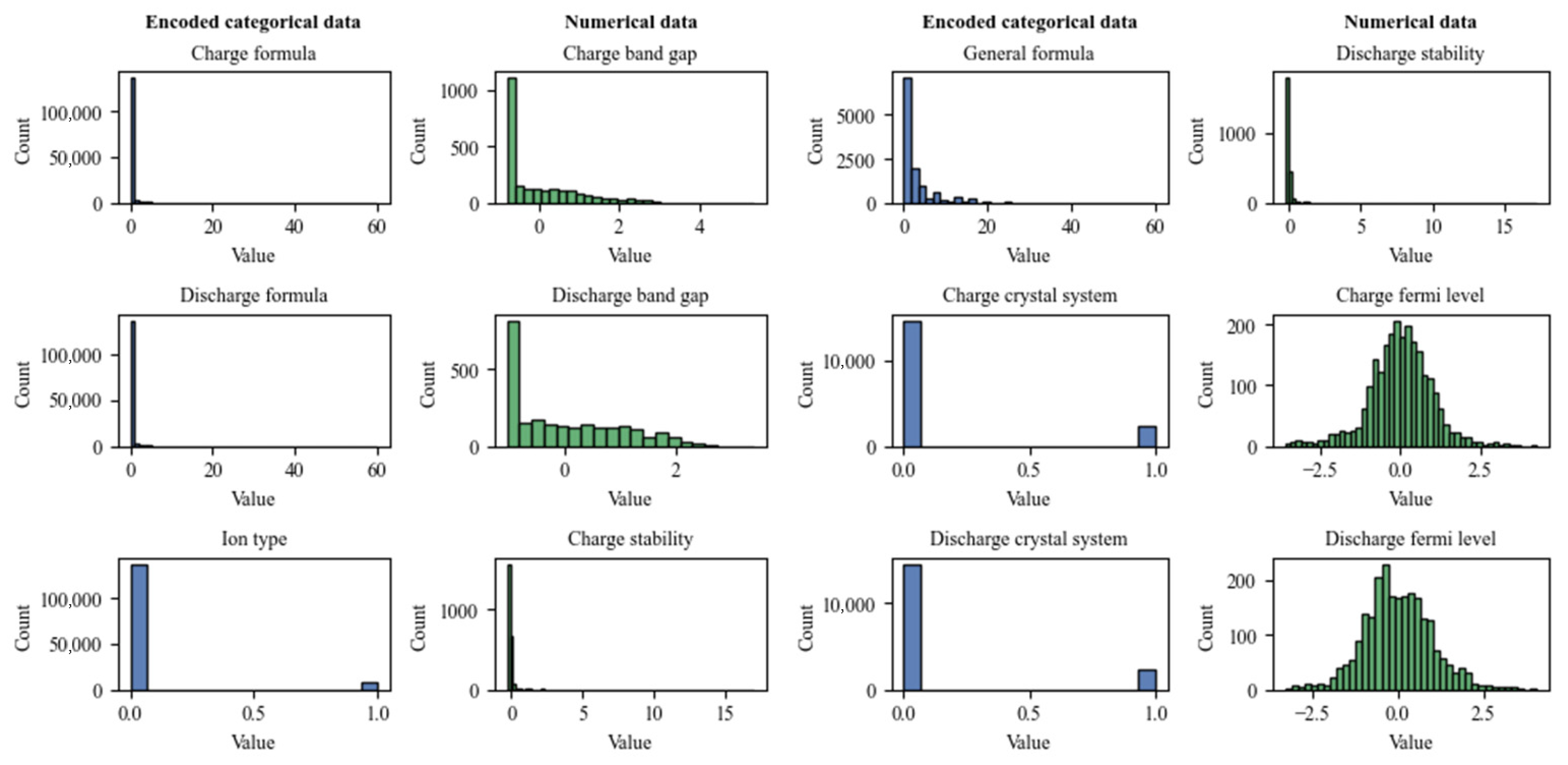
Figure 6 presents visually compares the value distributions for categorical and numerical features used in model training. The blue histograms on the left depict the encoded categorical data: both the crystal system and ion type features, after one-hot encoding, exhibit values concentrated at 0 and 1. The Formula data, which directly reflect the number of atoms in each molecule, show a wide distribution ranging (0 to 60), although a substantial proportion of values are concentrated near 0. In contrast, the green histograms on the right represent the numerical data, which-except for stability-display continuous distributions and exhibit a relatively narrower overall range, compared to the formula data.

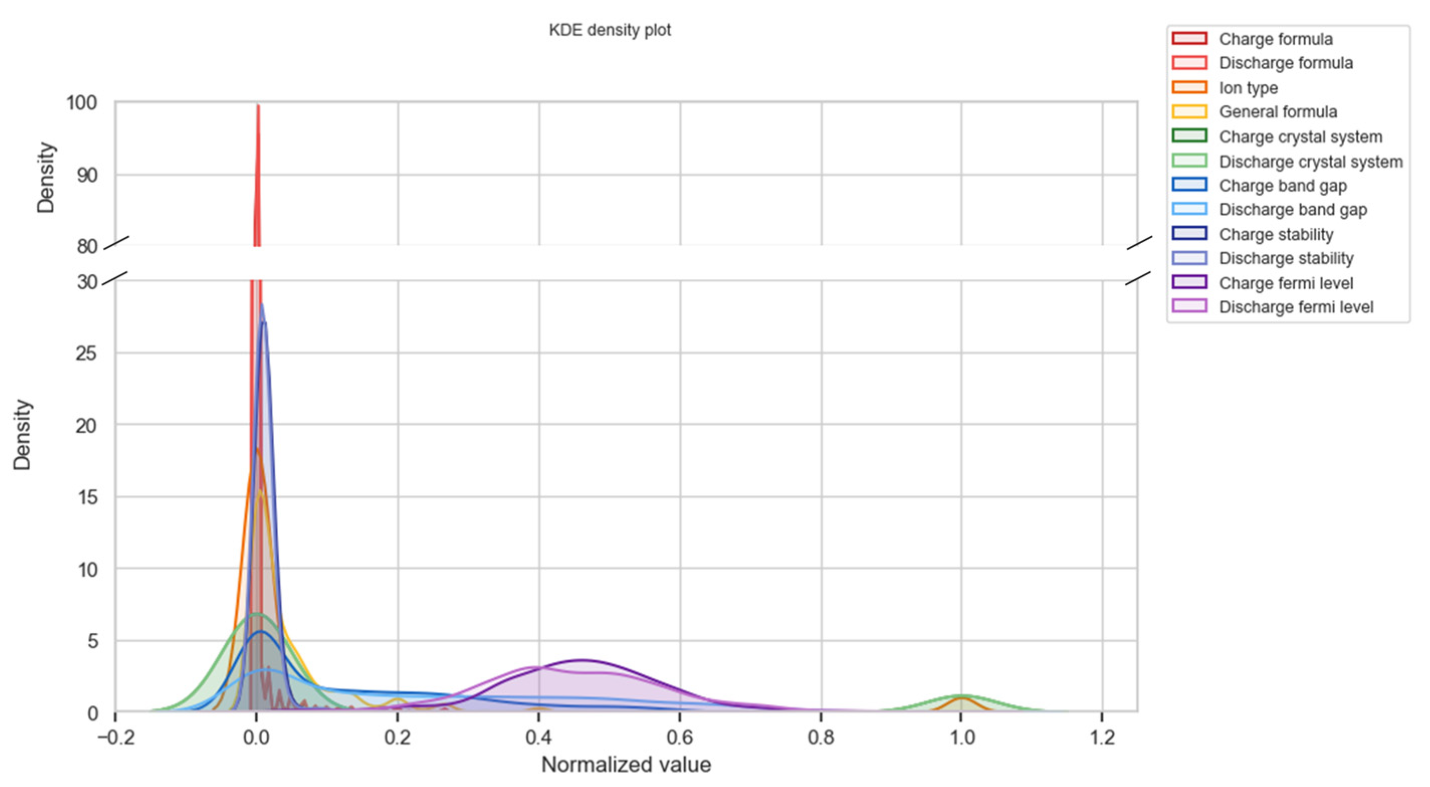
Figure 7 presents the kernel density estimation (KDE) visualization of categorical and numerical data distributions. All feature values on the X-axis are scaled to the 0–1 range using min–max normalization, while the Y-axis employs a broken axis technique to simultaneously display extremely high-density values. For the categorical data, both the crystal system and ion type show distributions concentrated in the 0 and 1 intervals as a result of one-hot encoding, whereas formula-related data are predominantly concentrated near zero. In contrast, the numerical data demonstrate continuous value distributions, with ranges and distributional characteristics that are markedly different from those of the categorical data. Although the KDE visualization is based on normalized values, direct absolute numerical comparisons are not feasible; however, the statistical distribution differences between the two data types are evident. Applying conventional deep learning models that process categorical and numerical data through a single path without considering these differences may result in insufficient learning of the structure–property relationships inherent in each data type, potentially leading to performance degradation. This comprehensive analysis demonstrates the necessity for strategic learning approaches that appropriately classify input data and direct each type through optimized forward propagation pathways.

3.2. Classified Branch–CapNet Architecture

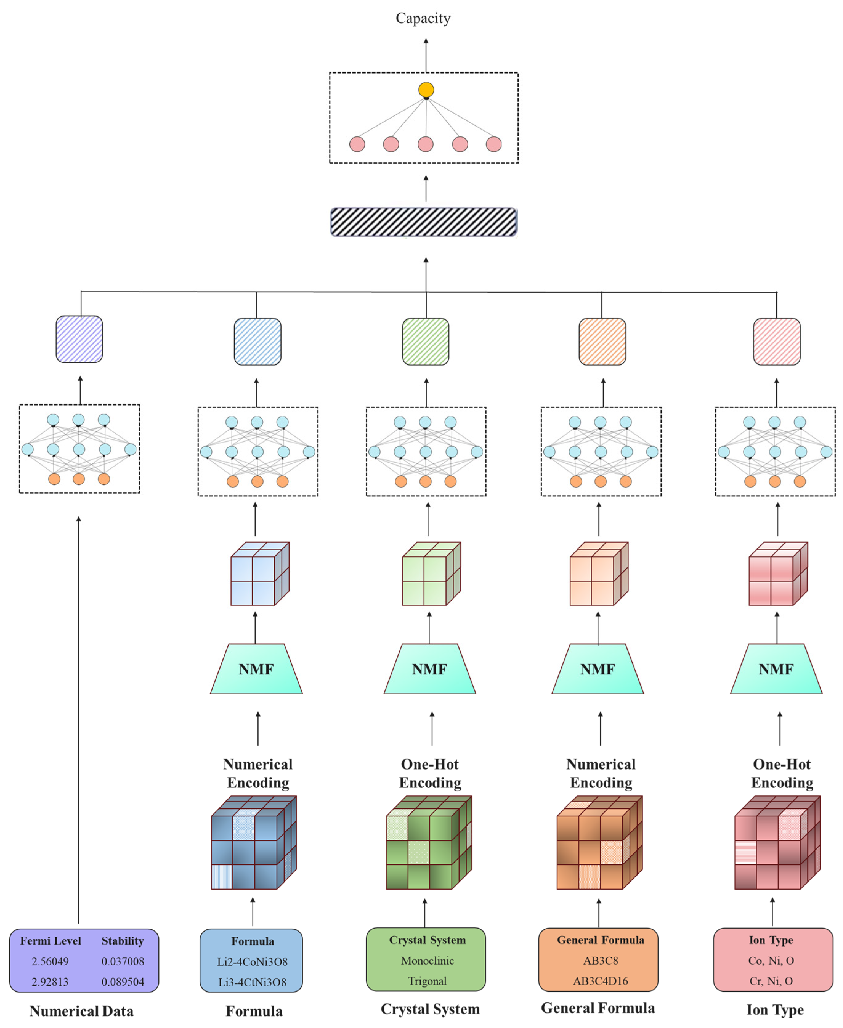
This study proposes effective architecture that comprises five independent input branches to account for the statistical differences between structure-based categorical data and the numerical chemical data identified in Section 2. By explicitly minimizing inter-feature interference, the model can more precisely learn the relationships between each input modality and the target capacity. Figure 8 illustrates the overall architecture of the proposed network. The model processes the embedded categorical structural data and numerical data through separate classified branches with distinct networks, which are ultimately integrated using a late fusion strategy. This design minimizes inter-feature interference and enhances the accuracy of capacity prediction.

Table 4. The architectural design of the proposed model network corresponds to the input.

Feature Name	Input Layer	Hidden Layer 1	Hidden Layer 2
Formula	60	600	300
Ion Type	6	60	30
Crystal System	3	30	15
General Formula	29	290	145
Numerical Data	6	60	30

details the input dimensions for each data modality, the composition of the hidden layers within each branch, and the architecture of the final integration layer following concatenation.

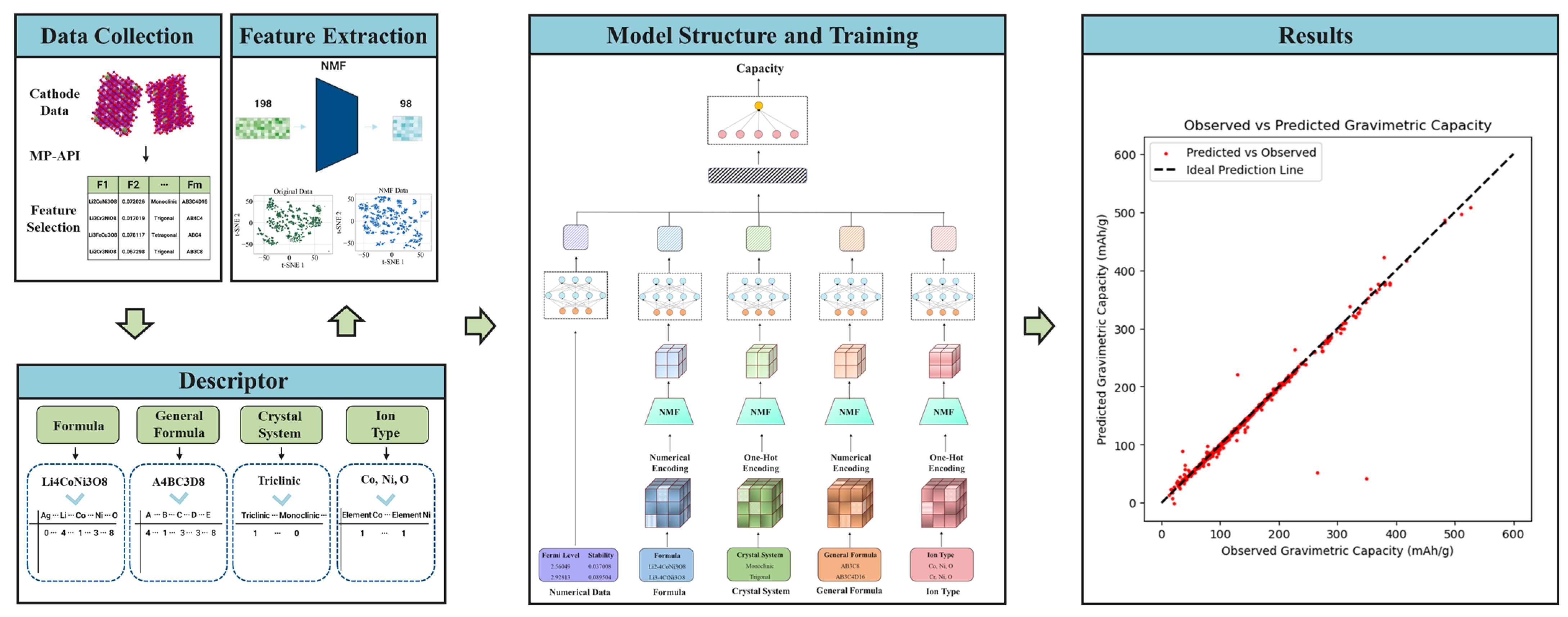
Figure 9 illustrates the complete data processing workflow from raw cathode material features extracted from the Materials Project database through to final capacity predictions. Input vectors are systematically extracted and constructed, followed by optimized embedding and dimensionality reduction processes. The preprocessed features are subsequently processed through the Classified Branch–CapNet architecture, wherein categorical and numerical data streams are independently processed through dedicated branches. During training, the model undergoes forward and backward propagation to optimize network parameters, ultimately generating accurate gravimetric capacity predictions as the final output.

After passing NMF, each input branch independently traverses two hidden layers. In each branch, the first hidden layer comprises ten times the number of input features, facilitating the learning of rich, high-dimensional representations. The second hidden layer is then reduced to half the size of the first, enabling a gradual learning process for feature representation. This hierarchical dimensionality reduction design is optimized to effectively suppress noise inherent in high-dimensional sparse embeddings while preserving salient patterns. The five branch-specific representation vectors are subsequently merged via a late fusion concatenation process, and then fed into the final layer. In this stage, the integrated vector passes through a fully connected network, and the output nodes predict the target material capacity. The proposed late fusion approach offers superior flexibility in handling heterogeneous data sources by assigning modality-specific weights that are proportional to their information content [48]. In the context of gravimetric capacity prediction, the chemical formula feature contributes the greatest information density, and is thus leveraged most effectively, while additional modalities can be seamlessly incorporated to enhance model extensibility [49]. By first allowing each feature group to learn its independent feature–target relationship, and subsequently integrating these embeddings within a unified feature space, this architecture alleviates the semantic gap commonly observed in conventional fully connected structures, while also more accurately capturing the complementary information across diverse data types. The output value of the $i$-th neuron in the deep neural network (DNN) is formulated as follows [50]:

$$h_i = \mathrm{ELU}(\sum _{j=1}^n{w}_{ij}{x}_j+b_i)$$

(1)

Table 5. Symbol definitions for equations.

Symbol	Meaning	Dimension/Domain
$h^k$	$\mathrm{Hidden} \mathrm{layer} \mathrm{output} \mathrm{from} \mathrm{branch} k$	${\mathbb{R}}^{d_1}$
$w_{ij}^k$	$\mathrm{Weight} \mathrm{parameter} \mathrm{connecting} j$$\text{-}\mathrm{th} \mathrm{input} \mathrm{to} i$$\text{-}\mathrm{th} \mathrm{layer} \mathrm{of} \mathrm{branch} k$	Scalar
$x_j^k$	$j$$\text{-}\mathrm{th} \mathrm{NMF}\text{-}\mathrm{preprocessed} \mathrm{input} \mathrm{feature} \mathrm{for} \mathrm{branch} k$	Scalar
$b_i^k$	$\mathrm{Bias} \mathrm{term} \mathrm{for} i$$\text{-}\mathrm{th} \mathrm{layer} \mathrm{of} \mathrm{branch} k$	Scalar
$n_k$	$\mathrm{Number} \mathrm{of} \mathrm{NMF} \mathrm{components} \mathrm{for} \mathrm{branch} k$	Integer
$d_1=10\times n_k$	First hidden layer dimension	Integer
$d_2=d_1/2$	Second hidden layer dimension	Integer
ELU(·)	Exponential Linear Unit activation function	-
$k$	Branch index	{F, C, G, I, N}
$i$	Layer index	{1, 2}

presents comprehensive definitions of the symbols employed in the equations throughout the manuscript.

The five embedded data streams independently pass through two hidden layers, with their outputs prior to concatenation are as follows in Equations (2)–(6):

$$h^{\mathrm{F}} = \mathrm{ELU}(\sum w^{\mathrm{F}}{x}^{\mathrm{F}}+b)$$

(2)

$$h^{\mathrm{C}}=\mathrm{ELU}(\sum w^{\mathrm{C}}{x}^{\mathrm{C}}+b)$$

(3)

$$h^{\mathrm{G}}=\mathrm{ELU}(\sum w^{\mathrm{G}}{x}^{\mathrm{G}}+b)$$

(4)

$$h^{\mathrm{I}}=\mathrm{ELU}(\sum w^{\mathrm{I}}{x}^{\mathrm{I}}+b)$$

(5)

$$h^{\mathrm{N}}=\mathrm{ELU}(\sum w^{\mathrm{N}}{x}^{\mathrm{N}}+b)$$

(6)

where F, C, G, I and N denote Formula, Crystal system, General formula, Ion type and Numerical data, respectively. Following concatenation, the hidden vectors from each branch are merged into a single final vector, as expressed in Equations (7) and (8):

$$h^{\mathrm{F}\mathrm{u}\mathrm{s}\mathrm{i}\mathrm{o}\mathrm{n}} = [h^{\mathrm{F}}\oplus h^{\mathrm{C}}\oplus h^{\mathrm{G}}\oplus h^{\mathrm{I}}\oplus h^{\mathrm{N}}]$$

(7)

$$h^{\mathrm{F}\mathrm{i}\mathrm{n}\mathrm{a}\mathrm{l}}= \mathrm{Linear}\left(\sum w^{\mathrm{F}\mathrm{u}\mathrm{s}\mathrm{i}\mathrm{o}\mathrm{n}}{h}^{\mathrm{F}\mathrm{u}\mathrm{s}\mathrm{i}\mathrm{o}\mathrm{n}}+b\right)$$

(8)

4. Results and Discussion

4.1. Training Configuration

The complete dataset (2424 samples) acquired from the Materials Project (MP) database was partitioned into training (1697 samples) and testing sets (727 samples) in a 7:3 ratio. Prior to training, structural embedding, preprocessing procedures, and NMF-based feature extraction were executed sequentially. Model training and evaluation were conducted on a computing system comprising a 12th Gen Intel^® Core™ i5–12400F CPU, 16 GB RAM, and an NVIDIA GeForce GTX 1660 SUPER GPU (boost clock 1815 MHz, 1408 CUDA cores, 6 GB GDDR6 memory, 336.05 GB/s memory bandwidth). The software environment consisted of Python 3.10.0, TensorFlow 2.10.0, and CUDA 11.2.

Table 6. Hyperparameter configuration for all training processes in this work.

Hyperparameter	Configuration(Tuning Range)	Description
Optimizer	Adam	Adaptive moment estimation optimizer
Learning Rate	$1\times {10}^{-4}$$({10}^{-1}$$~{10}^{-5}$)	Initial learning rate
Batch Size	100 (10~1000)	Mini-batch size used for training
Loss Function	Mean Squared Error	Regression loss function
Dropout	0.2 (0.1~0.5)	Applied after each hidden layer
Activation Function	ELU	Exponential Linear Unit for all hidden layers
Weight Initialization	TensorFlow default	No customized initialization
Epoch	2300 (1000~3000)	One complete pass of the entire training dataset

presents the complete hyperparameter configuration employed in all training processes, including the exploration ranges used during optimization. Within these specified ranges, a systematic grid search strategy was conducted to identify the optimal hyperparameter values. The detailed specifications of the final hyperparameter settings are as follows: (1) The learning rate was optimized over the range [$1\times {10}^{-1}$~$1\times {10}^{-5}$], with $1\times {10}^{-4}$ selected as the optimal value; (2) batch size was systematically evaluated across [10, 100, 1000], with 100 determined as the optimal configuration; (3) dropout rate was tuned within the range [0.1 ~ 0.5] to avoid overfitting, with 0.2 selected for the final model; (4) training epochs were optimized over [1000 ~ 3000], with 2300 epochs determined as the optimal setting. Additionally, the Exponential Linear Unit (ELU) activation function was employed to ensure stable convergence during training, and weight initialization was performed using TensorFlow’s Glorot Uniform initialization strategy to facilitate effective model learning.

4.2. Evaluation Metrics

Model performance was comprehensively evaluated using three complementary metrics: Mean Absolute Error (MAE), Root Mean Square Error (RMSE), and Coefficient of Determination (R²). MAE measures the average of absolute differences between predicted and actual values, retaining the original units (mAh/g) and enabling intuitive interpretation of prediction errors [51]. Complementarily, RMSE quantifies the overall deviation between predicted and actual values while penalizing larger errors more heavily than MAE, making it particularly useful for assessing model robustness and stability [52]. Finally, R² evaluates the proportion of variance in actual data explained by model predictions, providing a relative measure of how well predicted values approximate true values. An R² closer to 1 indicates superior model generalization and higher predictive accuracy [53]. The three metrics are defined as follows:

$$\mathrm{MAE}= {\displaystyle \frac{1}{n}}\sum _{i=1}^n\left|y_i-{\widehat{y}}_i\right|$$

(9)

$$\mathrm{RMSE} = \sqrt{{\displaystyle \frac{1}{n}}\sum _{i=1}^n{\left(y_i-{\widehat{y}}_i\right)}^2}$$

(10)

$${ \mathrm{R}}^2= 1-{\displaystyle \frac{{\sum _{i=1}^n({\widehat{y}}_i-\overline{y})}^2}{{\sum _{i=1}^n(y_i-\overline{y})}^2}}$$

(11)

where, for MAE and RMSE: $y_i$ denotes the true value, ${\widehat{y}}_i$ represents the predicted value, and $n$ indicates the number of samples. For R²: $\overline{y}$ indicates the mean of observed (true) values. Lower MAE and RMSE values indicate better performance, while R² values closer to 1 reflect higher predictive accuracy and model generalization capability.

4.3. Building of the Classified Branch–CapNet Architecture

The proposed model was implemented as a multi-branch deep learning architecture that processes different types of input features through independent fully connected layer pathways, and ultimately integrates them for prediction. The input data are categorized into five modalities: Ion Type, Formula, Crystal System, General Formula, and Numerical Data, with each modality being independently learned through separate pathways. Table 4 (Section 3.2) shows that the Ion Type pathway receives 29-dimensional input, and sequentially passes through 290 units and 145 units, while the Formula pathway receives 60-dimensional input, and passes through 600 units and 300 units. The Crystal System pathway receives 6-dimensional input and passes through 60 units and 30 units, while the General Formula pathway processes 3-dimensional input through 30 units and 15 units. The Numerical Data pathway receives 6-dimensional input, and passes through 60 units and 30 units. To ensure training stability and generalization performance, all hidden layers in the pathways employ ELU activation functions and a dropout rate of 0.2. The embedding vectors extracted from each branch are concatenated into a single vector. The fused vector is then fed into the output layer, which comprises a hidden layer of five nodes, followed by an output layer of one unit to generate the result. Since the proposed model independently learns modality-specific features before integration, it can effectively capture interactions between structural features and chemical properties. This enables more precise representation learning, compared to conventional models that simply process all inputs as a single vector.

Determination of Input Feature Multiples to Optimize Hidden Layer Structure

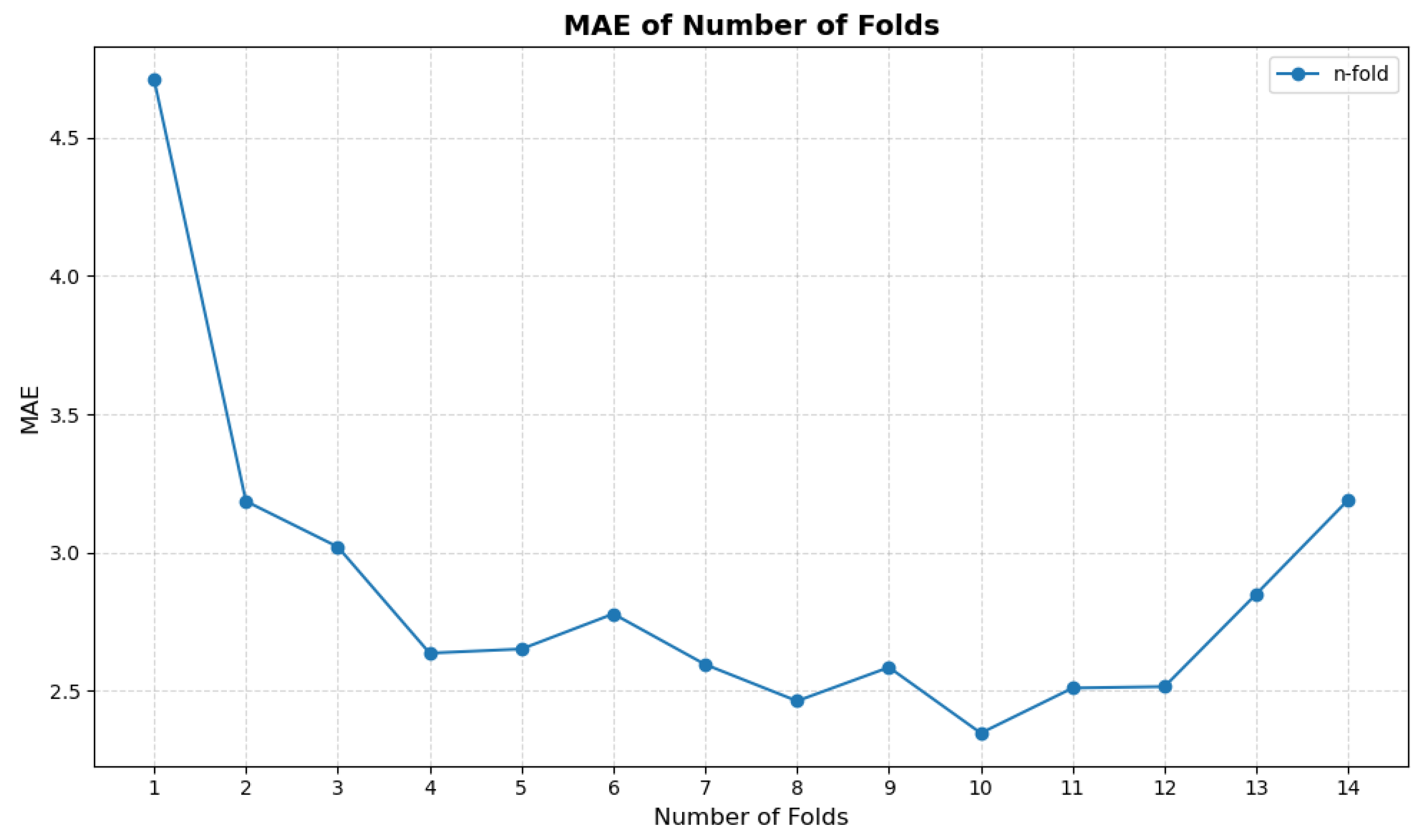
To evaluate the impact of hidden-layer architectures on model performance and identify the optimal configuration, we varied the number of nodes in the first hidden layer from 1× to 14× the input dimensionality for each branch, and compared the resulting mean absolute error (MAE). The second hidden layer was fixed at half the size of the first to preserve key patterns, while effectively reducing the noise inherent in high-dimensional sparse embeddings. Figure 10 illustrates the performance differences, measured by MAE, when the number of nodes in the first hidden layer is set to n–fold multiples of the input dimension.

Table 7. The related data of Figure 10 (displayed in 2-fold increments).

Number of Folds	2-fold	4-fold	6-fold	8-fold	10-fold	12-fold	14-fold
MAE	3.186	2.637	2.779	2.464	2.348	2.516	3.191

summarizes the MAE results for experiments using even–fold numbers. Overall, increasing the hidden-layer size relative to the input dimension led to reduced MAE and improved performance. The lowest MAE of 2.348 was achieved with the 10–fold structure, indicating optimal predictive performance. Although larger hidden layers enhanced model’s representational capacity and training performance, MAE increased again beyond the 10-fold configuration, suggesting overfitting or training instability due to excessive model complexity. Hence, the 10-fold design proposed in this study offers the optimal balance between performance improvement and generalization.

4.4. Comparative Baseline Methods

To quantitatively assess the performance of the proposed model, we conducted comparative experiments against several baseline models that are commonly used in the related works. For fair comparison, each baseline was configured with three hidden layers and adjusted to approximately 270 K parameters to match the proposed model’s computational cost, enabling a direct performance comparison under similar resource constraints.

4.4.1. Deep Neural Network (DNN)

As the first comparison benchmark, we constructed a baseline model using a DNN architecture that offers the advantages of simple implementation and fast training time [16]. The baseline DNN model concatenates all 98 input features into a single vector and sequentially processes it through three fully connected layers. The input layer consists of 98 units without activation functions or dropout. The first hidden layer contains 589 units, the second hidden layer has 294 units, and the third hidden layer includes 147 units, with all hidden layers employing ELU activation functions and 0.2 dropout. The final output layer comprises a single unit with a linear activation function.

4.4.2. Recurrent Neural Network (RNN)

In this study, we introduce RNN as a comparative baseline to capture elemental interactions (both global and local interactions) within compounds based on the embedding representations of elemental and stoichiometric information [54]. Each cathode material sample represents an independent data point requiring the prediction of a single output (capacity value). Unlike conventional time series data that can be extended across multiple time steps, the structural characteristic of materials data precludes temporal expansion. Consequently, all input features are transformed into sequences with a length of one for RNN processing. This configuration does not aim to learn actual temporal dependencies, but rather serves as a comparative baseline to experimentally validate how the structural differences between our proposed model and RNN impact prediction performance under equivalent conditions. That is, the RNN baseline enables systematic evaluation of model architectures for materials property prediction tasks where sequential processing may capture complex elemental interactions, despite the absence of an inherent temporal relationship. The configuration of the RNN model for comparison consists of an input layer with 98 units, with no activation function or dropout applied. The first hidden layer is composed of a SimpleRNN with 352 units, followed by the second hidden layer with 176 units, and the third hidden layer with 88 units, in sequential connection. All three hidden layers utilize hyperbolic tangent (tanh) as the activation function, and apply an identical dropout rate of 0.2. The final output layer consists of a single unit and employs a linear activation function.

4.4.3. Long Short-Term Memory (LSTM)

LSTM is an algorithm that introduces gating mechanisms to ameliorate the gradient vanishing and exploding problems inherent in RNN, demonstrating sensitivity to short-range information correlations, while better capturing long-range interactions between elements [55]. The gating mechanisms within LSTM cells enable the selective retention and forgetting of information, which is particularly advantageous for modeling complex chemical relationships where certain elemental combinations may exhibit stronger correlations than others. For the same reason as the RNN, this model transforms all input features (98 dimensions total) into sequences with a length of one, and feeds them into three consecutive LSTM layers. The architecture for comparative experiments features an initial layer of 98 units, without activation or dropout mechanisms. Subsequently, three LSTM hidden layers are implemented with decreasing unit counts of 165, 82, and 41 units, respectively. Each hidden layer incorporates hyperbolic tangent (tanh) activation, with uniform dropout regularization set at 0.2. The output layer contains a single unit utilizing linear activation for regression output.

4.4.4. Encoder-Only Transformer

The encoder-only Transformer was employed as one of the comparative architectures. Unlike the standard Transformer, which consists of both an encoder and a decoder, this model adopts only the encoder component since the task involves predicting a gravimetric capacity rather than generating a sequential output [56]. A decoder, which typically requires the addition of a begin-of-sequence (BOS) token to initiate sequence generation, is unnecessary here because the input does not represent sequential or temporal data. Instead, the input comprises a fixed 98-dimensional feature vector that encodes chemical composition, crystal system, and related electronic descriptors. As these features do not possess sequential dependencies or token order, the use of a BOS token would be physically and chemically meaningless, and an autoregressive decoding process would only introduce redundant computational overhead. Therefore, only the encoder blocks were utilized to capture latent inter-feature dependencies and structural correlations within the material descriptors. The overall architecture consists of three main components: an input projection layer, an encoder stack, and a regression head. The input projection layer transforms the 98-dimensional feature vector into the Transformer’s embedding dimension through a sequence of Dense–LayerNormalization–ELU–Dropout operations. This stage normalizes features with differing numerical scales, enhances nonlinear expressiveness through the ELU activation, and improves generalization via dropout regularization. The resulting embedding, reshaped into a sequence of length one, is processed through multiple encoder blocks. Each encoder block is composed of a Multi-Head Self-Attention mechanism, a Feed-Forward Network (FFN), Layer Normalization, and Residual Connections. The self-attention module captures interdependencies among features—such as correlations between ion type, chemical formula, and crystal system—by learning contextualized representations across all dimensions simultaneously. The FFN expands and refines these representations through nonlinear transformations, while Layer Normalization and residual pathways stabilize gradient flow and promote efficient convergence. In this study, two encoder layers were employed to progressively deepen the representation of inter-feature relationships. Following the encoder stack, the regression head, composed of LayerNormalization–Dense–Dropout–Dense, aggregates the encoded representation and outputs a single scalar prediction via a linear activation function. The dropout rate was set to 0.2 to mitigate overfitting, and optimization was performed using Adam. The model’s hyperparameters were configured as follows: the model dimension was set to 86, the number of attention heads to 4, the number of encoder layers to 2, the feed-forward network dimension to 64, and the dropout rate to 0.2. These settings constrain the total number of trainable parameters to approximately 270,000, ensuring parity in model complexity with other comparative architectures. This allows for a fair evaluation of predictive performance attributable solely to the architectural advantages of the Transformer, particularly its self-attention mechanism for modeling complex inter-feature dependencies. Consequently, the encoder-only Transformer effectively captures structural correlations among material descriptors while maintaining a compact and computationally efficient design optimized for regression tasks.

4.5. Performance Comparison

Table 8. Performance comparison of comparative deep-learning models for capacity estimation errors including computational cost.

Model	Average MAE (1)	Max MAE	Min MAE	Average RMSE (1)	Max RMSE	Min RMSE	R2	Total Parameters	Computational Time (2)
DNN	5.569	6.104	5.335	16.333	16.840	16.141	0.956	275,284	0:01:15
RNN	8.484	9.063	8.107	16.101	17.416	15.701	0.957	275,265	0:03:01
LSTM	9.351	9.970	9.232	17.377	18.147	17.072	0.950	275,962	0:03:58
Encoder-only Transformer	4.992	5.179	4.325	17.003	21.371	16.092	0.952	274,555	0:19:09
Proposed Model	2.441	2.552	2.261	15.236	15.411	15.125	0.961	275,491	0:01:49

⁽¹⁾ Average of 20 experiments. ⁽²⁾ Computational time refers to the sum of training and inference time (seconds).

presents a comparative analysis of the MAE, RMSE, R², total parameter count and computational time between the proposed model and benchmark models, including DNN, RNN, LSTM and the encoder-only architectures. Each model underwent 20 independent experimental trials, and the average MAE values were calculated based on these experimental results. All comparative models were configured to maintain similar total parameter counts to the proposed model, ensuring fair evaluation of predictive performance differences that were attributable to architectural variations. The experimental results demonstrate that the proposed classified branch-based model achieved a mean MAE of 2.441, representing substantial prediction error reductions of (56.2, 71.2, 73.9, and 51.1) %, compared to the DNN, RNN, LSTM, and encoder-only Transformer models, respectively. Furthermore, the proposed model achieved the lowest average RMSE of 15.236, corresponding to reductions of 6.7%, 5.4%, 12.3%, and 10.4% relative to the DNN, RNN, LSTM, and encoder-only Transformer models, respectively. In addition, it recorded the highest coefficient of determination of 0.961, outperforming all comparative models (0.956, 0.957, 0.950, and 0.952). These findings establish the superior predictive performance of the proposed methodology across all the evaluated benchmark architectures. The DNN model, built by merely concatenating all inputs, achieved a stable MAE of 5.569 and an average RMSE of 16.333, with a coefficient of determination of 0.956, but is inherently limited by its inability to capture the distinct statistical properties of individual input features. Moreover, RNN and LSTM models recorded MAE values of (8.484 and 9.351), average RMSE values of 16.101 and 17.377, and coefficients of determination of 0.957 and 0.950, respectively, demonstrating degraded performance, despite utilizing recurrent architectures. Although RNN and LSTM models exhibit strong capabilities in capturing global and long-range interactions between elements in the transformed elemental and stoichiometric data, the deteriorated generalization performance can be attributed to the semantic gap phenomenon caused by the heterogeneous statistical properties between numerical and categorical data of cathode materials, which impedes effective learning through simple concatenation approaches [54]. In contrast, the proposed model processes input features with distinct statistical properties in separate branches before integration, thereby minimizing inter-feature interference and enabling each feature’s characteristics to be learned effectively. As a result, it achieves substantial improvements in predictive performance without increasing structural complexity, supporting the efficacy of the classified-branch architecture for materials data with heterogeneous features [57]. In terms of computational cost, comparative analysis shows that our proposed Classified Branch–CapNet model achieves superior performance while maintaining comparable computational cost compared to baseline models. Notably, when compared to the encoder-only Transformer model, our approach requires only 10% of the computational cost while demonstrating 50% error reduction.

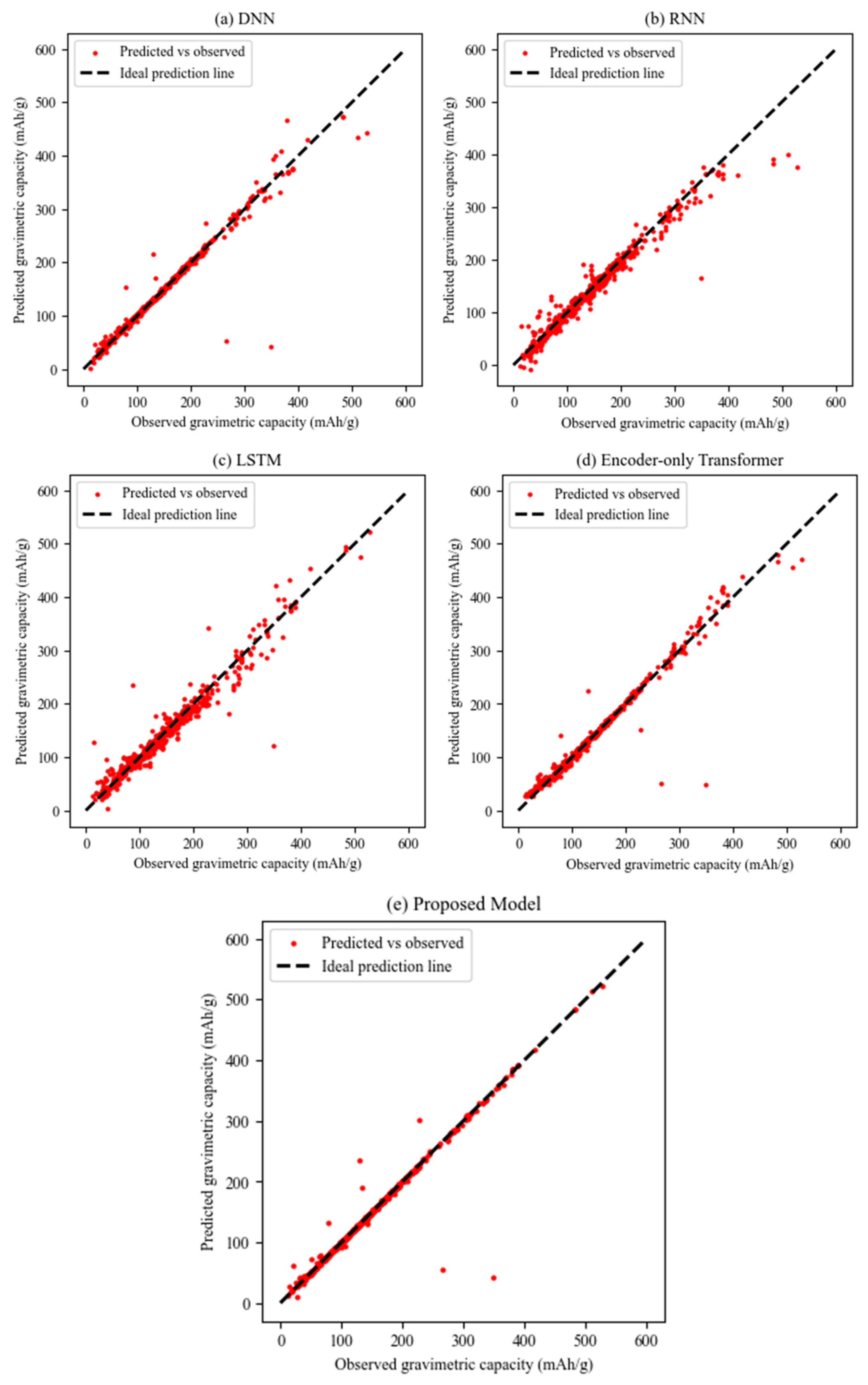
In Figure 11a, most samples cluster near the reference line, indicating generally accurate predictions. Figure 11b,c show that the RNN and LSTM models produce a wider spread of points farther from the reference line, reflecting higher variance in their predictions. Figure 11d presents that the encoder-only Transformer achieves better alignment along the ideal prediction line than the DNN-, RNN-, and LSTM-based models, confirming its superior representation capability and improved overall accuracy. However, for all four models (a–d), the predictive performance tends to decline in the high-capacity region (>300 mAh/g), suggesting limited generalization to extreme values. These results underscore the necessity of a learning strategy that accounts for the distinct statistical properties of numerical and categorical data. Specifically, the proposed model addresses these limitations by classifying and independently training features with differing statistical characteristics, and then applying a late-fusion strategy. Experimental results demonstrate that its predictions closely align with the reference line across the entire capacity range and maintain consistent accuracy even in high-capacity regions. This suggests that isolating heterogeneous features before fusing them effectively reduces inter-feature interference and contributes to improved predictive performance.

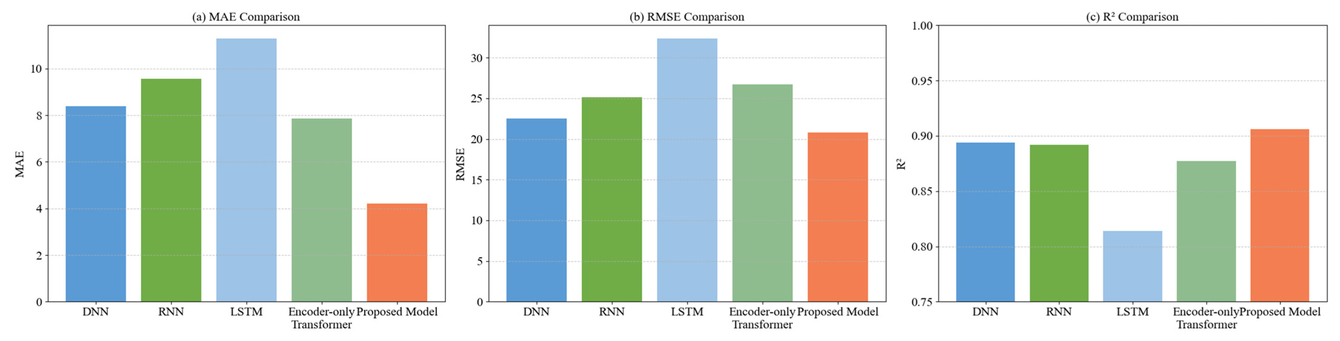
To enhance the generalization performance and reliability of the proposed model, cross-validation was conducted. Given that the Materials Project database exhibits imbalanced class distributions across cathode material categories, Stratified K-Fold cross-validation was employed to rigorously evaluate the model’s generalization capability [58]. Figure 12 displays the 3-fold cross-validation results, confirming slight performance decreases across all models while the proposed approach remained superior. The proposed model achieved an MAE of 4.202, an RMSE of 20.766, and an R² of 0.906, representing reductions of 49.9%, 56.1%, 62.8%, and 46.6% in MAE compared to DNN, RNN, LSTM, and encoder-only Transformer models, respectively. RMSE was reduced by 7.8%, 17.3%, 35.8%, and 22.3% compared to the same baseline models, while R² increased by 1.3%, 1.6%, 11.3%, and 3.3%, respectively. These cross-validation results demonstrate that the proposed classified branch architecture effectively captures and learns the statistical heterogeneity among input feature groups, maintaining superior generalization capability and stable predictive accuracy across varying data distributions.

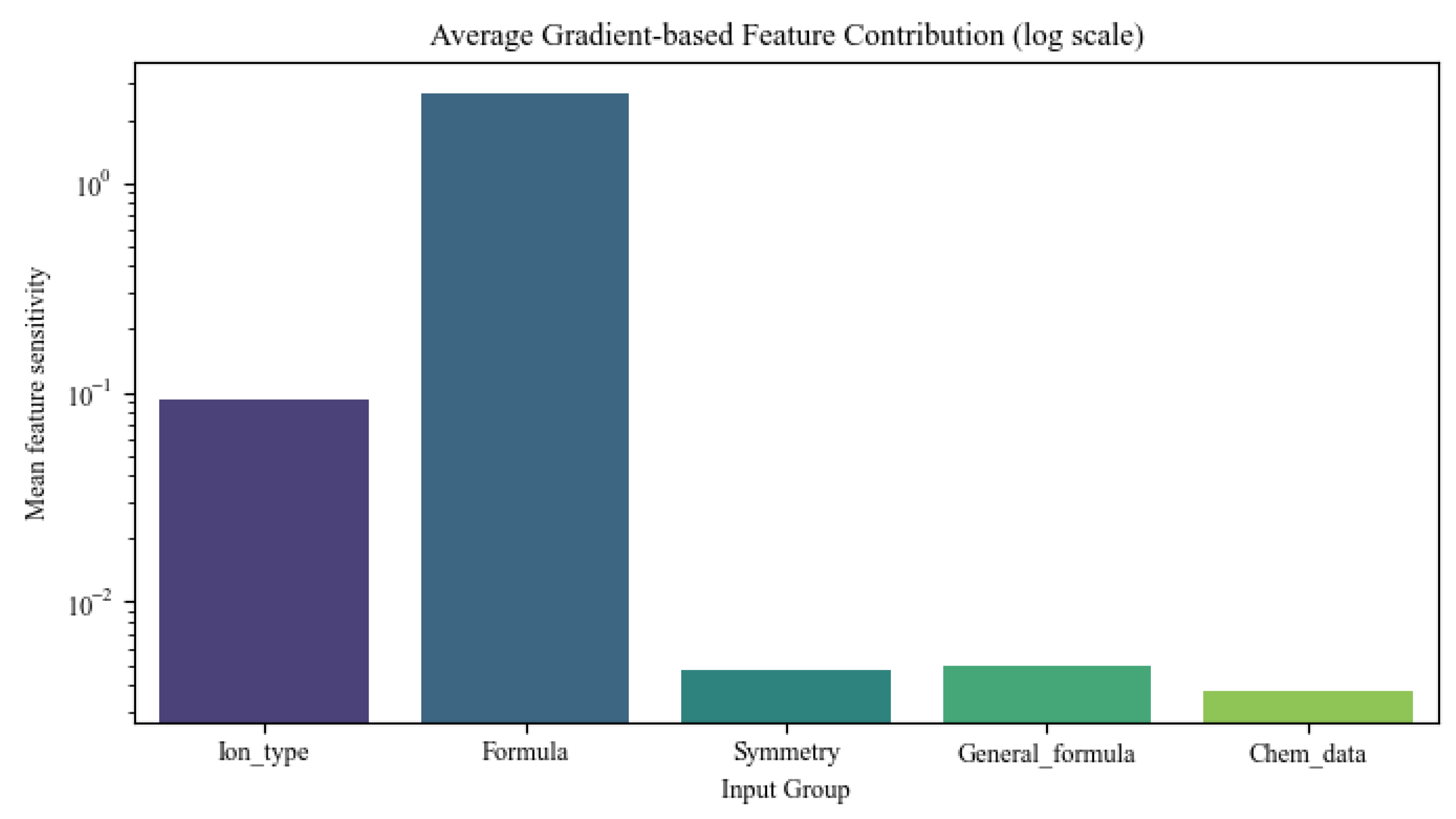
Figure 13 presents the gradient-based feature contribution of five input groups on a logarithmic scale [59]. The vertical axis indicates the mean contribution of each group to the model’s predicted output. The Formula group shows the highest contribution, suggesting that the model relies most heavily on the compositional information of electrode materials. This result reflects the fact that chemical composition is a key determinant of electrochemical capacity and structural stability, while also being partly due to the larger number of features in the Formula group. Next, the Ion type shows a considerable contribution. Although all data correspond to lithium–ion batteries, the insertion and extraction behavior of lithium ions differs depending on the composition and crystal structure of the cathode materials, leading to variations in electrochemical reactivity. In contrast, the Symmetry, General formula, and Chem_data groups exhibit relatively low contributions, indicating that the model uses these as auxiliary information. This suggests that while structural symmetry and basic chemical properties help refine prediction accuracy, their influence is limited compared to compositional and ionic information.

5. Conclusions

In this study, we propose the Classified Branch–CapNet model to accurately predict the gravimetric capacity of lithium–ion battery cathode materials using data collected from the Materials Project. To effectively integrate heterogeneous input data comprising structural and chemical properties, structural data were numerically encoded through physics-based embedding approaches, followed by NMF-based dimensionality reduction to address sparsity issues. Subsequently, each categorical feature was learned through independent pathways and ultimately integrated via late fusion, thereby minimizing the semantic gap between features and enhancing prediction performance. Performance evaluation results demonstrate that the proposed model achieves a mean absolute error (MAE) of 2.441 mAh/g, a root mean square error (RMSE) of 15.236 mAh/g, and a coefficient of determination of 0.961. These results represent prediction error reductions of 56.15%, 71.23%, 73.90%, and 51.1% compared to baseline models of equivalent complexity—namely, the deep neural network (DNN), recurrent neural network (RNN), long short-term memory (LSTM), and encoder-only Transformer architectures, respectively. This indicates that the proposed model effectively learned the influence of structural characteristics on capacity, empirically demonstrating the effectiveness of the parallel architecture that independently learns multi-modal features before integration. Beyond predictive accuracy, computational efficiency analysis reveals that our approach maintains computational advantages comparable to simpler baseline models while demonstrating superior performance. Notably, compared to the encoder-only Transformer model, our method requires only 10% of the computational cost while achieving 50% error reduction, establishing a favorable efficiency-performance trade-off suitable for practical material design applications. The proposed approach effectively addresses the fundamental challenge of feature heterogeneity inherent in concatenation-based fusion commonly used in materials informatics. In conclusion, this study validates that the proposed model constitutes an effective design strategy to enhance prediction performance by effectively fusing high-dimensional, sparse, and heterogeneous battery material data. The methodology is anticipated to serve as a practical AI-driven tool for high-throughput screening and the design of next-generation high-capacity cathode materials, contributing to the acceleration of sustainable energy storage technologies. While the present work leverages the Materials Project database as a robust foundation for model training, future extensions could incorporate experimentally validated synthesis routes to enhance practical applicability. Future studies should investigate the model’s transferability across different cathode chemistries and battery operating conditions, which would establish the Classified Branch–CapNet framework as a versatile tool for both computational and experimental material discovery workflows.

References

1. Yang, Y.; Yang, J.; Wu, X.; Fu, L.; Gao, X.; Xie, X.; Ouyang, Q. Battery pack capacity prediction using deep learning and data compression technique: A method for real-world vehicles. J. Energy Chem. 2025, 106, 553–564. [Google Scholar] [CrossRef]
2. Fu, J.; Song, Z.; Meng, J.; Guo, J.; Yang, K.; Liu, W.; Huan, L. AI-augmented electrochemical model for lithium-ion battery: Recent advances and perspectives. J. Energy Chem. 2025, 113, 1056–1080. [Google Scholar] [CrossRef]
3. Shi, J.-L.; Xiao, D.-D.; Ge, M.; Yu, X.; Chu, Y.; Huang, X.; Zhang, X.-D.; Yin, Y.-X.; Yang, X.-Q.; Guo, Y.-G.; et al. High-capacity cathode material with high voltage for Li-Ion batteries. Adv. Mater. 2018, 30, 1705575. [Google Scholar] [CrossRef]
4. Lyubina, J. Phase transformations and hysteresis in Si-based anode materials. Appl. Phys. Lett. 2021, 118, 090501. [Google Scholar] [CrossRef]
5. Buriak, J.; Toro, C. Positively Highly Cited: Positive Electrode Materials for Li-Ion and Li-Batteries. Chem. Mater. 2018, 30, 559–560. [Google Scholar] [CrossRef]
6. Chakraborty, A.; Kunnikuruvan, S.; Dixit, M.; Major, D. Review of computational studies of NCM cathode materials for Li-Ion batteries. Isr. J. Chem. 2020, 60, 850–862. [Google Scholar] [CrossRef]
7. He, Q.; Yu, B.; Li, Z.; Zhao, Y. Density functional theory for battery materials. Energy Environ. Mater. 2019, 2, 264–279. [Google Scholar] [CrossRef]
8. Jain, A.; Ong, S.P.; Hautier, G.; Chen, W.; Richards, W.D.; Dacek, S.; Cholia, S.; Gunter, D.; Skinner, D.; Ceder, G.; et al. Commentary: The Materials Project: A materials genome approach to accelerating materials innovation. APL Mater. 2013, 1, 011002. [Google Scholar] [CrossRef]
9. Kirklin, S.; Saal, J.E.; Meredig, B.; Thompson, A.; Doak, J.W.; Aykol, M.; Rühl, S.; Wolverton, C. The Open Quantum Materials Database (OQMD): Assessing the accuracy of DFT formation energies. NPJ Comput. Mater. 2015, 1, 15010. [Google Scholar] [CrossRef]
10. Draxl, C.; Scheffler, M. The NOMAD laboratory: From data sharing to artificial intelligence. J. Phys. Mater. 2019, 2, 036001. [Google Scholar] [CrossRef]
11. Curtarolo, S.; Setyawan, W.; Hart, G.L.W.; Jahnatek, M.; Chepulskii, R.V.; Taylor, R.H.; Wang, S.; Xue, J.; Yang, K.; Levy, O.; et al. AFLOW: An automatic framework for high-throughput materials discovery. Comput. Mater. Sci. 2012, 58, 218–226. [Google Scholar] [CrossRef]
12. Shi, X.; Zhou, L.; Huang, Y.; Wu, C.; Wu, Y.; Li, J.; Hong, Z. Machine learning assisted screening of binary alloys for metal-based anode materials. J. Energy Chem. 2025, 104, 62–68. [Google Scholar] [CrossRef]
13. Sawant, V.; Deshmukh, R.; Awati, C. Machine learning techniques for prediction of capacitance and remaining useful life of supercapacitors: A comprehensive review. J. Energy Chem. 2023, 77, 438–451. [Google Scholar] [CrossRef]
14. Manna, S.; Roy, D.; Das, S.; Pathak, B. Capacity prediction of K-ion batteries: A machine learning based approach for high throughput screening of electrode materials. Mater. Adv. 2022, 3, 7833–7845. [Google Scholar] [CrossRef]
15. Zhang, Z.; Wang, Y.; Li, S.; Li, S.; Chen, M. Interpretable Machine Learning Prediction of Voltage and Specific Capacity for Electrode Materials. Adv. Theory Simul. 2024, 7, 2400227. [Google Scholar] [CrossRef]
16. Ma, B.; Zhang, L.; Wang, W.; Yu, H.; Yang, X.; Chen, S.; Wang, H.; Liu, X. Application of deep learning for informatics aided design of electrode materials in metal-ion batteries. Green Energy Environ. 2024, 9, 877–889. [Google Scholar] [CrossRef]
17. Zhou, L.; Yao, A.; Wu, Y.; Hu, Z.; Huang, Y.; Hong, Z. Machine learning assisted prediction of cathode materials for Zn-ion batteries. Adv. Theory Simul. 2021, 4, 2100196. [Google Scholar] [CrossRef]
18. Wang, S.; Ji, Y.; Liu, J.; Liu, Z.; Zhang, X.; Guo, Y.; Lin, J.; Tao, J.; Kasemchainan, J.; Jiang, Y.; et al. Integrating crystal structure and numerical data for predictive models of lithium-ion battery materials: A modified crystal graph convolutional neural networks approach. J. Energy Storage 2024, 80, 110220. [Google Scholar] [CrossRef]
19. Das, K.; Goyal, P.; Lee, S.; Bhattacharjee, S.; Ganguly, N. Crysmmnet: Multimodal representation for crystal property prediction. In Proceedings of the UAI’23: Conference on Uncertainty in Artificial Intelligence, Pittsburgh, PA, USA, 31 July–4 August 2023. [Google Scholar]
20. Liu, C.; Neale, Z.; Cao, G. Understanding electrochemical potentials of cathode materials in rechargeable batteries. Mater. Today 2016, 19, 109–123. [Google Scholar] [CrossRef]
21. Du, M.; Huang, K.; Guo, Y.; Xie, Z.; Jiang, H.; Li, C.; Chen, Y. High specific capacity lithium ion battery cathode material prepared by synthesizing vanadate–phosphate glass in reducing atmosphere. J. Power Sources 2019, 424, 91–99. [Google Scholar] [CrossRef]
22. Goodenough, J. Cathode materials: A personal perspective. J. Power Sources 2007, 174, 996–1000. [Google Scholar] [CrossRef]
23. Barua, A.; Ahmed, M.; Begum, S. A systematic literature review on multimodal machine learning: Applications, challenges, gaps and future directions. IEEE Access 2023, 11, 14804–14831. [Google Scholar] [CrossRef]
24. Baltrušaitis, T.; Ahuja, C.; Morency, L. Multimodal machine learning: A survey and taxonomy. IEEE Trans. Pattern Anal. Mach. Intell. 2018, 41, 423–443. [Google Scholar] [CrossRef] [PubMed]
25. Stahlschmidt, S.R.; Ulfenborg, B.; Synnergren, J. Multimodal deep learning for biomedical data fusion: A review. Brief. Bioinform. 2022, 23, bbab569. [Google Scholar] [CrossRef]
26. Zhang, Q.; Wei, Y.; Han, Z.; Fu, H.; Peng, X.; Deng, C.; Hu, Q.; Xu, C.; Wen, J.; Hu, D.; et al. Multimodal Fusion on Low-quality Data: A Comprehensive Survey. arXiv 2024. [Google Scholar] [CrossRef]
27. Lee, D.; Seung, H.S. Algorithms for non-negative matrix factorization. In Proceedings of the 14th International Conference on Neural Information Processing Systems, Denver, CO, USA, 1 January 2000. [Google Scholar]
28. Zou, H.; Xue, L. A selective overview of sparse principal component analysis. Proc. IEEE 2018, 106, 1311–1320. [Google Scholar] [CrossRef]
29. Xu, J.; Zhu, S.; Xu, Z.; Zhu, H. The basic physical properties of Li2MnO3 and LiMn2O4 cathode materials. Comput. Mater. Sci. 2023, 229, 112426. [Google Scholar] [CrossRef]
30. Huang, Y.; Dong, Y.; Lee, J.; Wang, C.; Zhu, Z.; Xue, W.; Li, Y.; Li, J. Lithium manganese spinel cathodes for lithium-ion batteries. Adv. Energy Mater. 2021, 11, 2000997. [Google Scholar] [CrossRef]
31. Hintze, J.L.; Nelson, R.D. Violin plots: A box plot-density trace synergism. Am. Stat. 1998, 52, 181–184. [Google Scholar] [CrossRef]
32. Akaogi, M.; Ishii, T.; Yamaura, K. Post-spinel-type AB2O4 high-pressure phases in geochemistry and materials science. Commun. Chem. 2024, 7, 189. [Google Scholar] [CrossRef]
33. Toyoda, K.; Adachi, H.; Miyata, N.; Hinogami, R.; Orikasa, Y.; Uchimoto, Y. Surface analysis of topmost layer of epitaxial layered oxide thin film: Application to delafossite oxide for oxygen evolution reaction. Surf. Sci. 2018, 668, 93–99. [Google Scholar] [CrossRef]
34. Kong, H.; Wu, J.; Han, Y.; Zhang, Y.; Zhou, N.; Chen, Q.; Sun, W.; Zhou, H.; Peng, L.M. One-dimensional perovskite-based Li-ion battery anodes with high capacity and cycling stability. J. Energy Chem. 2022, 72, 73–80. [Google Scholar] [CrossRef]
35. Kim, U.-H.; Jun, D.-W.; Park, K.-J.; Zhang, Q.; Kaghazchi, P.; Aurbach, D.; Major, D.T.; Goobes, G.; Dixit, M.; Leifer, N.; et al. Pushing the limit of layered transition metal oxide cathodes for high-energy density rechargeable Li ion batteries. Energy Environ. Sci. 2018, 11, 1271–1279. [Google Scholar] [CrossRef]
36. Menon, R.; Nair, S.S.; Srindhya, K.; Kaimal, M.R. Sparsity-based representation for categorical data. In Proceedings of the IEEE Recent Advances in Intelligent Computational Systems (RAICS), Trivandrum, India, 19–21 December 2013; pp. 74–79. [Google Scholar] [CrossRef]
37. Dahouda, M.K.; Joe, I. A deep-learned embedding technique for categorical features encoding. IEEE Access 2021, 9, 114381–114391. [Google Scholar] [CrossRef]
38. Köppen, M. The curse of dimensionality. In Proceedings of the 5th Online World Conference on Soft Computing in Industrial Applications (WSC5), Online, 4–18 September 2000. [Google Scholar]
39. Eggert, J.; Korner, E. Sparse coding and NMF. In Proceedings of the 2004 IEEE International Joint Conference on Neural Networks (IEEE Cat. No. 04CH37541), Budapest, Hungary, 25–29 July 2004; pp. 2529–2533. [Google Scholar] [CrossRef]
40. Mihelcic, M.; Miettinen, P. Finding Rule-Interpretable Non-Negative Data Representation. IEEE Trans. Knowl. Data Eng. 2025, 37, 2538–2549. [Google Scholar] [CrossRef]
41. Holland, S.M. Principal Components Analysis (PCA); Department of Geology, University of Georgia: Athens, GA, USA, 2008. [Google Scholar]
42. Hyvärinen, A. Independent component analysis: Recent advances Philos. Trans. A Math. Phys. Eng. Sci. 2013, 371, 20110534. [Google Scholar] [CrossRef]
43. McInnes, L.; Healy, J.; Melville, J. UMAP: Uniform Manifold Approximation and Projection for Dimension Reduction. arXiv 2018. [Google Scholar] [CrossRef]
44. Maaten, L.; Hinton, G. Visualizing Data using t-SNE. J. Mach. Learn. Res. 2008, 9, 2579–2605. [Google Scholar]
45. Hamamoto, R.; Takasawa, K.; Machino, H.; Kobayashi, K.; Takahashi, S.; Bolatkan, A.; Shinkai, N.; Sakai, A.; Aoyama, R.; Yamada, M.; et al. Application of non-negative matrix factorization in oncology: One approach for establishing precision medicine. Brief. Bioinform. 2022, 23, bbac246. [Google Scholar] [CrossRef] [PubMed]
46. Boutsidis, C.; Gallopoulos, E. SVD based initialization: A head start for nonnegative matrix factorization. Pattern Recognit. 2008, 41, 1350–1362. [Google Scholar] [CrossRef]
47. Srivastava, N.; Salakhutdinov, R. Multimodal learning with deep boltzmann machines. Adv. Neural Inf. Process. 2014, 25, 2949–2980. [Google Scholar]
48. Nikolaou, N.; Salazar, D.; Raviprakash, H.; Gonçalves, M.; Mulla, R.; Burlutskiy, N.; Markuzon, N.; Jacob, E. A machine learning approach for multimodal data fusion for survival prediction in cancer patients. NPJ Precis. Oncol. 2025, 9, 128. [Google Scholar] [CrossRef]
49. Pawłowski, M.; Wróblewska, A.; Sysko, R.S. Effective techniques for multimodal data fusion: A comparative analysis. Sensors 2023, 23, 2381. [Google Scholar] [CrossRef] [PubMed]
50. Sze, V.; Chen, Y.; Yang, T.; Emer, J. Efficient processing of deep neural networks: A tutorial and survey. Proc. IEEE 2017, 105, 2295–2329. [Google Scholar] [CrossRef]
51. Willmott, C.J.; Matsuura, K. Advantages of the mean absolute error (MAE) over the root mean square error (RMSE) in assessing average model performance. Clim. Res. 2005, 30, 79–82. [Google Scholar] [CrossRef]
52. Hodson, T.O. Root mean square error (RMSE) or mean absolute error (MAE)?—Arguments against avoiding RMSE in the literature. Geosci. Model Dev. 2022, 15, 5481–5487. [Google Scholar] [CrossRef]
53. Chicco, D.; Warrens, M.J.; Jurman, G. The coefficient of determination R-squared is more informative than SMAPE, MAE, MAPE, MSE and RMSE in regression analysis evaluation. PeerJ Comput. Sci. 2021, 7, e623. [Google Scholar] [CrossRef]
54. Du, H.; Hui, J.; Zhang, L.; Wang, H. Rational Design of Deep Learning Networks Based on a Fusion Strategy for Improved Material Property Predictions. J. Chem. Theory Comput. 2024, 20, 6756–6771. [Google Scholar] [CrossRef]
55. Ma, W.; Lei, Y.; Wang, X.; Chen, B. Robust state of charge estimation of lithium-ion battery via mixture kernel mean p-power error loss LSTM with heap-based-optimizer. J. Energy Chem. 2023, 80, 768–784. [Google Scholar] [CrossRef]
56. Bilis, E.; Papadimitriou, T.; Diamantaras, K.; Goulianas, K. EXPERT: EXchange Rate Prediction Using Encoder Representation from Transformers. Forecasting 2025, 7, 65. [Google Scholar] [CrossRef]
57. Gadzicki, K.; Khamsehashari, R.; Zetzsche, C. Early vs late fusion in multimodal convolutional neural networks. In Proceeding of the 2020 IEEE 23rd International Conference on Information Fusion (FUSION), Rustenburg, South Africa, 6–9 July 2020; pp. 1–6. [Google Scholar] [CrossRef]
58. Kohavi, R. A Study of Cross-Validation and Bootstrap for Accuracy Estimation and Model Selection. In Proceedings of the International Joint Conference on Artificial Intelligence, San Francisco, CA, USA, 20–25 August 1995; Volume 14, pp. 1137–1145. [Google Scholar]
59. Ancona, M.; Ceolini, E.; Öztireli, C.; Gross, M. Gradient-Based Attribution Methods. In Explainable AI: Interpreting, Explaining and Visualizing Deep Learning; Springer: Cham, Switzerland, 2019; pp. 169–191. [Google Scholar]
Figure 1. Capacity distribution with Li variation/molecular weight ratio. Red lines indicate the mean capacity values for each interval.
Mathematics 13 03730 g001
Figure 2. Boxplot of capacity corresponding to crystal system. Red dashed lines indicate the mean capacity values for each crystal system.
Mathematics 13 03730 g002
Figure 3. Violin Plots of capacity distribution by representative general formulas.
Mathematics 13 03730 g003
Figure 4. Capacity distribution by representative ion types.
Mathematics 13 03730 g004
Figure 5. Total data points and zero counts before and after applying NMF.
Mathematics 13 03730 g005
Figure 6. Statistical distribution of embedded representations by dataset type.
Mathematics 13 03730 g006
Figure 7. KDE plots across data types.
Mathematics 13 03730 g007
Figure 8. The main architecture of the proposed Classified Branch–CapNet.
Mathematics 13 03730 g008
Figure 9. Data pipeline overview: feature preprocessing and dimensionality reduction followed by capacity prediction through the proposed architecture.
Mathematics 13 03730 g009
Figure 10. The trend analysis between the prediction performance and the fold size of the first hidden layer.
Mathematics 13 03730 g010
Figure 11. Performance comparison between the predicted and actual gravimetric capacity values for (a) DNN, (b) RNN, (c) LSTM, (d) Encoder-only Transformer, and (e) the proposed model.
Mathematics 13 03730 g011
Figure 12. Performance comparison using stratified K-fold cross-validation (K = 3).
Mathematics 13 03730 g012
Figure 13. Comparison of gradient-based input feature contribution.
Mathematics 13 03730 g013