Article

Extreme Theory of Functional Connections with Receding Horizon Control for Aerospace Applications

Systems & Industrial Engineering, University of Arizona, Tucson, AZ 85721, USA
*
Author to whom correspondence should be addressed.
Mathematics 2025, 13(22), 3717; https://doi.org/10.3390/math13223717
Submission received: 13 October 2025 / Revised: 5 November 2025 / Accepted: 13 November 2025 / Published: 19 November 2025
(This article belongs to the Special Issue Advances in Numerical Methods for Optimal Control Problems)

Abstract

This paper introduces a novel closed-loop optimal controller that integrates the Extreme Theory of Functional Connections (X-TFC) with receding horizon control (RHC), referred to as X-TFC-RHC. The controller reformulates a sequence of linearized or quasi-linearized optimal control problems into two-point boundary value problems (TPBVPs) using the indirect method of optimal control. X-TFC then solves each TPBVP by approximating the solution with constrained expressions. These expressions consist of radial basis function neural networks (RBFNNs) and terms that satisfy the TPBVP constraints analytically. The RBFNNs are initialized offline using a particle swarm optimizer, which enables X-TFC to solve the TPBVPs efficiently online during each RHC iteration. The effectiveness of X-TFC-RHC is demonstrated through several aerospace guidance applications, which highlight its accuracy and computational efficiency in executing the RHC process. The proposed approach is also compared with state-of-the-art indirect pseudospectral methods and the traditional backward sweep method.

1. Introduction

Since its introduction in the 1970s, receding horizon control (RHC) has contributed significantly to multiple engineering fields [1]. These include aerospace engineering [2,3,4,5], robotics [6], environmental sciences [7], and chemical engineering [8]. RHC is a closed-loop guidance method in which the current control input is determined by solving a finite-horizon, open-loop optimal control problem (OCP) online. Only the initial control input from the computed sequence is implemented during each guidance cycle. For subsequent cycles, the OCP is resolved at the updated system state with the prediction horizon advanced in time. This iterative process continues until the final time is reached. RHC is widely adopted in engineering due to its applicability to diverse systems, its systematic approach to closed-loop control, stability guarantees under certain conditions [9,10], and strong tracking performance [2,11]. For practical implementation, however, the OCP must be solved significantly faster than the duration of the guidance cycle. Therefore, developing efficient and accurate methods for solving finite-horizon, open-loop OCPs remains an active research area addressed in this work.

1.1. Related Work

Trajectory optimization problems involving nonlinear dynamics are typically divided into an offline trajectory planning phase and an online trajectory tracking phase [12]. The offline phase computes a solution to the full nonlinear OCP, yielding a reference trajectory. The online phase can employ RHC based on linearizing the dynamics about the reference. The solution to the RHC problem was traditionally found by formulating a TPBVP via the indirect method and then applying the backward sweep method or transition matrices to solve a Riccati differential equation (RDE) [13]. Unfortunately, both techniques contain critical pitfalls that limit their use for solving the RHC problem in real time [14,15,16,17,18]. For example, the backward sweep method results in time-intensive integration, and the transition matrix approach can involve inverting highly ill-conditioned matrices. Therefore, alternative approaches that alleviate the drawbacks of traditional methods have been proposed.
Lu developed a receding horizon strategy for precision entry guidance of the X-33, transforming the RHC problem into a quadratic programming problem [12]. The Simpson-trapezoid approximation was applied to solve the integral in the performance index, and Euler-type approximations were used for derivatives in the equations of motion [16,17]. This approach enabled analytical solutions for approximate control laws, although deriving higher-order control laws using this method remains complex. While Lu’s method employs the direct method of optimal control to solve the RHC problem, other researchers have adopted indirect methods. Yan et al. demonstrated that linear quadratic OCPs could be addressed by converting linear time-varying equations into discrete linear algebraic equations using the indirect Legendre pseudospectral method (ILPM) [14]. Subsequently, Yan et al. applied this approach to construct an inner feedback loop for a two-degree-of-freedom control system [2]. Their method utilized RHC to minimize deviations from an optimal reference trajectory. Although the methods proposed by Yan et al. [2,14] and Lu [12,17] addressed several limitations of traditional techniques, both approaches assume that deviations from the reference trajectory remain within the bounds of a linear approximation.
Williams addressed large deviations from the reference trajectory by employing an indirect Jacobi pseudospectral method (IJPM) to integrate RHC with quasi-linearization [3]. Quasi-linearization, also known as the Lagrange–Newton method for function spaces [19], extends the region of convergence beyond standard linearization by solving multiple OCPs in succession [20,21]. The procedure begins with a first-order Taylor expansion about a reference trajectory, neglecting higher-order terms to form a linear OCP. After solving this linear OCP, the process is repeated with linearization performed about the most recent solution. Iterations continue until the difference between consecutive OCP solutions becomes negligible or a predefined maximum number of iterations is reached. Performing only one iteration is equivalent to standard linearization and may result in significant inaccuracies if neglected higher-order terms are substantial. Multiple iterations reduce deviations and diminish the influence of higher-order terms. For certain hyperparameters, quasi-linearization has been proven to yield a convergent solution for all polynomial systems [22]. However, integrating RHC with quasi-linearization increases computational runtime, as each RHC step requires an iterative solution of the OCP with updated initial conditions and horizons. Practitioners must balance solution accuracy against computational efficiency by selecting appropriate tolerances or iteration limits to achieve optimal results.
ILPM and IJPM are similar because both utilize Lagrange orthogonal polynomials. Their namesake comes from collocation at Legendre–Gauss–Lobatto (LGL) and Jacobi–Gauss–Lobatto (JGL) points, both of which include the endpoints of the time domain. Even though ILPM and IJPM are capable of handling complex RHC problems that have been linearized (e.g., hypersonic reentry tracking [11]) and have been improved by transforming the TPBVPs into a set of sparse symmetric positive definite linear algebraic equations [23], researchers continued to build on ILPM and IJPM. In truth, ILPM and IJPM inspired other indirect pseudospectral techniques for solving RHC problems [4,5,24], which utilize different collocation points. Yang et al. developed the Linear Gauss Pseudospectral Model Predictive Controller (LGPMPC) for solving a global OCP with hard terminal constraints (e.g., missile terminal guidance) [4]. It was shown that because LGPMPC used Legendre–Gauss (LG) collocation points (i.e., points where the domain boundaries are not included), it avoided singular differentiation matrices for certain initial conditions that ILPM and IJPM could not. The indirect Gauss pseudospectral method (IGPM) was developed in conjunction with RHC for guiding a quadrotor on optimal paths, and it performed better than state-of-the-art control laws (e.g., pure pursuit, nonlinear guidance law, and trajectory shaping) [24]. Another member of the indirect pseudospectral method family, called the indirect Radau pseudospectral method (IRPM), was introduced by Liao et al. [5]. IRPM uses Legendre–Gauss–Radau points (i.e., points where only one end of the domain is included) and, like its IGPM counterpart, has been shown to be quick and accurate enough for real-time use.

1.2. Contributions and Scope of This Work

This study addresses the RHC problem using the recently introduced Extreme Theory of Functional Connections (X-TFC) method [25]. X-TFC is derived from the Theory of Functional Connections (TFC) [26], a functional interpolation framework that identifies all functions satisfying specified linear constraints exactly. TFC achieves this by analytically embedding constraints into closed-form approximations, referred to as constrained expressions. These expressions are formulated in terms of an arbitrary free function g ( τ ) , along with a summation of switching Ω ( τ ) and projection functional ϱ ( τ ) products that enforce the constraints. A general formulation of a constrained expression is
y ( ) ( τ ) = g ( ) ( τ ) + i = 1 N consts Ω i ( ) ( τ ) ϱ i ( τ i ) ,
where the superscript refers to the th derivative with respect to the independent variable τ . Furthermore, N consts refers to the number of constraints associated with the independent variable y, and τ i within the projection functional indicates that the projection function is always computed on the constraint. The summation of products is what satisfies the linear constraints and is described in further detail in Section 4. Examples of linear constraints that can be embedded include point [27], derivative [28], relative [27], integral [29], and combinations of all four. Since the constrained expressions present a closed-form approximation and satisfy linear constraints exactly, they are incredibly efficient at solving differential equations subject to various constraints at both ends of the domain (i.e., TPBVPs) [28,30].
Previous approaches to solving two-point boundary value problems (TPBVPs) with TFC typically employ orthogonal polynomials, such as Legendre or Chebyshev polynomials, as the free function. When a single-layer feedforward neural network (SLFNN) with randomized input weights and biases is used instead, the method is referred to as Extreme Theory of Functional Connections (X-TFC). A radial basis function neural network (RBFNN) represents a specific type of SLFNN, characterized by activation through radial basis functions and the use of centers and shaping parameters in place of input weights and biases. Prior studies have shown that randomizing the input weights and biases in an SLFNN enables accurate solutions to various differential equations, provided a sufficient number of neurons are included [25,31,32]. In this study, an RBFNN with a limited number of neurons (i.e., 10) is utilized to ensure rapid training suitable for integration with RHC. Unfortunately, employing fewer neurons increases the RBFNN’s sensitivity to the selection of centers and shaping parameters. To address this issue, the network parameters are determined offline using a particle swarm optimizer (PSO) [33]. This study is the first to employ an RBFNN as a TFC-based free function and to optimize, rather than randomize, the X-TFC neural network parameters. Regarding other hybrid neural–RHC frameworks, this work differs in that the PSO is only used to train the RBFNN on the first TPBVP in the RHC process.
There is no universally accepted guideline for selecting the free function; the optimal choice is the one that most accurately approximates the solution to the specific TPBVP. Both TFC with orthogonal polynomials and X-TFC with SLFNNs have demonstrated effectiveness in solving a wide range of TPBVPs arising from the indirect method of optimal control [31,32,34,35,36,37,38,39]. Consequently, either approach is suitable for addressing the RHC problem. This study provides a direct comparison of TFC and X-TFC for RHC applications. Regardless of the selected free function and the resulting constrained expression, TFC and X-TFC employ a procedure analogous to indirect pseudospectral methods: the domain is discretized at Gaussian quadrature points, the TPBVP is converted into a system of algebraic differential equations, and the solution is obtained by applying root-finding algorithms to determine the unknown coefficients through least-squares minimization. Unlike indirect pseudospectral methods, TFC-based approaches approximate the dependent variables using constrained expressions that satisfy the constraints analytically and exactly.
The structure of this document is as follows. First, Section 2 briefly goes over other methods that couple PINNs with RHC and how they differ from X-TFC-RHC. Section 3 then formulates the RHC problem with quasi-linearization. Section 4 details the application of X-TFC to the quasi-linearized RHC problem and describes the optimization of RBFNN centers and shaping parameters using a PSO. A general procedure for implementing the PSO-initialized X-TFC to solve the quasi-linearized RHC problem, referred to as X-TFC-RHC, is also presented. Section 5 presents simulation results for three guidance scenarios: spacecraft relative motion in a circular orbit, planar quadrature maneuver tracking, and longitudinal space shuttle reentry tracking. Analyses of these results demonstrate the robustness of the proposed method across diverse scenarios. The manuscript concludes with a discussion of future work in Section 6 and final remarks in Section 7.

2. X-TFC-RHC Distinction from Other PINN-RHC Methods

When coupled with RHC, PINNs are often used as approximators of the system’s dynamics. This is useful because the differential equations that govern the dynamics can be complex, especially in highly nonlinear systems. Approximating differential equations with PINNs reduces computational burden and can extend the applicability of RHC to more real-time scenarios. Unfortunately, PINNs initially only accepted the continuous-time variable as an input. This hindered their effectiveness when coupled with RHC to approximate the dynamics because the initial state and control were needed as network inputs to build a controlled trajectory over an RHC horizon. Furthermore, traditional PINNs can experience significant degradation in their predictions if trained over long intervals. Antonelo et al. rectified these issues by developing one of the first PINN architectures to be readily applied for RHC, which they called Physics-Informed Neural Nets for Control (PINC) [40]. PINC adds the initial state and control into its neural net framework and splits the time horizon into several shorter intervals. It also enables long-range simulation by chaining network predictions together, setting the initial state of the next interval to the last predicted state of the previous interval. PINC was shown to solve differential equations faster than state-of-the-art numerical solution methods, making them appealing for real-time applications.
Li and Liu extended the PINC method by incorporating TFC and an adaptive loss strategy for automated guided vehicle trajectory tracking, which they called LB-TFC-PINN [41]. Unlike PINC, LB-TFC-PINN does not need to train on the initial state because it is embedded into the dynamics via a TFC constrained expression. Nonetheless, both methods still use a data set comprising many potential fixed control actions (and initial states for PINC) over an RHC time horizon to train their PINN networks offline. Their PINN architectures also consist of multiple hidden layers and allow each layer’s weights and biases to vary with the network inputs. Thus, the equations of motion used by the optimization algorithm to calculate the desired control for each RHC guidance cycle are simply approximated by an already trained PINN for both PINC and LB-TFC-PINN. This is a critical difference between X-TFC-RHC, PINC, and LB-TFC-PINN. X-TFC-RHC uses a single-hidden-layer PINN, where only the weights of the single hidden layer are trained offline via a PSO. Those weights correspond to the centers and shaping parameters of the radial basis activation function. Furthermore, these hidden-layer weights are trained only on the first OCP in the RHC process, drastically reducing training time.
Another major distinction between X-TFC-RHC and the aforementioned PINN-RHC methods is that X-TFC-RHC attempts to linearize the dynamics it approximates. Hence, X-TFC-RHC can train the output weights of its single-hidden-layer network in a single iteration, almost instantaneously, assuming the hidden-layer weights are already known. Of course, the hidden-layer weights are already known from the offline PSO training step. Thus, the hidden-layer weights are held constant for each linearized OCP in the RHC process being solved, and the output weights are computed in real time. The output weights in the PINC and LB-TFC-PINN methods are trained offline along with the hidden-layer weights. X-TFC-RHC is very similar to indirect pseudospectral methods because the output weights are computed as the OCP is solved. This is why indirect pseudospectral methods for RHC were given so much emphasis in this manuscript’s introduction.

3. Problem Formulation

The performance index of any successive OCP within the RHC process can be expressed as
J = 1 2 x ( t + T ) x f S f x ( t + T ) x f + 1 2 t t + T [ x ( τ ) x ref ( τ ) Q ( τ ) x ( τ ) x ref ( τ ) + u ( τ ) u ref ( τ ) R ( τ ) u ( τ ) u ref ( τ ) ] d τ ,
where x ( τ ) R n is the actual state vector, x ref ( τ ) R n is the reference state vector, u ( τ ) R m is the vector of actual control inputs, u ref ( τ ) R m is the reference control input, t R is the current time, τ [ t , t + T ] is the time range for which each individual OCP is solved, T is the horizon length, x f = x ( τ = t + T ) R n is the desired terminal state vector at the end of the horizon, S f R n × n is a positive semidefinite terminal weighting matrix, Q ( τ ) R n × n is a positive semidefinite matrix that weights the state residual x ( τ ) x ref ( τ ) , and R ( τ ) R m × m is a positive definite matrix that weights the control residual u ( τ ) u ref ( τ ) . Each OCP involves finding u ( τ ) that minimizes Equation (2) whilst subjected to equations of motion. These equations can be represented as either linear or nonlinear systems, which are often time-varying. A linear time-varying system can be expressed as
x ˙ ( τ ) = A ( τ ) x ( τ ) + B ( τ ) u ( τ ) x ( τ = t ) = x 0 ,
where A ( τ ) R n × n and B ( τ ) R n × m are time-varying matrices, and x 0 = x ( τ = t ) R n is the initial condition. A nonlinear time-varying system is typically written as
x ˙ = f τ , x ( τ ) , u ( τ ) x ( τ = t ) = x 0 ,
where f R n is a vector of nonlinear functions. Each RHC problem, depending on whether the equations of motion are linear or nonlinear, can be written compactly as
min u ( 2 ) s . t . ( 3 ) or ( 4 ) .
When the equations of motion in the RHC problem are nonlinear, they need to be linearized to ensure efficient (i.e., fast and accurate) numerical solutions. Similar to Refs. [3,5], X-TFC-RHC handles situations where the initial deviations are too great for an accurate linear approximation by employing quasi-linearization. In quasi-linearization, the performance index is identical to Equation (2), except that the state and control variables are now with respect to the quasi-linearization procedure’s current iteration x ˜ ( τ ) , u ˜ ( τ ) . Furthermore, the equations of motion are expanded to first order about the quasi-linearization procedure’s previous iteration x ˜ ( τ ) , u ˜ ( τ )  [21,22]. Any trajectory can be used to initialize the procedure, but this study uses the reference trajectory. The solution to the original nonlinear RHC problem can be computed by successively solving the quasi-linearized OCPs. Applying quasi-linearization, Equation (2) becomes
J ˜ = 1 2 x ˜ ( t + T ) x f S f x ˜ ( t + T ) x f + 1 2 t t + T [ x ˜ ( τ ) x ref ( τ ) Q ( τ ) x ˜ ( τ ) x ref ( τ ) + u ˜ ( τ ) u ref ( τ ) R ( τ ) u ˜ ( τ ) u ref ( τ ) ] d τ .
Furthermore, Equation (4) becomes
x ˜ ˙ = A ˜ ( τ ) x ˜ ( τ ) + B ˜ ( τ ) u ˜ ( τ ) + w ˜ ( τ ) x ˜ ( τ = t ) = x ˜ 0 ,
where
A ˜ ( τ ) = f τ , x ( τ ) , u ( τ ) x | x ˜ ( τ ) , u ˜ ( τ )
B ˜ ( τ ) = f τ , x ( τ ) , u ( τ ) u | x ˜ ( τ ) , u ˜ ( τ )
and
w ˜ ( τ ) = f τ , x ˜ ( τ ) , u ˜ ( τ ) A ˜ ( τ ) x ˜ ( τ ) B ˜ ( τ ) u ˜ ( τ ) .
The OCPs that must be solved successively can then be expressed as
min u ˜ ( 6 ) s . t . ( 7 ) .
Following the indirect method, the TPBVP necessary for solving Equation (8) is acquired by first deriving the Hamiltonian, which is given by
H ( τ ) = 1 2 [ x ˜ ( τ ) x ref ( τ ) Q ( τ ) x ˜ ( τ ) x ref ( τ ) + u ˜ ( τ ) u ref ( τ ) R ( τ ) u ˜ ( τ ) u ref ( τ ) ] + λ ˜ ( τ ) A ˜ ( τ ) x ˜ ( τ ) + B ˜ ( τ ) u ˜ ( τ ) + w ˜ ( τ ) ,
where λ ˜ ( τ ) R n is the costate vector for the current iteration. By minimizing the Hamiltonian with respect to the current control, its optimal value can be found in terms of the costates as follows:
H ( τ ) u ˜ ( τ ) = 0 u ˜ ( τ ) = u ref ( τ ) R 1 ( τ ) B ˜ ( τ ) λ ˜ ( τ ) .
Plugging Equation (10) into Equation (9), the costate differential equations (i.e., necessary conditions for optimality) and their terminal conditions can then be obtained from the calculus of variations,
λ ˜ ˙ ( τ ) = Q ( τ ) x ˜ ( τ ) x ref ( τ ) A ˜ ( τ ) λ ˜ ( τ ) λ ˜ ( τ = t + T ) = S f x ˜ ( t + T ) x f .
We can then write the linear TPBVP in matrix form by combining Equations (11) and (7) with Equation (10),
x ˜ ˙ ( τ ) λ ˜ ˙ ( τ ) = A ˜ ( τ ) B ˜ ( τ ) R 1 ( τ ) B ˜ ( τ ) Q ( τ ) A ˜ ( τ ) x ˜ ( τ ) λ ˜ ( τ ) + B ˜ ( τ ) u ref ( τ ) + w ˜ ( τ ) Q ( τ ) x ref ( τ ) x ˜ ( τ = t ) = x ˜ 0 λ ˜ ( τ = t + T ) = S f x ˜ ( t + T ) x f .

4. Method

Whether solving Equation (12) with an indirect pseudospectral method or X-TFC, the first step involves rewriting the differential equations such that all of their terms are on one side of the equals sign, such that
0 = x ˜ ˙ ( τ ) λ ˜ ˙ ( τ ) + A ˜ ( τ ) B ˜ ( τ ) R 1 ( τ ) B ˜ ( τ ) Q ( τ ) A ˜ ( τ ) x ˜ ( τ ) λ ˜ ( τ ) + B ˜ ( τ ) u ref ( τ ) w ˜ ( τ ) Q ( τ ) x ref ( τ ) .
The ILPM, IJPM, IRPM, and ILGM then approximate the state and costate variables as Lagrange polynomials. On the other hand, X-TFC approximates the states and costates with constrained expressions that analytically embed the constraints. Thus, they will be exactly satisfied, unlike when most indirect pseudospectral methods are performed (we acknowledge the IGPM shown in Ref. [24] solves for the constraints via Gauss quadrature and not with least squares like the other indirect pseudospectral methods. Gauss quadrature is exact for the RHC problem, but it still treats the constraints differently than X-TFC because they are not incorporated into a constrained expression. Section 5 provides a comparison of the two methods). Several works provide general outlines for how to define TFC-based constrained expressions and then use them to solve general TPBVPs [26,31,42]. For the reader’s convenience, the definitions of constrained expressions for a general TPBVP are shown in Appendix A. In this section, how constrained expressions are defined based on the constraints in Equation (12) and how they are subsequently used to solve Equation (12) is given.
Since the initial condition x ˜ ( t ) = x ˜ 0 is a point constraint only in terms of x ˜ ( τ ) , it will be embedded with the constrained expression that represents x ˜ ( τ ) . Notice that the terminal condition λ ˜ ( t + T ) = S f x ˜ ( t + T ) x f does not consist of only one dependent variable, unlike the initial condition. The terminal condition is a relative constraint in terms of both x ˜ ( τ ) and λ ˜ ( τ ) . Thus, there is a choice to be made. Should the terminal constraint be embedded in the constrained expression that represents x ˜ ( τ ) or λ ˜ ( τ ) ? Both options are valid, but each constrained expression will only contain one constraint if λ ˜ ( τ ) is selected. This greatly simplifies the derivation of the constrained expressions, as is about to be shown.
The general constrained expression shown in Equation (1) is only for approximating a scalar. Since the dependent variables within Equation (12) are expressed as vectors, so too must their constrained expressions. Thus, the constrained expressions that approximate x ˜ ( τ ) and λ ˜ ( τ ) are
x ˜ ( τ ) g x ( τ ) + Ω x ( τ ) ϱ x ( t )
and
λ ˜ ( τ ) g λ ( τ ) + Ω λ ( τ ) ϱ λ ( t + T ) .
g x ( τ ) R n and g λ ( τ ) R n are free function vectors for the state and costate, respectively; Ω x ( τ ) R n and Ω λ ( τ ) R n are switching function vectors for the state and costate, respectively; ϱ x ( t ) R n and ϱ λ ( t + T ) R n are projection functional vectors for the state and costate, respectively. Note that only one switching and projection function vector is present in both constrained expressions. This correlates to the number of constraints in each differential equation within Equation (12), which is one. There would be two switching and projection function vectors in Equation (14) and zero in Equation (15) had the relative terminal constraint been embedded into the constrained expression for x ˜ ( τ ) . Conveniently, Ω x ( τ ) = Ω λ ( τ ) = 1 when there is only one constraint (see Appendix A for the reason). Furthermore, the projection functional for point constraints is simply the difference between the constraint value and the free function where the constraint occurs (see Ref. [26]),
ϱ x ( t ) = x ˜ 0 g x ( t ) .
For relative constraints, the projection functional is equal to each term in the constraint brought to one side of the equals sign and each dependent variable written out as their respective free function at where the constraint occurs (see Ref. [26]),
ϱ λ ( t + T ) = S f g x ( t + T ) x f g λ ( t + T ) .
For clarity, let us see what happens to the constrained expressions when the independent values on the constraints are input, along with the switching and projection functionals:
x ˜ ( t ) g x ( t ) + x ˜ 0 g x ( t ) = x ˜ 0 λ ˜ ( t + T ) g λ ( t ) + S f g x ( t + T ) x f g λ ( t + T ) = S f g x ( t + T ) x f .
Clearly, the free functions associated with the dependent variable that the constrained expression is approximating cancel out, and all that is left is the expression for the constraint, effectively embedding the constraint.
RBFNNs can be used for the free functions within Equations (14) and (15). As their name suggests, RBFNNs rely on radial basis functions (RBFs),
φ ( τ , c ) = φ ( τ c 2 ) ,
where c is the RBF center and · 2 denotes the L2-norm (i.e., Euclidean distance). RBFNNs are preferred in this work for their easily adjustable smoothness and powerful convergence properties [43]. Any function satisfying Equation (18) is called an RBF, which can be infinitely smooth or piecewise smooth. Infinitely smooth RBFs are also called global RBFs and are often used when approximating smooth functions. On the contrary, piecewise RBFs are preferred for approximating nonsmooth functions. We use a global RBF in this work because the RHC solution is globally smooth. More specifically, a Gaussian RBF (GRBF) is used,
φ ( τ , c , ϵ ) = exp ϵ 2 τ c 2 ,
where ϵ is a shaping parameter that controls the width of the GRBF. GRBFs make up the hidden-layer kernels in our RBFNN. Thus, the free function can be expressed as
g ( · ) ( τ ) = k = 1 L β ( · ) k φ ( τ , c k , ϵ k ) = φ ( τ , c 1 , ϵ 1 ) φ ( τ , c L , ϵ L ) β ( · ) 1 β ( · ) L = φ ( τ ) β ( · ) .
β ( · ) k R L are the output weights that connect the kth hidden neuron/GRBF to the output solution; c k R L and ϵ k R L are the centers and shaping parameters associated with the kth hidden neuron/GRBF, respectively; L is the total number hidden neurons/GRBFs in the RBFNN. Notice that the free function in Equation (19) is in index notation where the subscript ( · ) is simply a placeholder. Any element of the state or costate can be substituted for it to show what constrained expression the free function is part of (e.g., ( · ) = x i i = { 1 , 2 , , n } or ( · ) = λ i i = { 1 , 2 , , n } ). Thus, each free function is a unique RBFNN, meaning there are 2 n RBFNNs. Another important observation from Equation (19) is that each RBFNN uses the same centers and shaping parameters.
Since X-TFC computes the unknown solution x ˜ ( τ ) , λ ˜ ( τ ) via the ELM algorithm, c k and ϵ k can be randomized and not tuned during training [44]. Therefore, they are known parameters. The unknown coefficients associated with the kth hidden neuron/GRBF within each RBFNN β ( · ) k R L are what must be computed. Using the aforementioned observations about Equation (19), the free function vector for the state and costate can be written as
g x ( τ ) = V ( τ ) Ξ x
and
g λ ( τ ) = V ( τ ) Ξ λ ,
where
Ξ x = β x 1 β x 2 β x n R n L
Ξ λ = β λ 1 β λ 2 β λ n R n L
and
V ( τ ) = φ ( τ ) 0 0 0 0 φ ( τ ) 0 0 0 0 φ ( τ ) 0 0 0 0 φ ( τ ) R n × n L .
To have better training performance, it is convenient to map the independent variable τ [ τ 0 , τ f ] = [ t , t + T ] in the domain z [ z 0 , z f ] = [ 1 , + 1 ] . This is accomplished using the following linear transformation:
z = z 0 + b ( τ t ) τ = t + 1 b ( z z 0 ) ,
where b is the mapping coefficient
b = z f z 0 t ( t + T ) = 2 T .
By the derivative chain rule, the th derivative of the free function is
d g ( · ) ( τ ) d τ = b d ϕ ( z ) d z β ( · ) .
Plugging Equations (16), (17), (20), and (21) into Equations (14) and (15); applying Ω x ( τ ) = Ω λ ( τ ) = 1 ; performing a change of basis to the z domain; and employing Equation (22) then yields the constrained expressions and their derivatives:
x ˜ ( τ ) = x ˜ ( z ) V ( z ) V ( z 0 ) Ξ x + x ˜ 0
λ ˜ ( τ ) = λ ˜ ( z ) V ( z ) V ( z f ) Ξ λ + S f V ( z f ) Ξ x x f
d x ˜ ( τ ) d τ = 2 T d x ˜ ( z ) d z 2 T D ( z ) Ξ x
d λ ˜ ( τ ) d τ = 2 T d λ ˜ ( z ) d z 2 T D ( z ) Ξ λ ,
where
D ( z ) = φ ( z ) d z 0 0 0 0 φ ( z ) d z 0 0 0 0 φ ( z ) d z 0 0 0 0 φ ( z ) d z R n × n L .
Substituting the Equations (23)–(26) into Equation (13) allows an unconstrained system whose solution analytically satisfies the initial and terminal constraints to be formed. The z domain must be discretized (i.e., collocated) to solve this system numerically. Equally spaced points may be chosen, but a quadrature scheme like the LGL points is heavily preferred to avoid the Runge phenomenon [45]. Equation (13) with the constrained expressions plugged in at each discretization point z d d = { 0 , 1 , , N } can then be expressed in block matrix notation as
E ^ F ^ G ^ H ^ Ξ x Ξ λ = O ^ Ξ = J ^ K ^ = P ^ ,
where E ^ , F ^ , G ^ , H ^ R N + 1 n × L n , whose ( d , j ) th blocks are n × n L matrices of the following form:
E ^ d j = 2 T D ( z d ) A ˜ ( z d ) V ( z d ) V ( z 0 ) + B ˜ ( z d ) R 1 ( z d ) B ˜ ( z d ) S f V ( z f ) F ^ d j = B ˜ ( z d ) R 1 ( z d ) B ˜ ( z d ) V ( z d ) V ( z f ) G ^ d j = Q ( z d ) V ( z d ) V ( z 0 ) + A ˜ ( z d ) S f V ( z f ) H ^ d j = 2 T D ( z d ) + A ˜ ( z d ) V ( z d ) V ( z f ) .
Furthermore, J ^ and K ^ R N + 1 n , as well as their k th blocks, are n × 1 vectors of the following form:
J ^ d = A ˜ ( z d ) x ˜ 0 + B ˜ ( z d ) u ref d + w ˜ ( z d ) + B ˜ ( z d ) R 1 ( z d ) B ˜ ( z d ) S f x f K ^ d = Q ( z d ) x ref d x ˜ 0 + A ˜ ( z d ) S f x f .
The coefficients that make up Ξ x and Ξ λ in Equation (27) can easily be solved for via linear least squares,
Ξ = O ^ O ^ 1 O ^ P ^ .
When N + 1 = L , like in this study, linear least squares does not have to be performed to solve for Ξ . A simple inversion does the trick,
Ξ = O ^ 1 P ^ .
Plugging the computed Ξ x and Ξ λ values into the constrained expressions and mapping back to the τ domain then gives the x ˜ ( τ ) , λ ˜ ( τ ) solution at the discretized points. The solution for the control at the discretized points can be calculated with Equation (10). Lastly, the accuracy of the X-TFC method can be determined by moving each term in Equation (27) to one side of the equal sign,
L = O ^ Ξ P ^ .
The L R 2 ( N + 1 ) n parameter is the loss, and the closer its Euclidean norm is to 0, the more accurate the solution is.

4.1. Radial Basis Function Neural Network Initialization

For the inversion in Equation (28) to be performed quickly, the number of neurons in the RBFNN needs to be small while still being capable of approximating the RHC solution accurately. If the centers and shaping parameters within the RBFNN are randomized, then there is a very likely chance that the RBFNN will fail to approximate each OCP solution well over its horizon. For example, Figure 1a shows a possible collection of GRBFs with their centers and shaping parameters randomized, along with 5 LGL collocation points. All the GRBFs are equal to 0 at the horizon’s beginning, where two collocation points exist. Thus, Figure 1a clearly shows that the GRBFs may not activate for all the collocation points when the centers and shaping parameters are randomized, which would cause the RBFNN to fail in approximating the solution accurately. Alternatively, Figure 1b shows a collection of GRBFs with their centers aligned on the collocation points and their widths fixed small with large constant shaping parameters. In this case, the RBFNN will better approximate the solution on the collocation points. However, the RBFNN will not generalize well because there are regions of the domain where all the GRBFs equal 0. A collection of GRBFs that would generalize much better than those in Figure 1a,b are those with smaller shaping parameters, resulting in larger widths, as shown in Figure 1c. In Figure 1c, all GRBFs affect the output of the RBFNN over the entire domain. This is not always the best approach because GRBFs centered in highly nonlinear regions of the domain may adversely affect the solution at discretization points farther away.
An RBFNN that generalizes well is necessary to solve most regression problems. Engineers and scientists often desire good approximations at points not included in the data. However, this study is not interested in interpolating with the constrained expressions from X-TFC. Only the solution at the beginning of the horizon, which is discretized with the LGL points, is desired to obtain the control action for the current guidance cycle. Thus, the RHC problem merely requires a good approximation at the discretization points so that the solution at the very beginning of each OCP’s horizon is accurate. Using this logic, selecting the GRBFs like in Figure 1b seems reasonable. Nonetheless, Fornberg and Zuev have shown that allowing the shaping parameters to vary for each GRBF leads to more accurate approximations [45]. Indeed, new methods for selecting the ideal set of RBFNN network parameters are actively sought. Many clustering [46,47,48] and evolutionary techniques [49,50,51] have been proposed.
Inspired by Ref. [52], a PSO is used to find the ideal set of shaping parameters with the centers placed at the collocated LGL points in this work. Many different variants of the original PSO algorithm have been developed since its inception [53]. To maintain a suitable trade-off between exploration and exploitation, the PSO variant with a constriction factor K [54] is used in the X-TFC-RHC process, along with a damping coefficient ς . Only the first OCP in the RHC scheme is repeatedly solved with X-TFC in the PSO to obtain the ideal shaping parameters. It is shown in Section 5 that optimizing the shaping parameters from only the first OCP yields accurate results for the OCPs solved at later horizons. Although the authors did not encounter applications in which changing the initialized centers and shaping parameters was necessary, more complex problems may require adaptively modifying the centers and shaping parameters for different OCPs in the receding horizon sequence. If that is the case, an adaptive residual subsampling procedure like that shown in Ref. [55] could be used. Other questions the reader might have may include the following: Why not use a PSO to optimize the centers as well? Why use the PSO with a constriction factor from Ref. [54] instead of a different PSO modification, or an entirely different method to initialize? Indeed, these are valid questions and worth future study. Regardless, determining the best procedure for initializing the X-TFC RBFNN is outside the scope of this paper.
The objective of any PSO algorithm is to find the global minimum (or maximum) of a cost function by incorporating the experience of a swarm of particles. Each particle represents potential inputs to the cost function. In this work, the cost function is the X-TFC solver used to solve the first OCP, as stated earlier. The output of this cost function is not the state or control trajectory. Instead, the cost function’s output is the Euclidean distance of Equation (29) because L 2 is what needs to be minimized to acquire an accurate solution. We will refer to this cost function as Cost ( N + 1 = L , T , ϵ ) . The main inputs that are preselected and held constant include the number of collocation points set equal to the number of neurons N + 1 = L and the horizon length T. Since the centers of the RBFNNs are fixed to the collocated LGL points, the only inputs left to optimize for with the PSO are the shaping parameters ϵ R L . Thus, the PSO’s search space is an L-dimensional space (i.e., each particle has L dimensions). It is worth noting that the PSO must be rerun to find a new ϵ if T, L, or the collocation points are changed.
The shaping parameter position and velocity for an lth particle can be expressed as ϵ l = ϵ l 1 ϵ l 2 , , ϵ l L and ϵ l = ϵ l 1 , ϵ l 2 , , ϵ l L , respectively, where l = { 1 , 2 , , N p } . All L shaping parameters for each particle are first uniformly randomized between a minimum and maximum value, ϵ min and ϵ max . This randomization is represented with the function Unifrnd ( ϵ min , ϵ max , L ) , where L indicates that there are a total of L randomized shaping parameters for each particle. Each particle’s position and velocity vector are updated from iteration a to the next, a + 1 , all the way to a max via
ϵ l ( a + 1 ) = ϵ l ( a ) + ϵ l ( a )
and
ϵ l ( a + 1 ) = K [ ϵ l ( a ) + ζ 1 r 1 p l ϵ l ( a ) + ζ 2 r 2 p best ϵ l ( a ) ] .
The reader should be aware that ( a ) in Equations (30) and (31) are used to represent the computation of the shaping parameters at the PSO’s a iteration instead of representing that the shaping parameters are a function of the PSO’s a iteration. The constriction factor is given as
K = 2 2 ζ 1 ζ 2 ζ 1 + ζ 2 2 4 ζ 1 + ζ 2 ,
where ζ 1 + ζ 2 > 4 . The parameters ζ 1 and ζ 2 are constants that weight the best previous position of the lth particle, p l , and the best previous position of all particles, p best , respectively. The parameters r 1 and r 2 are two independent random values uniformly distributed on [ 0 , 1 ] . The p l and p best parameters are found by using ϵ l ( a ) as inputs to Cost and storing the results. Note that K is multiplied by a parameter ζ < 1 , but still near 1, during each a iteration, such that velocities are more likely to decrease on each iteration. Once a = a max , a way to tell that the PSO has found a suitable minimum for L 2 is when ϵ ( a = a max ) is low relative to ϵ ( a = 1 ) and p best has not changed for several iterations. For the reader’s convenience, a pseudocode of the PSO used and all its hyperparameters are given in Algorithm 1 and Table 1, respectively.

4.2. X-TFC-RHC Procedure

Until now, the proposed method may seem complex due to the multiple iterations required across several steps. Here, we hope to alleviate any confusion about how X-TFC-RHC functions. The X-TFC solver is first initialized with a PSO. The PSO is computationally expensive, but this is not a factor because it is executed offline. The initialized X-TFC solver can then be employed online to solve successive OCPs for the RHC problem, thereby stabilizing the control system along the reference. If the problem is nonlinear, each OCP can be solved iteratively using quasi-linearization to maintain the linear approximation. The X-TFC-RHC approach is similar to the methods presented in Refs. [3,5], with the exception that X-TFC is used and initialized with a PSO. To clarify, an algorithm flowchart of the X-TFC-RHC procedure is given in Appendix B, and its summary is as follows:
Algorithm 1 PSO with X-TFC
  1:
procedure  PSO ( L , T , ζ 1 , ζ 2 , ς , ϵ min , ϵ max , ϵ min , ϵ max , a max , N p )
  2:
     K ( 32 )
  3:
    for  a = 1 , , a max  do
  4:
         K K · ς
  5:
        if  a = 1  then
  6:
           for  l = 1 , , N p  do
  7:
                ϵ l ( a ) Unifrnd ( ϵ min , ϵ max , L , 1 )
  8:
                ϵ l ( a ) Unifrnd ( ϵ min , ϵ max , L , 1 )
  9:
                p l ϵ l ( a )
10:
           end for
11:
            p best min 1 l N p Cost ( L , T , p i )
12:
        end if
13:
        for  l = 1 , , N p  do
14:
            ϵ l ( a + 1 ) ( 31 )
15:
            ϵ l ( a + 1 ) ( 30 )
16:
           for  k = 1 , , L  do
17:
               if  ϵ l k < ϵ min  then
18:
                    ϵ l k = ϵ min
19:
               else if  ϵ l k > ϵ max  then
20:
                    ϵ l k = ϵ max
21:
               else if  ϵ l k < ϵ min  then
22:
                    ϵ l k = ϵ min
23:
               else if  ϵ l k > ϵ max  then
24:
                    ϵ l k = ϵ max
25:
               end if
26:
           end for
27:
           if  Cost ( L , T , ϵ l ( a ) ) < Cost ( L , T , p l )  then
28:
                p l ϵ l ( a )
29:
           end if
30:
        end for
31:
         p best min 1 l N p Cost ( L , T , p l )
32:
    end for
33:
    return  p best
34:
end procedure
  • Set the initial time τ 0 , final time τ f , guidance cycle t gc , time horizon length T, and an equivalent number of collocation points and neuorns N + 1 = L .
  • Initialize the X-TFC solver offline by having the RBFNN centers align with the collocation points and optimize for the shaping parameters. The optimization procedure is carried out with the PSO shown in Algorithm 1 and with the hyperparameters given in Table 1. The cost function the PSO is minimizing involves carrying out the X-TFC process for the first OCP in the RHC process where the dynamics are linearized along a reference trajectory x ref , u ref over the interval τ [ t 0 , t 0 + T ] . The final cost to be minimized is the Euclidean norm of Equation (29).
  • With the X-TFC solver initialized, online control can begin by linearizing the equations of motion about the reference trajectory over the interval τ [ t , t + T ] to form Equation (12). Note that this step is redundant for the very first iteration in the RHC process because it was also carried out during the PSO step for t = τ 0 .
  • Solve a sequence of TPBVPs for the nonlinear case (quasi-linearization) or a single TPBVP for the linear case:
    (a)
    Solve Equation (12) with the initialized X-TFC solver. The outcome will be the unknown coefficients Ξ of the RBFNN.
    (b)
    Plug the Ξ coefficients into Equations (23) and (24) to get the state and costates over the horizon. Then plug the states and costates into Equation (10) to get the control over the horizon.
    (c)
    If Equation (5) is nonlinear, then linearize the equations of motion over the solution just obtained to form Equation (12) again. If Equation (5) is linear, ignore this step.
    (d)
    When Equation (5) is nonlinear, repeat steps (a), (b), and (c) until the Euclidean norm of the change in state variable x ˜ x ˜ 2 is below some tolerance ε quasi or maximum number of iterations κ max is reached. Remember that x ˜ is the previous quasi-linearized state solution. Move on to Step 5 if Equation (5) is linear or the quasi-linearization stopping criteria is reached.
  • Apply the optimal control action at the current time t, which is obtained from the converged trajectory during Step 4 for the nonlinear system or the immediate result for the linear system, while integrating the dynamics for one guidance cycle t g c . The entire RHC process starting at Step 3 is then repeated with t = t + t gc until t + T = τ f , the end of the reference.
Lastly, if κ max = 1 or x ˜ x ˜ 2 < ε quasi on the first iteration of Step 3, then just standard linearization should be performed on the nonlinear RHC problem (i.e., one iteration only). If x ˜ x ˜ 2 > ε quasi , then more quasi-linearization iterations should be run so that the actual trajectory is stabilized.

4.3. A Note on Stability

We do not explicitly prove the stability of the X-TFC-RHC controller in this manuscript. Instead, we rely on the numerous works by other researchers that guarantee stability for nonlinear RHC methods under certain conditions [9], which include the following: constraining the final state to origin/reference trajectory [56,57], incorporating contractive constraints [58], and including an approprate terminal cost in the performance index [59,60]. Furthermore, it is well known that RHC without final constraints and open-loop OCPs solved sequentially requires a sufficiently long horizon to ensure stability and constraint satisfaction [61]. That is precisely how we assume X-TFC-RHC’s stability in this work. We merely select an adequate time horizon through trial and error. A more formal proof of X-TFC-RHC’s stability is left for future work.

5. Applications

This section applies X-TFC-RHC to several guidance problems: circular orbit relative motion, planar quadrotor tracking, and longitudinal space shuttle reentry guidance. Whether linear, nonlinear, time-varying, or time-invariant, each problem is solved successfully with the proposed method. The applications shown were chosen to highlight a particular aspect of X-TFC-RHC’s performance. For example, the spacecraft relative motion in a circular orbit application showcases the computational speed of the method and how varying the time horizon length affects the result. How varying the number of collocation points and neurons affects the results is shown as well. The planar quadrotor application demonstrates that the quasi-linearization aspect of X-TFC-RHC stabilizes along the reference and compares well with the state-of-the-art indirect pseudospectral methods. Lastly, the longitudinal space shuttle reentry guidance application exemplifies X-TFC-RHC’s robustness through a Monte Carlo simulation in which the initial state varies, and a time comparison with the traditional backward sweep method is provided. X-TFC-RHC, which solved all these problems, was coded in MATLAB® R2021a and run on an Intel Core i7-9700 CPU with 64 GB of RAM.

5.1. Spacecraft Relative Motion in a Circular Orbit

The circular orbit relative motion problem involves a deputy satellite rendezvousing with a target point in a circular orbit around the Earth, which is referred to as the chief. The relative acceleration between the deputy and the chief can be described by the Clohessy–Wiltshire (CW) equations, which make use of a Local Vertical–Local Horizontal (LVLH) coordinate frame centered on the chief [35]. These equations can be written as
x ˙ ( τ ) = 0 0 0 1 0 0 0 0 0 0 1 0 0 0 0 0 0 1 3 ω 2 0 0 0 2 ω 0 0 0 0 2 ω 0 0 0 0 ω 2 0 0 0 x ( τ ) + 0 0 0 0 0 0 0 0 0 1 0 0 0 1 0 0 0 1 u ( τ ) ,
where ω is the angular velocity of the chief,
ω = μ / a sm 3 .
The μ parameter represents Earth’s gravitational parameter and a sm is the semimajor axis of the chief’s circular orbit. Also, the state is made up of the relative 3-dimensional positional and velocity components, x ( τ ) = [ r 1 ( τ ) , r 2 ( τ ) , r 3 ( τ ) , v 1 ( τ ) , v 2 ( τ ) , v 3 ( τ ) ] . Likewise, the control is the deputy’s relative commanded acceleration, u ( τ ) = [ u 1 ( τ ) , u 2 ( τ ) , u 3 ( τ ) ] . Lastly, the performance index is identical to Equation (2).
For this application, μ = 3.986004418 × 10 14 m 3 / s 2 and a sm = 7500 × 10 3 m . To improve numerical performance, the position, velocity, commanded acceleration, and time were normalized as follows:
t = t / ω r = r / a sm v = v / ( a sm ω ) a c = a c / ( a sm ω 2 ) .
The RHC problem shown in Equation (5) was formed by having the unnormalized initial state’s position and velocity vectors set to r 0 = [ 7047 , 5136 , 5013 ] m and v 0 = [ 2.4 , 13.7 , 4.08 ] m/s. To rendezvous with the chief, the deputy had to reach the state x f = 0 and hold there. To accomplish this, the weight matrices used were Q = diag ( 1 × 10 4 , 1 × 10 4 , 1 × 10 4 , 1 × 10 2 , 1 × 10 2 , 1 × 10 2 ) , R = I 3 , and S f = I 6 . Note that diag ( · ) represents a square diagonal matrix based on the content of ( · ) and I ( · ) is a square identity matrix of size ( · ) . The unnormalized guidance cycle applied was t gc = 10 s, the final time was τ f = 2000 s, the collocation scheme used was LGL, and the number of collocation points and neurons were N + 1 = L = 10 . Lastly, the reference state and control were x ref = 0 and u ref = 0 for every moment in time, respectively.
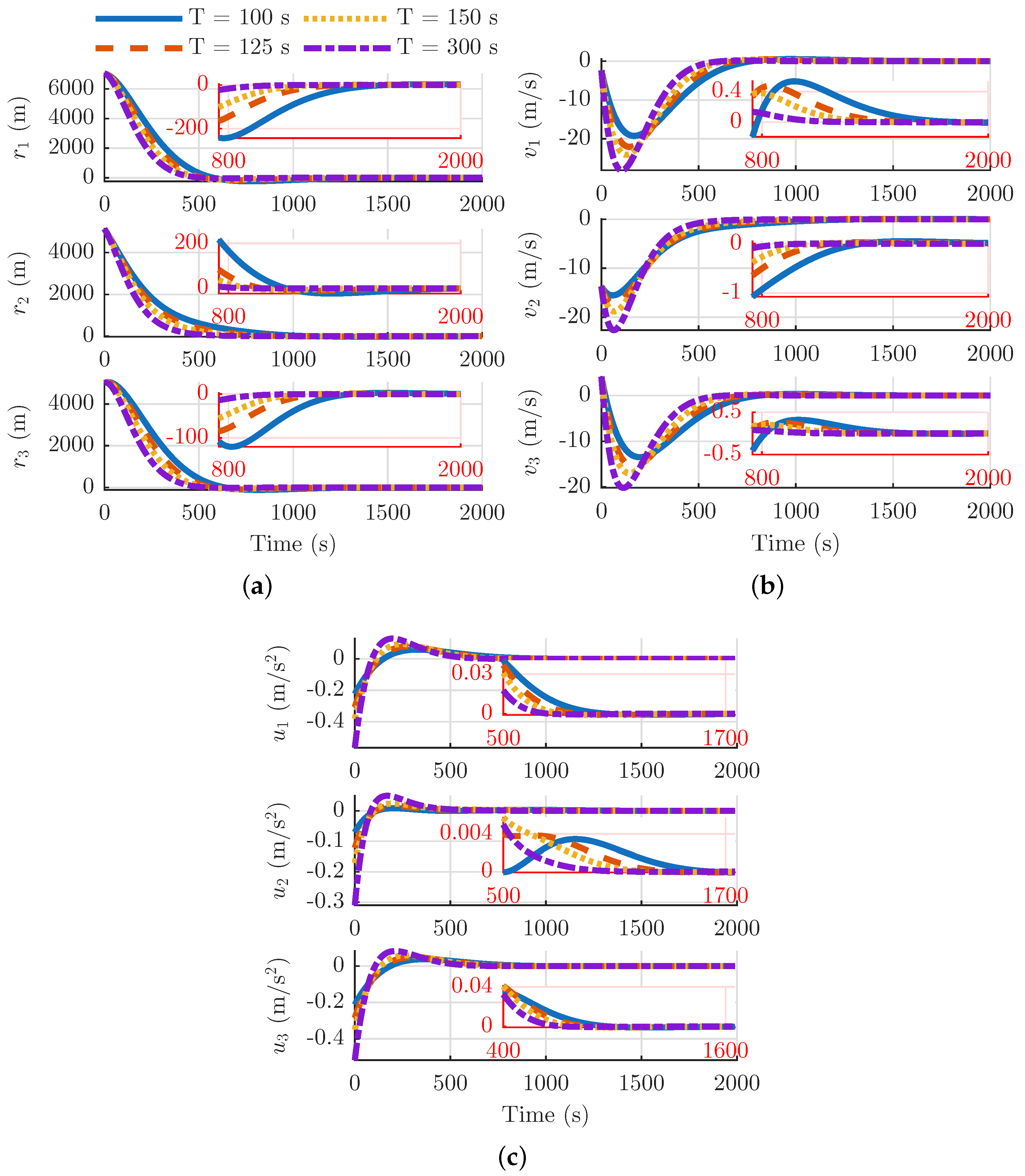
A sensitivity study was conducted by varying the time horizon T. The results of the proposed X-TFC-RHC method when T = { 100 , 125 , 150 , 300 } s are shown in Figure 2. By observing the figures, one can see that the X-TFC-RHC method successfully guides the deputy to the chief. However, how quickly the method guides the satellite to the final destination depends on T. As T increases, the settling time decreases and vice versa. The settling time decreases when T is larger because of the resulting lack of overshoot. When T is smaller, the overshoot is too great for the controller to stabilize the deputy at the chief as quickly as when T is large. Different T values than those shown were also tested. What was found was that if T was smaller than 65 s, then the deputy could not settle at the chief within τ f because the overshoot was too great. When T = τ f , the controller was still able to stabilize quickly. The reader should be aware that, depending on the problem, large T values will require more collocation points and neurons to approximate the solution of the RHC problem accurately. Since the equations of relative motion for this problem were linear and N + 1 = L = 10 , X-TFC-RHC continued to effectively guide the satellite to the chief as T increased.
Next, simulations were performed with N + 1 = L varying (while still equal to each other) and T held constant to analyze the computational efficiency of the X-TFC-RHC controller. The results of this study are shown in Table 2. As N + 1 = L increases, the maximum and average computation time of X-TFC for solving each successive OCP increases. This is the case because O ^ and P ^ from Equation (27) become larger as N + 1 = L increase. Hence, the inversion step in Equation (28) takes longer. When N + 1 = L is held constant and T increases, the average computation time is steady. Thus, to run the X-TFC-RHC controller as quickly as possible, one should use the fewest number of collocation points and neurons so that each OCP solution can be approximated accurately over the chosen time horizon. Obviously, the maximum computation time should be significantly lower than the guidance cycle, which is the case for this application.
From this application, it can be concluded that the computation efficiency of the proposed optimal control law depends on the number of collocation points and neurons. The gains of the optimal control law are mainly affected by the length of the time horizon. For this application, the centers of each RBFNN were placed at the LGL points and the shaping parameters were optimized before each simulation using a PSO. How long the PSO took to initialize the RBFNN for each case in Table 2 can be calculated by t cal_ave × a max × N p , where a max and N p are given in Table 1. Even when each iteration of the RHC process ran the fastest, initializing the PSO still took about a minute. This proves why the PSO must initialize the RBFNN offline. The following application compares the difference in solutions for when the X-TFC-RHC process is carried out as described and when the centers and shaping parameters are randomized.

5.2. Planar Quadrotor Tracking

The simplified planar quadrotor model is well established and has been used to generate trajectories of isolated maneuvers in several studies [62,63,64]. The state associated with this model is as follows: x ( τ ) and z ( τ ) are the position of the quadrotor’s center of mass in the inertial ( x , z ) -plane; θ ( τ ) represents the attitude of the quadrator by being the angle about its body axis normal to the inertial ( x , z ) -plane; x ˙ ( τ ) and z ˙ ( τ ) are the velocity of the quadrotor’s center of mass in the inertial ( x , z ) -plane; and θ ˙ ( τ ) is the angular rate of the quadrotor’s body axis normal to the ( x , z ) -plane. The quadrotor’s control inputs are made up of its collective thrust divided by its mass, u 1 ( τ ) = T ( τ ) / m , and its torque divided by its inertia about the body axis normal to the inertial ( x 1 , x 2 ) -plane, u 2 ( τ ) = τ ^ ( τ ) / J ^ . See Ref. [65] for more details about the planar quadrotor model. For our simulations, m = 0.5 kg and J ^ = 3 × 10 3 kg · m 2 . Using the state x ˙ ( τ ) = [ x ( τ ) , z ( τ ) , θ ( τ ) , x ˙ ( τ ) , z ˙ ( τ ) , θ ˙ ( τ ) ] and control u ˙ ( τ ) = [ u 1 ( τ ) , u 2 ( τ ) ] , the equations of motion for the planar model can be written as
x ˙ ( τ ) = x ˙ ( τ ) z ˙ ( τ ) θ ˙ ( τ ) u 1 ( τ ) sin θ ( τ ) u 1 ( τ ) cos θ ( τ ) g u 2 ( τ ) ,
where g is the gravitational acceleration.
A point-to-point reference trajectory was computed for the X-TFC-RHC controller to track. The maneuver simply brings the quadrotor from one position to the other with zero velocity and attitude imposed at both ends of the trajectory. The maneuver’s reference trajectory was computed using GPOPs-II [66] with the performance index
J ref = 1 2 0 τ f u u d τ
and constraints on the controls defined as
FoS 1 T max m u 1 FoS 2 T min m ,
where T min = 1 N and T max = 12 N are the minimum and maximum thrust, respectively. The FoS 1 = 3 and FoS 2 = 0.8 parameters are factors of safety associated with the minimum and maximum thrust. These safety factors were necessary to ensure that the control of the tracked trajectory remained within the thrust bounds. Furthermore, an absolute maximum constraint on the absolute torque was applied, τ ^ max = 0.2 N·m, but it posed significantly less risk of violation than the thrust constraint. The maneuver started with the x ( τ 0 ) = [ 0 , 0 , 0 , 0 , 0 , 0 , ] initial condition and had the final condition x ( τ f ) = [ 20 , 40 , 0 , 0 , 0 , 0 , ] .
The equations of motion shown in Equation (33) are nonlinear. Thus, tracking a planar quadrotor reference maneuver trajectory requires approximating the equations of motion at discrete points along the reference trajectory using the quasi-linearization method. The nonzero elements of the Jacobian matrices A ˜ R 6 × 6 and B ˜ R 6 × 2 in Equation (12) can be computed as A ˜ 14 = 1 , A ˜ 25 = 1 , A ˜ 36 = 1 , A ˜ 43 = u 1 cos x 3 , A ˜ 53 = u 1 sin x 3 , B ˜ 41 = sin x 3 , B ˜ 51 = cos x 3 , and B ˜ 62 = 1 . Since the Jacobians are based on a time-varying trajectory, they are functions of time.
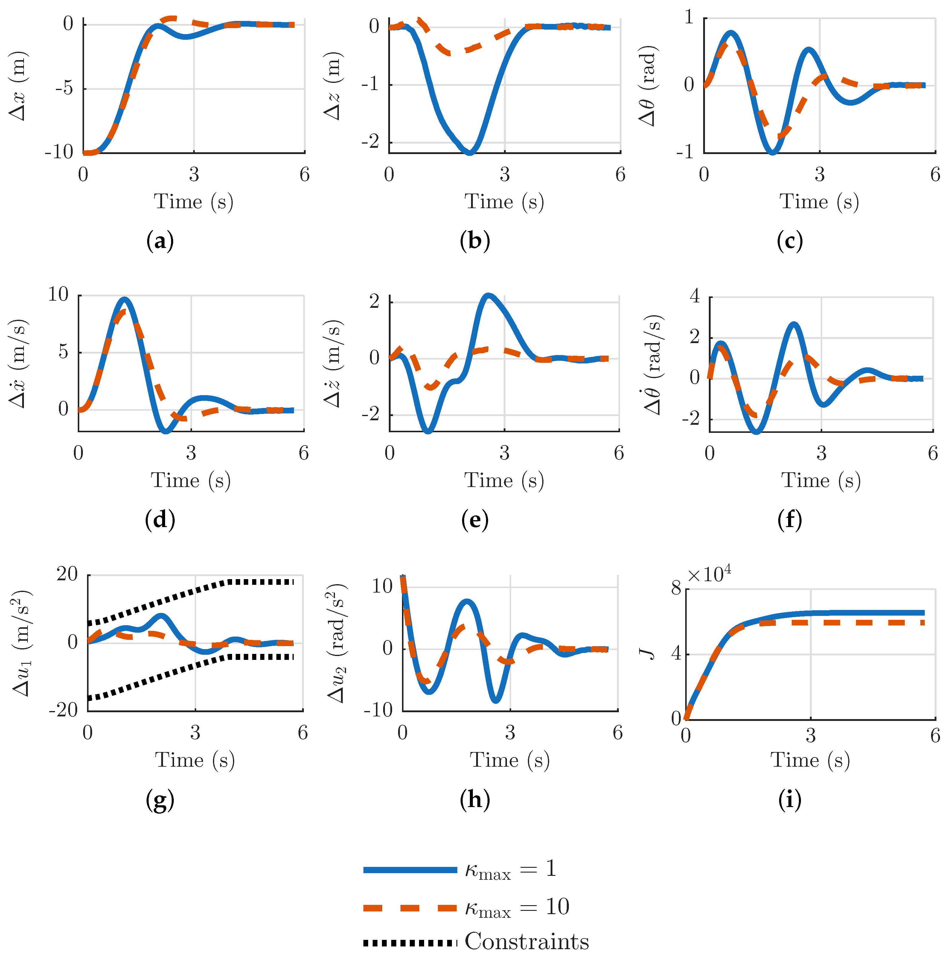
We tracked the point-to-point maneuver with an initial-state perturbation of Δ x = [ 10 , 0 , 0 , 0 , 0 , 0 ] from the reference. The weight matrices were set to S f = 0 , Q = diag ( 500 , 500 , 500 , 10 , 10 , 20 ) , and R = diag ( 700 exp ( 1.5 t ) , 300 exp ( 1.5 t ) ) . The chosen R matrix heavily weighted the control deviation from the reference at the beginning of the trajectory, causing the control constraint to be enforced. The guidance cycle was set to t gc = 0.01 s, the time horizon was T = 3 s, the final time of the tracking trajectory was equivalent to that of the reference trajectory ( τ f 5.9 s), the collocation scheme used was LGL, and the amount of collcations were equal to the amount of neurons in the RBFNN ( N + 1 = L = 10 ). Since quasi-linearization was performed to approximate the dynamics, the tolerance was set to ε quasi = 1 × 10 6 and the maximum amount of iterations varied between κ max = 1 and κ max = 10 . Figure 3 shows the tracking results.
Figure 3 shows an inherent benefit when more iterations are performed. The X-TFC-RHC controller causes the quadrotor to stabilize on the reference trajectory faster and with less overshoot when 10 quasi-linearization iterations are performed, compared to just 1. Furthermore, the accumulated cost of the final trajectory when κ max = 10 is lower than when κ max = 1 . This provides evidence of the trajectory’s global optimality as more quasi-linearization iterations are performed. Although the difference between X-TFC’s solution when solving the quasi-linearized RHC problems is visually apparent, the convergence capability of the X-TFC-RHC process with quasi-linearization needs to be analyzed. Thus, several metrics for analyzing the difference between the X-TFC-RHC quasi-linearization result and some highly accurate solution ( · ) * were composed:
e ^ J = J ˜ J ˜ 2 e ^ x = x ˜ x ˜ 2 e ^ λ = λ ˜ λ ˜ 2 e ^ u = u ˜ u ˜ 2 .
Typically ( · ) would be an exact analytical solution. However, no analytical solution exists for the planar quadrotor problem. Thus, the highly accurate solution used for this scenario was the X-TFC quasi-linearization result with κ max = , but with ε quasi = 10 10 . Using the metrics given in Equation (35), a comparison was made between X-TFC’s quasi-linearization results when ε quasi varied and κ max was held constant. The results of this comparison are given in Table 3. As expected, the quasi-linearization results approach the highly accurate solution as the prescribed tolerance decreases. As the simulation progresses and the trajectory approaches a steady state, fewer iterations are needed to reach the prescribed tolerance.
We carried out another quasi-linearization test where ϵ quasi = 1 × 10 10 was held constant, and κ max varied. The metrics used for this test are shown below in Equation (36):
e ¯ J = J ˜ κ max J ˜ κ max 1 2 e ¯ x = max ( x ˜ κ max x ˜ κ max 1 2 , z ˜ κ max z ˜ κ max 1 2 ,       θ ˜ κ max θ ˜ κ max 1 2 , x ˜ ˙ κ max x ˜ ˙ κ max 1 2 ,       z ˜ ˙ κ max z ˜ ˙ κ max 1 2 , θ ˜ ˙ κ max θ ˜ ˙ κ max 1 2 ) e ¯ λ = max ( λ x κ max λ ˜ x κ max 1 2 , λ ˜ z κ max λ ˜ z κ max 1 2 ,       λ ˜ θ κ max λ ˜ θ κ max 1 2 , λ ˜ x ˙ 1 κ max λ ˜ x ˙ 1 κ max 1 2 ,       λ ˜ z ˙ 1 κ max λ ˜ z ˙ 1 κ max 1 2 , λ ˜ θ ˙ 1 κ max λ ˜ θ ˙ 1 κ max 1 2 ) e ¯ u = max u ˜ 1 κ max u ˜ 1 κ max 1 2 , u ˜ 2 κ max u ˜ 2 κ max 1 2 .
where ( · ) κ max indicates the result at the maximum iteration and ( · ) κ max 1 is the result for the iteration prior. Table 4 shows these measured metrics for the cases where the maximum iteration was varied. As shown, the X-TFC-RHC controller coupled with quasi-linearization converges nicely in 20 iterations.
Decreasing ε quasi and increasing κ max both ensure the actual trajectory stabilizes at the reference because the previous iteration’s trajectory solution is used for linearizing the dynamics, which is closer to the reference’s linear approximation. However, more quasi-linearization iterations lead to slower computation times. Thus, ε quasi and κ max must be carefully selected to balance out convergence with computation time. X-TFC-RHC is clearly able to track the maneuver and the control stays within the constraints due to the implementation of the factor of safety in Equation (34).
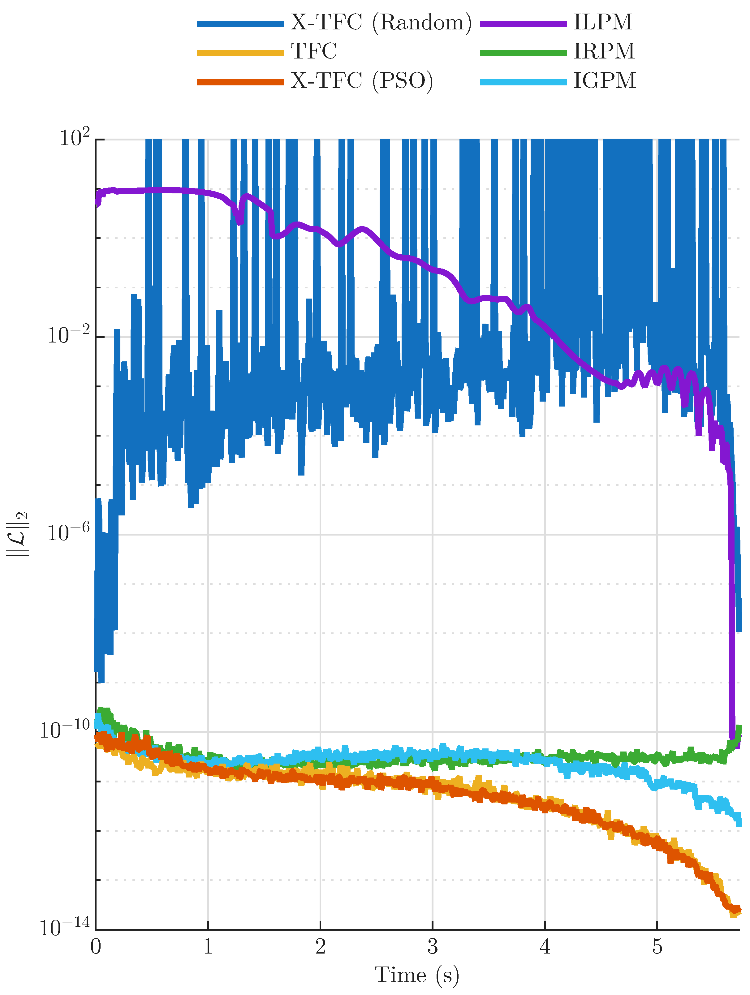
The results shown for this application so far involved initializing the RBFNN’s shaping parameters with the PSO and holding the centers at the collocation points. How do these results compare when other TFC-based setups and various indirect pseudospectral methods are performed? To answer this question, the same planar quadrotor tracking RHC problem used to generate Figure 3 with κ max = 10 and ε quasi = 10 10 was solved. However, several different TPBVP solvers were used: X-TFC with RBFNNs as the free function, along with their centers and shaping parameters randomized, X-TFC (Random); the X-TFC-RHC method proposed in this paper, X-TFC (PSO); TFC with Chebyshev orthogonal polynomials as the free function; the ILPM [14]; the IRPM [5]; the IGPM [24]. Each method used the same LGL collocation scheme with N + 1 = 10 and an identical time horizon, T = 3 s. The L 2 of each successive OCP was measured for each method. The results are shown in Figure 4. The lower the L 2 values throughout the trajectory, the more accurate the solution.
One can see that TFC with Chebyshev orthogonal polynomial free functions is more accurate than the indirect pseudospectral methods, which use Lagrange polynomials. Interestingly, the ILPM method is the least accurate. This is likely because the ILPM differentiation matrix has a much higher condition number than those of the IRPM and IGPM for this problem. X-TFC with the RBFNN’s centers and shaping parameters randomized is the next least accurate out of all the methods. When the centers are placed at the collocation points and the shaping parameters are optimized with a PSO, X-TFC appears to be just as accurate as TFC.
Lastly, note that a comparison between the computational speed of the various techniques was not needed because they all belong to the family of collocation methods. Collocation methods involve representing the solution as a linear combination of polynomials, whose unknown coefficients are then solved with the Gauss–Newton algorithm in this study. To keep the accuracy comparison fair, the same number of collocation points and number of neurons (basis functions for TFC and indirect pseudospectral methods) were the same, with N + 1 = L = 10 . Hence, the runtime of each method for solving one RHC OCP with one quasi-linearization iteration was approximately 1.2 × 10 3 s, as shown in Table 2.

5.3. Longitudinal Space Shuttle Reentry Tracking

This application involved tracking the longitudinal components of a space shuttle reentry trajectory. The full equations of motion are as follows [67]:
r ˙ ( τ ) = V ( τ ) sin ( γ ( τ ) ) θ ˙ ( τ ) = V ( τ ) cos ( γ ( τ ) ) cos ( ψ ( τ ) ) r ( τ ) cos ( θ ( τ ) ) ϕ ˙ ( τ ) = V ( τ ) cos ( γ ( τ ) ) sin ( ψ ( τ ) ) r ( τ )
V ˙ ( τ ) = D ( τ ) g ( τ ) sin ( γ ( τ ) )
γ ˙ ( τ ) = L ( τ ) cos ( σ ( τ ) ) V ( τ ) g ( τ ) cos ( γ ( τ ) ) V ( τ ) + V ( τ ) r ( τ ) cos ( γ ( τ ) ) ψ ˙ ( τ ) = L ( τ ) sin ( σ ( τ ) ) V ( τ ) cos ( γ ( τ ) ) V ( τ ) r ( τ ) cos ( γ ( τ ) ) cos ( ψ ( τ ) ) tan ( ϕ ( τ ) ) .
where the state is the radial r ( τ ) , longitude θ ( τ ) , latitude ϕ ( τ ) , speed V ( τ ) , flight path angle γ ( τ ) , and the heading angle ψ ( τ ) . The gravitational acceleration is given as g ( τ ) = μ / r ( τ ) 2 (see the first test case for the definition of μ ). The lift and drag accelerations are
D ( τ ) = ρ ( τ ) V ( τ ) 2 S area C D ( τ ) 2 m
and
L ( τ ) = ρ ( τ ) V ( τ ) 2 S area C L ( τ ) 2 m ,
where the shuttle’s reference area and mass are S area = 249.9092   m 2 and m = 92,709 kg, respectively. Furthermore, ρ ( τ ) is the atmospheric density model given as ρ ( τ ) = ρ 0 exp ( r ( τ ) R e ) / h s , where ρ 0 = 1.225 kg / m 3 is the sea level atmospheric density, R e = 6,371,004 m is the Earth’s radius, and h s = 7254.2 m is the density scale height. The lift coefficient C L and drag coefficient C D are given as
C L ( τ ) = C L 0 + C L 1 α ( τ )
and
C D ( τ ) = C D 0 C D 1 α + C D 2 α ( τ ) 2 ,
where C L 0 = 0.2070 , C L 1 = 1.6756 , C D 0 = 0.0785 , C D 1 = 0.3529 , and C D 2 = 2.0400 . The shuttle’s control inputs are the bank angle σ and the angle of attack α . Lastly, the shuttle’s path constraints consist of the heating rate Q ˙ , dynamic pressure q, and normal load n. The equations for each are
Q ˙ ( τ ) = k Q ρ ( τ ) V ( τ ) 3.15 Q ˙ max = 2 × 10 6 W / m 2
q ( τ ) = 1 2 ρ ( τ ) V ( τ ) 2 q max = 2 × 10 4 Pa
n ( τ ) = L ( τ ) 2 + D ( τ ) 2 / g n max = 2.5 ,
where k Q = 1.65 × 10 4 is the vehicle’s heat flux transmission coefficient.
The initial state conditions for generating the reference were r 0 = R e + 79,250 m, θ 0 = 0 deg, ϕ 0 = 0 deg, V 0 = 7800 m/s, γ 0 = 1 deg ψ 0 = 90 deg; and the terminal state constraints were r f = R e + 24,384 m, V f = 762 m/s, and γ f = 5 deg. The reference trajectory was calculated with GPOPs-II in the same manner as performed for the previous application. The only difference was that the performance index for computing the shuttle reference was
J ref = ϕ ( τ f ) .
Hence, the reference is generated by solving an OCP for the final maximum latitude. Once the reference trajectory was computed, the longitudinal space shuttle reentry guidance (tracking) problem was formulated by only incorporating Equations (37)–(39) into the RHC problem, which was then solved with X-TFC-RHC. The nonzero elements of the Jacobian matrices A ˜ R 3 × 3 and B ˜ R 3 × 2 in Equation (12) are as follows:
A ˜ 12 = V ( τ ) sin γ ( τ ) A ˜ 13 = V ( τ ) cos γ ( τ ) A ˜ 21 = ρ ( τ ) S ref C D ( τ ) V ( τ ) 2 2 h s m + 2 g ( τ ) sin γ ( τ ) r ( τ ) A ˜ 22 = ρ ( τ ) S ref C D ( τ ) V ( τ ) 2 m A ˜ 23 = g ( τ ) cos γ ( τ ) A ˜ 31 = ρ ( τ ) S ref C L ( τ ) V ( τ ) cos σ ( τ ) 2 m h s V ( τ ) cos γ ( τ ) r ( τ ) 2 + 2 g ( τ ) cos γ ( τ ) V ( τ ) r ( τ ) A ˜ 32 = ρ ( τ ) S ref cos σ ( τ ) 2 m + g ( τ ) V ( τ ) 2 + 1 r ( τ ) cos γ ( τ ) A ˜ 33 = g ( τ ) V ( τ ) + V ( τ ) r ( τ ) sin γ ( τ ) B ˜ 22 = ρ ( τ ) S ref V ( τ ) 2 C D 1 + 2 C D 2 α ( τ ) 2 m B ˜ 31 = ρ ( τ ) S ref V ( τ ) C L ( τ ) sin σ ( τ ) 2 m B ˜ 32 = ρ ( τ ) S ref V ( τ ) C L 1 cos σ ( τ ) 2 m .
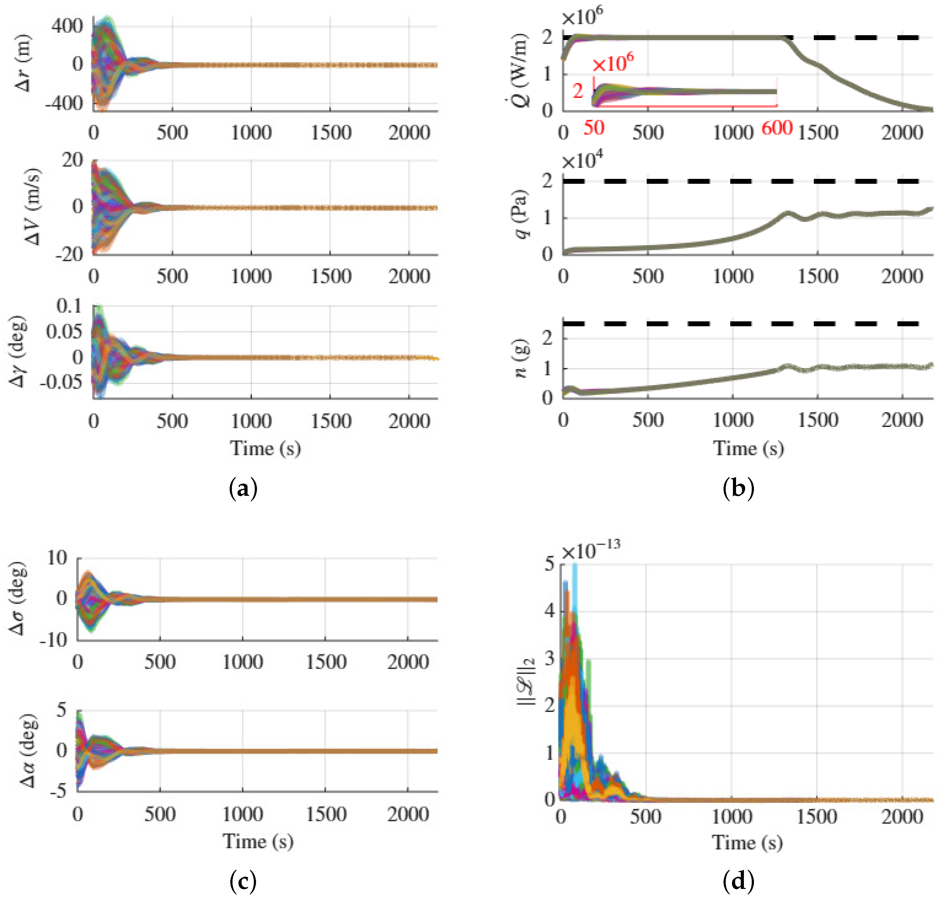
500 Monte Carlo simulations where the initial state perturbations from the reference varied uniformly were performed to analyze the robustness of the X-TFC-RHC method. The uniform bounds of each longitudinal state were Δ r = [ 300 , 300 ] m, Δ V = [ 20 , 20 ] m/s, and Δ γ = [ 0.05 , 0.05 ] deg. For each closed-loop guidance simulation, t g c = 1 s, Q = diag ( 1.2 × 10 6 , 190 , 0 ) , R = diag ( 0.01 , 0.04 ) , S f = 0 ( 3 ) , T = 200 s, an LGL collocation scheme is used, and N + 1 = L = 10 . Furthermore, quasi-linearization with κ max = 1 was used to approximate the dynamics (i.e., linearization). By observing the Monte Carlo results shown in Figure 5, one can see that the X-TFC-RHC controller can stabilize the shuttle on the reference trajectory for every simulation. The reference is tracked close enough that the heat rate constraint is barely violated near the beginning of the trajectory. Incorporating a factor of safety similar to that used in the previous application to generate the reference can alleviate this violation. Nevertheless, the L 2 values for all Monte Carlo trajectories are under 3 × 10 13 , further showing the accuracy and reliability of the proposed method.
An experiment comparing the computation speed of X-TFC with that of the backward sweep method was conducted. Unlike the previous experiment, Monte Carlo simulations were not performed. Instead, the initial-state deviation remained constant at the previously shown maximum bounds. The backward sweep method was performed with the Runge–Kutta 4 algorithm to iterate the RDE. An algorithm with an adaptive step size, like Runge–Kutta 45, could have been used, but it was desired to align the integral step size (these time steps varied across the domain such that they were equal to the time increments between each LGL collocation point used in X-TFC) with the collocation points of X-TFC in order to keep the experiment fair. An explicit integration algorithm was not used because its adaptive step sizes are iterative and inherently lead to higher computational costs. Lastly, the horizon length used each time the backward sweep method was applied in the RHC process was identical to that of X-TFC.
Table 5 shows the computation time statistics for solving each OCP in the RHC process. Interestingly, the backward sweep method with Runge–Kutta 4 failed to solve the RDE unless the time step was small enough to discretize the domain into 31 LGL points. This makes sense because the RDE tends to be numerically unstable [68]. On the other hand, X-TFC could easily solve the OCPs with only 10 collocation points. Table 5 shows that X-TFC with 10 and 31 collocation points is both quicker than the backward sweep method with Runge–Kutta 4 on average.

6. Comment on Future Work

The results and analysis presented in this study show that X-TFC-RHC, with an initialized RBFNN, is worthy of consideration for real-time guidance. The same can even be said for X-TFC’s parent, TFC with a Chebyshev free function. TFC may even be more suitable because it does not require initialization. Regardless, this work is only a precursor of what is to come. Functional interpolation-based methods, such as TFC and X-TFC, can likely handle RHC problems with steady-state error. Steady-state error is traditionally handled by augmenting the state error to the system so that integral action is incorporated [69]. TFC-based methods could eliminate steady-state error completely by adding an integral constraint to the constrained expression instead. Steady-state error could also be handled by using a reinforcement learning approach to determine the ideal hyperparameters of the RBFNN throughout all phases of the trajectory, similar to Ref. [70].
This study could also be improved through online retraining of the RBFNN centers and shaping parameters. In the X-TFC-RHC process shown, the RBFNN hyperparameters are trained only on the first RHC OCP, which was feasible for the test cases presented. Nonetheless, it may be necessary to update RBFNN hyperparameters for OCPs later in the RHC process if the dynamics of the time-varying systems change dramatically. This can easily be achieved in an RHC iteration by first solving the RHC TPBVP, Equation (12), as shown in Section 4. Then, a second step is performed, resolving Equation (12), in which the output weights from the first step are held constant and the RBFNN hidden-layer hyperparameters (i.e., centers and shaping parameters) are the unknowns to be solved for. The first step can be solved instantaneously in one iteration because Equation (12) is linear when the constrained expressions are plugged in and the RBFNN hidden-layer hyperparameters are known. The second step would require Equation (12) to be solved iteratively because the RHC TPBVP is nonlinear when constrained expressions with unknown RBFNN hidden-layer hyperparameters are plugged in. In this work, it was shown that step 1 could solve the RHC TPBVP using quasi-linearization with a runtime well below a suitable guidance cycle. For online retraining of the RBFNN hidden-layer hyperparameters to be viable, steps 1 and 2 would also need to have a runtime within a suitable guidance cycle.
Another way this work could be improved is to use TFC-based methods to solve the RHC problem using the direct method of optimal control, so that a fully analytical control law that does not involve costates can be found. Indeed, pseudospectral methods have already been shown to analytically solve RHC problems by transforming them into quadratic programming problems [71], instead of TPBVPs. TFC has been shown to solve quadratic and even nonlinear programming problems efficiently [42,72]. Perhaps it could solve the RHC problem more efficiently by using direct methods as well, as pseudospectral methods can.

7. Conclusions

A method called X-TFC-RHC was proposed for formulating a closed-loop control law. The proposed method begins by initializing an X-TFC solver composed of RBFNNs with a PSO offline. Then, online, a series of successive OCPs are solved with the initialized X-TFC solver as part of an RHC process. Quasi-linearization was also implemented for nonlinear OCPs to maintain stability when deviations are outside the linear dynamic approximation. X-TFC-RHC was tested across three distinct guidance applications, each used to perform a unique analysis that demonstrated the proposed method’s robustness. X-TFC-RHC discretizes the TPBVP from the RHC problem into a set of well-posed linear algebraic equations, similar to indirect pseudospectral methods. The linear algebraic equations could then be solved efficiently and accurately with a matrix partitioning approach. The number of collocation points and neurons in X-TFC-RHC’s RBFNNs directly affected computation time. Merely 10 of each allowed X-TFC-RHC to solve the RHC problem in milliseconds while still having a loss less than 1 × 10 10 for all applications. X-TFC-RHC was shown to match the accuracy of TFC with a Chebyshev free function when 10 collocation points were used. Both of which were more accurate than the state-of-the-art indirect pseudospectral methods. Furthermore, explicit integration is avoided with X-TFC-RHC, leading to quicker computation efficiency than the backward sweep method. Lastly, X-TFC-RHC maintained exceptional tracking performance across varying initial-state perturbations for nonlinear dynamics.

Author Contributions

Conceptualization: K.D.; methodology: K.D.; software: K.D.; validation: K.D.; formal analysis: K.D.; investigation: K.D.; resources: K.D. and R.F.; writing—original draft preparation: K.D.; writing—review and editing: K.D. and R.F.; visualization: K.D.; supervision: R.F. All authors have read and agreed to the published version of the manuscript.

Funding

This research received no external funding.

Data Availability Statement

The data presented in this study are available on request from the corresponding author due to privacy.

Acknowledgments

The authors would like to acknowledge Enrico Schiassi and Mario De Florio for providing useful feedback that aided the completion of this manuscript.

Conflicts of Interest

The authors declare that they have no known competing financial interests or personal relationships that could have appeared to influence the work reported in this paper.

Appendix A. Switching Functions

Deriving the switching functions is the most time-consuming step in building constrained expressions. The switching functions associated with the TPBVP we solved in this work are simply equal to 1. Here, we thoroughly explain why that is the case by providing an example of a TPBVP made up of a single ordinary differential equation F subject to two total constraints (e.g., an initial and final point constraint),
F ( τ , y , y ˙ ) = 0 y ( τ 0 ) = y 0 y ( τ f ) = y ˙ f .
The switching functions within the constrained expression shown in Equation (1) can be expressed as
Ω i ( τ ) = ξ k i s i ( τ ) ,
where s i ( τ ) are linearly independent support functions and ξ k i are unknown coefficients that must be derived. According to Ref. [27], the support functions can be selected as
s i ( τ ) = τ i 1 .
Equation (A1) is specialized for each constraint by imposing Ω i ( τ ) = 1 when the ith constraint is verified and Ω i ( τ ) = 0 for all other constraints. This is how the switching function gets its name. It switches between 1 at its respective constraint and 0 at all others. Thus, the switching functions must satisfy the following conditions:
Ω 1 ( τ 0 ) = ξ 11 + ξ 21 τ = 1 Ω 1 ( τ f ) = ξ 11 + ξ 21 τ = 0
Ω 2 ( τ 0 ) = ξ 12 + ξ 22 τ = 0 Ω 2 ( τ f ) = ξ 12 + ξ 22 τ = 1 .
Equations (A3) and (A4) can be written in a matrix form as
1 τ 0 1 τ f ξ 11 ξ 12 ξ 21 ξ 22 = 1 0 0 1 .
Matrix inversion then gives the α k i coefficients, which then allow the analytical expressions of the two switching functions to be expressed as
Ω 1 ( τ ) = τ f τ τ f τ 0
Ω 2 ( τ ) = τ τ 0 τ f τ 0 .
The derivatives of Equations (A5) and (A6) can easily be derived.
Now, consider an ordinary differential equation with one initial point constraint, like for the state differential equation in Equation (12). Following the same procedure described above, Equation (A1) can be written as the scalar function
Ω 1 ( τ ) = ξ .
Setting Ω 1 ( τ 0 ) = 1 gives ξ = 1 , which means Ω 1 ( τ ) = 1 . Now, assume an ordinary differential equation with a relative final point constraint, as with the costate in Equation (12). The fact that the constraint is relative does not change the fact that the switching function expression can be written as Equation (A7). Hence, both switching functions for the constrained expressions associated with the state and costate are equal to 1. Obviously, the derivative of the switching function when there is only one constraint is 0. Thus, switching functions for constrained expressions that only have one constraint embedded are very simple, which is why we chose to embed the relative constraint in Equation (12) with the costate’s constrained expression instead of the state’s. Examples of other switching functions for TPBVPs subject to other constraints are given in Refs. [31,34].

Appendix B. X-TFC-RHC Algorithmic Flowchart
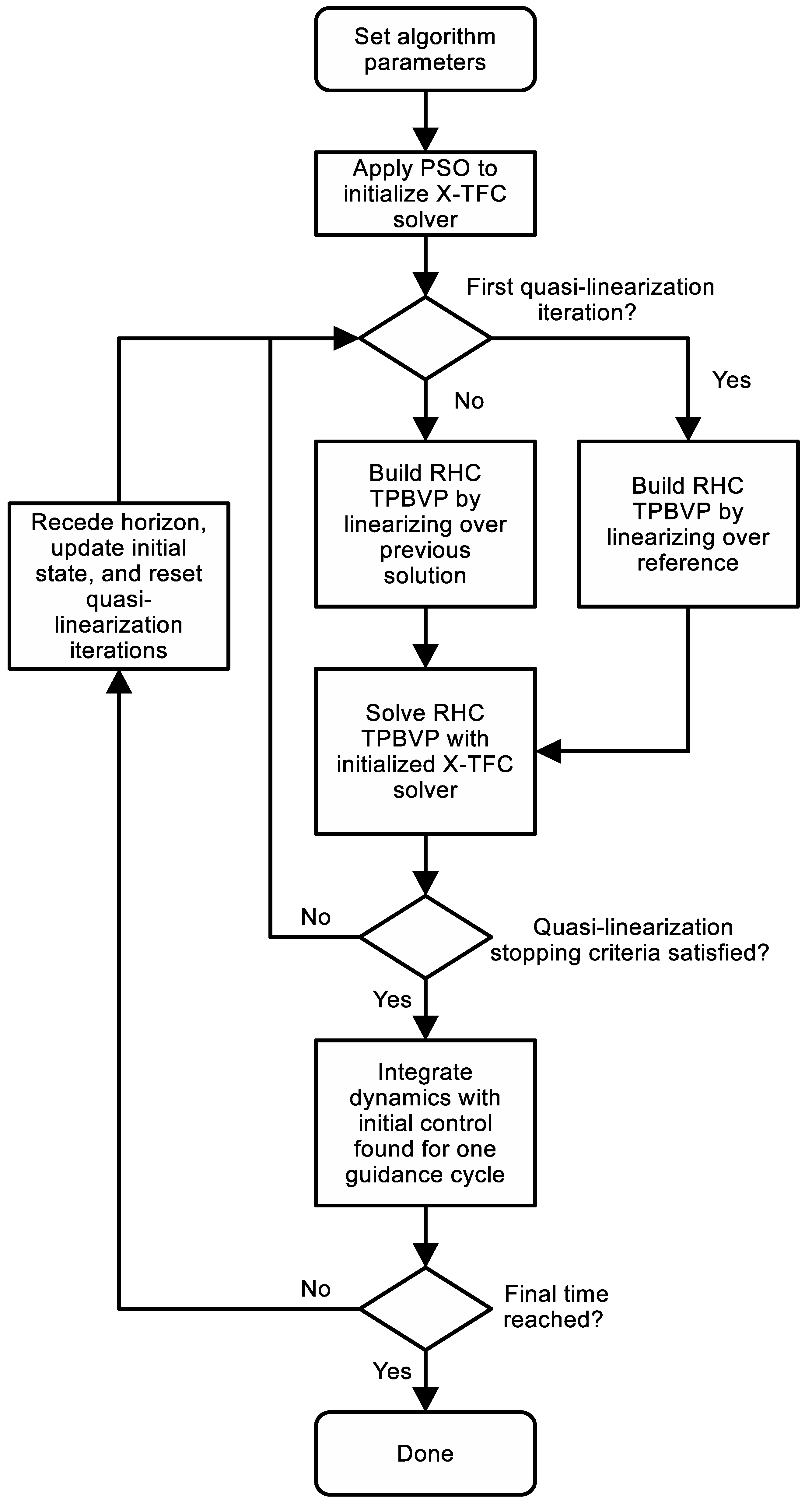
Figure A1. X-TFC-RHC algorithmic flowchart.
Mathematics 13 03717 g0a1

References

  1. Kwon, W.H.; Han, S.H. Receding Horizon Control: Model Predictive Control for State Models; Springer: Berlin/Heidelberg, Germany, 2006. [Google Scholar]
  2. Yan, H.; Fahroo, F.; Ross, I.M. Real-Time Computation of Neighboring Optimal Control Laws. In Proceedings of the AIAA Guidance, Navigation, and Control Conference and Exhibit, Monterey, CA, USA, 5–8 August 2002; p. 4657. [Google Scholar] [CrossRef]
  3. Williams, P. Application of Pseudospectral Methods for Receding Horizon Control. J. Guid. Control Dyn. 2004, 27, 310–314. [Google Scholar] [CrossRef]
  4. Yang, L.; Zhou, H.; Chen, W. Application of Linear Gauss Pseudospectral method in Model Predictive Control. Acta Astronaut. 2014, 96, 175–187. [Google Scholar] [CrossRef]
  5. Liao, Y.; Li, H.; Bao, W. Indirect Radau Pseudospectral Method for the Receding Horizon Control Problem. Chin. J. Aeronaut. 2016, 29, 215–227. [Google Scholar] [CrossRef]
  6. Gu, D.; Hu, H. Receding Horizon Tracking Control of Wheeled Mobile Robots. IEEE Trans. Control Syst. Technol. 2006, 14, 743–749. [Google Scholar] [CrossRef]
  7. Park, Y.; Shamma, J.S.; Harmon, T.C. A Receding Horizon Control Algorithm for Adaptive Management of Soil Moisture and Chemical Levels During Irrigation. Environ. Model. Softw. 2009, 24, 1112–1121. [Google Scholar] [CrossRef]
  8. Zavala, V.M.; Biegler, L.T. Optimization-Based Strategies for the Operation of Low-Density Polyethylene Tubular Reactors: Nonlinear Model Predictive Control. Comput. Chem. Eng. 2009, 33, 1735–1746. [Google Scholar] [CrossRef]
  9. Mayne, D.Q.; Rawlings, J.B.; Rao, C.V.; Scokaert, P.O. Constrained Model Predictive Control: Stability and Optimality. Automatica 2000, 36, 789–814. [Google Scholar] [CrossRef]
  10. Fontes, F.A. A General Framework to Design Stabilizing Nonlinear Model Predictive Controllers. Syst. Control Lett. 2001, 42, 127–143. [Google Scholar] [CrossRef]
  11. Tian, B.; Zong, Q. Optimal Guidance for Reentry Vehicles Based on Indirect Legendre Pseudospectral Method. Acta Astronaut. 2011, 68, 1176–1184. [Google Scholar] [CrossRef]
  12. Lu, P. Regulation about Time-Varying Trajectories: Precision Entry Guidance Illustrated. J. Guid. Control Dyn. 1999, 22, 784–790. [Google Scholar] [CrossRef]
  13. Bryson, A.E.; Ho, Y.C. Applied Optimal Control: Optimization, Estimation, and Control, 1st ed.; Taylor & Francis Group, LLC: New York, NY, USA, 1975. [Google Scholar]
  14. Yan, H.; Fahroo, F.; Ross, I.M. Optimal Feedback Control Laws by Legendre Pseudospectral Approximations. In Proceedings of the 2001 American Control Conference, (Cat. No. 01CH37148), Arlington, VA, USA, 25–27 June 2001; IEEE: New York, NY, USA, 2001; Volume 3, pp. 2388–2393. [Google Scholar] [CrossRef]
  15. Smith, H.A.; Chase, J.G.; Wu, W.H. Efficient Integration of the Time Varying Closed-Loop Optimal Control Problem. J. Intell. Mater. Syst. Struct. 1995, 6, 529–536. [Google Scholar] [CrossRef]
  16. Lu, P. Approximate Nonlinear Receding-Horizon Control Laws in Closed Form. Int. J. Control 1998, 71, 19–34. [Google Scholar] [CrossRef]
  17. Lu, P. Closed-Form Control Laws for Linear Time-Varying Systems. IEEE Trans. Autom. Control 2000, 45, 537–542. [Google Scholar] [CrossRef]
  18. Michalska, H.; Mayne, D.Q. Robust Receding Horizon Control of Constrained Nonlinear Systems. IEEE Trans. Autom. Control 1993, 38, 1623–1633. [Google Scholar] [CrossRef]
  19. Malanowski, K.D. Convergence of the Lagrange-Newton Method for Optimal Control Problems. Int. J. Appl. Math. Comput. Sci. 2004, 14, 531–540. [Google Scholar]
  20. Lee, E.S. Quasilinearization and Invariant Imbedding: With Applications to Chemical Engineering and Adaptive Control; Academic Press: Cambridge, MA, USA, 1968; Chapter 2; pp. 9–39. [Google Scholar]
  21. Jaddu, H. Direct Solution of Nonlinear Optimal Control Problems Using Quasilinearization and Chebyshev Polynomials. J. Frankl. Inst. 2002, 339, 479–498. [Google Scholar] [CrossRef]
  22. Xu, X.; Agrawal, S. Finite-Time Optimal Control of Polynomial Systems Using Successive Suboptimal Approximations. J. Optim. Theory Appl. 2000, 105, 477–489. [Google Scholar] [CrossRef]
  23. Peng, H.; Gao, Q.; Wu, Z.; Zhong, W. Efficient Sparse Approach for Solving Receding-Horizon Control Problems. J. Guid. Control Dyn. 2013, 36, 1864–1872. [Google Scholar] [CrossRef]
  24. Chen, Q.; Wang, X.; Yang, J. Optimal Path-Following Guidance with Generalized Weighting Functions Based on Indirect Gauss Pseudospectral Method. Math. Probl. Eng. 2018, 2018, 3104397. [Google Scholar] [CrossRef]
  25. Schiassi, E.; Furfaro, R.; Leake, C.; De Florio, M.; Johnston, H.; Mortari, D. Extreme Theory of Functional Connections: A fast Physics-Informed Neural Network Method for Solving Ordinary and Partial Differential Equations. Neurocomputing 2021, 457, 334–356. [Google Scholar] [CrossRef]
  26. Leake, C.; Johnston, H.; Daniele, M. The Theory of Functional Connections: A Functional Interpolation Framework with Applications; Lulu: Morrisville, NC, USA, 2022. [Google Scholar]
  27. Mortari, D. The Theory of Connections: Connecting Points. Mathematics 2017, 5, 57. [Google Scholar] [CrossRef]
  28. Mortari, D. Least-Squares Solution of Linear Differential Equations. Mathematics 2017, 5, 48. [Google Scholar] [CrossRef]
  29. De Florio, M.; Schiassi, E.; D’Ambrosio, A.; Mortari, D.; Furfaro, R. Theory of Functional Connections Applied to Linear ODEs Subject to Integral Constraints and Linear Ordinary Integro-Differential Equations. Math. Comput. Appl. 2021, 26, 65. [Google Scholar] [CrossRef]
  30. Mortari, D.; Johnston, H.; Smith, L. High Accuracy Least-Squares Solutions of Nonlinear Differential Equations. J. Comput. Appl. Math. 2019, 352, 293–307. [Google Scholar] [CrossRef] [PubMed]
  31. Schiassi, E.; D’Ambrosio, A.; Drozd, K.; Curti, F.; Furfaro, R. Physics-Informed Neural Networks for Optimal Planar Orbit Transfers. J. Spacecr. Rocket 2022, 59, 834–849. [Google Scholar] [CrossRef]
  32. D’ambrosio, A.; Schiassi, E.; Curti, F.; Furfaro, R. Pontryagin Neural Networks with Functional Interpolation for Optimal Intercept Problems. Mathematics 2021, 9, 996. [Google Scholar] [CrossRef]
  33. Kennedy, J.; Eberhart, R. Particle Swarm Optimization. In Proceedings of the ICNN’95-International Conference on Neural Networks, Perth, WA, Australia, 27 November–1 December 1995; IEEE: New York, NY, USA, 1995; Volume 4, pp. 1942–1948. [Google Scholar] [CrossRef]
  34. Johnston, H.; Schiassi, E.; Furfaro, R.; Mortari, D. Fuel-Efficient Powered Descent Guidance on Large Planetary Bodies via Theory of Functional Connections. J. Astronaut. Sci. 2020, 67, 1521–1552. [Google Scholar] [CrossRef]
  35. Drozd, K.; Furfaro, R.; Schiassi, E.; Johnston, H.; Mortari, D. Energy-Optimal Trajectory Problems in Relative Motion Solved via Theory of Functional Connections. Acta Astronaut. 2021, 182, 361–382. [Google Scholar] [CrossRef]
  36. Li, S.; Yan, Y.; Zhang, K.; Li, X. Fuel-Optimal Ascent Trajectory Problem for Launch Vehicle via Theory of Functional Connections. Int. J. Aerosp. Eng. 2021, 2021, 2734230. [Google Scholar] [CrossRef]
  37. Furfaro, R.; Mortari, D. Least-Squares Solution of a Class of Optimal Space Guidance Problems via Theory of Connections. Acta Astronaut. 2020, 168, 92–103. [Google Scholar] [CrossRef]
  38. de Almeida Junior, A.K.; Johnston, H.; Leake, C.; Mortari, D. Fast 2-impulse Non-Keplerian Orbit Transfer Using the Theory of Functional Connections. Eur. Phys. J. Plus 2021, 136, 1–21. [Google Scholar] [CrossRef]
  39. D’Ambrosio, A.; Schiassi, E.; Johnston, H.; Curti, F.; Mortari, D.; Furfaro, R. Time-Energy Optimal Landing on Planetary Bodies via Theory of Functional Connections. Adv. Space Res. 2022, 69, 4198–4220. [Google Scholar] [CrossRef]
  40. Antonelo, E.A.; Camponogara, E.; Seman, L.O.; Jordanou, J.P.; de Souza, E.R.; Hübner, J.F. Physics-Informed Neural Nets for Control of Dynamical Systems. Neurocomputing 2024, 579, 127419. [Google Scholar] [CrossRef]
  41. Li, Y.; Liu, L. Physics-Informed Neural Network-Based Nonlinear Model Predictive Control for Automated Guided Vehicle Trajectory Tracking. World Electr. Veh. J. 2024, 15, 460. [Google Scholar] [CrossRef]
  42. Johnston, H.; Leake, C.; Efendiev, Y.; Mortari, D. Selected Applications of the Theory of Connections: A Technique for Analytical Constraint Embedding. Mathematics 2019, 7, 537. [Google Scholar] [CrossRef]
  43. Buhmann, M.D. Radial Basis Functions: Theory and Implementations; Cambridge University Press: Cambridge, UK, 2003; Volume 12, Chapter 2. [Google Scholar]
  44. Huang, G.B.; Siew, C.K. Extreme Learning Machine: RBF Network Case. In Proceedings of the ICARCV 2004 8th Control, Automation, Robotics and Vision Conference, Kunming, China, 6–9 December 2004; IEEE: New York, NY, USA, 2004; Volume 2, pp. 1029–1036. [Google Scholar] [CrossRef]
  45. Fornberg, B.; Zuev, J. The Runge Phenomenon and Spatially Variable Shape Parameters in RBF Interpolation. Comput. Math. Appl. 2007, 54, 379–398. [Google Scholar] [CrossRef]
  46. Sing, J.; Basu, D.; Nasipuri, M.; Kundu, M. Improved K-means Algorithm in the Design of RBF Neural Networks. In Proceedings of the TENCON 2003, Conference on Convergent Technologies for Asia-Pacific Region, Bangalore, India, 15–17 October 2003; IEEE: New York, NY, USA, 2003; Volume 2, pp. 841–845. [Google Scholar] [CrossRef]
  47. Lim, E.A.; Zainuddin, Z. An Improved Fast Training Algorithm for RBF Networks Using Symmetry-Based Fuzzy C-means Clustering. MATEMATIKA Malays. J. Ind. Appl. Math. 2008, 24, 141–148. [Google Scholar] [CrossRef]
  48. He, J.; Liu, H. The Application of Dynamic K-means Clustering Algorithm in the Center Selection of RBF Neural Networks. In Proceedings of the 2009 Third International Conference on Genetic and Evolutionary Computing, Guilin, China, 14–17 October 2009; IEEE: New York, NY, USA, 2009; pp. 488–491. [Google Scholar] [CrossRef]
  49. Sarimveis, H.; Alexandridis, A.; Mazarakis, S.; Bafas, G. A New Algorithm for Developing Dynamic Radial Basis Function Neural Network Models Based on Genetic Algorithms. Comput. Chem. Eng. 2004, 28, 209–217. [Google Scholar] [CrossRef]
  50. Yuan, J.L.; Li, X.Y.; Zhong, L. Optimized Grey RBF Prediction Model Based on Genetic Algorithm. In Proceedings of the 2008 International Conference on Computer Science and Software Engineering, Wuhan, China, 12–14 December 2008; IEEE: New York, NY, USA, 2008; Volume 1, pp. 74–77. [Google Scholar] [CrossRef]
  51. Aljarah, I.; Faris, H.; Mirjalili, S.; Al-Madi, N. Training Radial Basis Function Networks Using Biogeography-Based Optimizer. Neural Comput. Appl. 2018, 29, 529–553. [Google Scholar] [CrossRef]
  52. Foqaha, M.; Awad, M. Hybrid Approach to Optimize the Centers of Radial Basis Function Neural Network Using Particle Swarm Optimization. J. Comput. 2017, 12, 396–407. [Google Scholar] [CrossRef]
  53. Sengupta, S.; Basak, S.; Peters, R.A. Particle Swarm Optimization: A Survey of Historical and Recent Developments with Hybridization Perspectives. Mach. Learn. Knowl. Extr. 2018, 1, 157–191. [Google Scholar] [CrossRef]
  54. Eberhart, R.C.; Shi, Y. Comparing Inertia Weights and Constriction Factors in Particle Swarm Optimization. In Proceedings of the 2000 Congress on Evolutionary Computation, CEC00 (Cat. No. 00TH8512), La Jolla, CA, USA, 16–19 July 2000; IEEE: New York, NY, USA, 2000; Volume 1, pp. 84–88. [Google Scholar] [CrossRef]
  55. Driscoll, T.A.; Heryudono, A.R. Adaptive Residual Subsampling Methods for Radial Basis Function Interpolation and Collocation Problems. Comput. Math. Appl. 2007, 53, 927–939. [Google Scholar] [CrossRef]
  56. Keerthi, S.S.; Gilbert, E.G. Optimal Infinite-Horizon Feedback Laws for a General Class of Constrained Discrete-Time Systems: Stability and Moving-Horizon Approximations. J. Optim. Theory Appl. 1988, 57, 265–293. [Google Scholar] [CrossRef]
  57. Mayne, D.Q.; Michalska, H. Receding Horizon Control of Nonlinear Systems. In Proceedings of the 27th IEEE Conference on Decision and Control, Austin, TX, USA, 7–9 December 1988; IEEE: New York, NY, USA, 1988; pp. 464–465. [Google Scholar] [CrossRef]
  58. Yang, T.; Polak, E. Moving Horizon Control of Nonlinear Systems with Input Saturation, Disturbances and Plant Uncertainty. Int. J. Control 1993, 58, 875–903. [Google Scholar] [CrossRef]
  59. De Nicolao, G.; Magni, L.; Scattolini, R. Stabilizing Receding-Horizon Control of Nonlinear Time-Varying Systems. IEEE Trans. Autom. Control 1998, 43, 1030–1036. [Google Scholar] [CrossRef]
  60. Jadbabaie, A.; Yu, J.; Hauser, J. Stabilizing Receding Horizon Control of Nonlinear Systems: A Control Lyapunov Function Approach. In Proceedings of the 1999 American Control Conference, San Diego, CA, USA, 2–4 June 1999; IEEE: New York, NY, USA, 1999; Volume 3, pp. 1535–1539. [Google Scholar] [CrossRef]
  61. Grüne, L.; Pannek, J. Nonlinear Model Predictive Control, 2nd ed.; Springer: Berlin/Heidelberg, Germany, 2017. [Google Scholar]
  62. Purwin, O.; D’Andrea, R. Performing Aggressive Maneuvers Using Iterative Learning Control. In Proceedings of the 2009 IEEE International Conference on Robotics and Automation, Kobe, Japan, 12–17 May 2009; IEEE: New York, NY, USA, 2009; pp. 1731–1736. [Google Scholar] [CrossRef]
  63. Lupashin, S.; Schöllig, A.; Sherback, M.; D’Andrea, R. A Simple Learning Strategy for High-Speed Quadrocopter Multi-Flips. In Proceedings of the 2010 IEEE International Conference on Robotics and Automation, Anchorage, AK, USA, 3–7 May 2010; IEEE: New York, NY, USA, 2010; pp. 1642–1648. [Google Scholar] [CrossRef]
  64. Ritz, R.; Hehn, M.; Lupashin, S.; D’Andrea, R. Quadrocopter Performance Benchmarking using Optimal Control. In Proceedings of the 2011 IEEE/RSJ International Conference on Intelligent Robots and Systems, San Francisco, CA, USA, 25–30 September 2011; IEEE: New York, NY, USA, 2011; pp. 5179–5186. [Google Scholar] [CrossRef]
  65. Tomić, T.; Maier, M.; Haddadin, S. Learning Quadrotor Maneuvers from Optimal Control and Generalizing in Real-Time. In Proceedings of the 2014 IEEE International Conference on Robotics and Automation (ICRA), Hong Kong, China, 31 May–5 June 2014; IEEE: New York, NY, USA, 2014; pp. 1747–1754. [Google Scholar] [CrossRef]
  66. Patterson, M.A.; Rao, A.V. GPOPS-II: A MATLAB Software for Solving Multiple-Phase Optimal Control Problems Using hp-Adaptive Gaussian Quadrature Collocation Methods and Sparse Nonlinear Programming. ACM Trans. Math. Softw. 2014, 41, 1–37. [Google Scholar] [CrossRef]
  67. Vinh, N.X.; Busemann, A.; Culp, R.D. Hypersonic and Planetary Entry Flight Mechanics; The University of Michigan Press: Ann Arbor, MI, USA, 1980; Chapter 2. [Google Scholar]
  68. Vaughan, D. A Negative Exponential Solution for the Matrix Riccati Equation. IEEE Trans. Autom. Control 1969, 14, 72–75. [Google Scholar] [CrossRef]
  69. Malkapure, H.G.; Chidambaram, M. Comparison of two Methods of Incorporating an Integral Action in Linear Quadratic Regulator. IFAC Proc. Vol. 2014, 47, 55–61. [Google Scholar] [CrossRef]
  70. He, L.; Zhang, R.; Li, H.; Bao, W. Physics Informed Neural Network Policy for Powered Descent Guidance. Aerosp. Sci. Technol. 2025, 167, 110656. [Google Scholar] [CrossRef]
  71. Williams, P. In-Plane Payload Capture with an Elastic Tether. J. Guid. Control Dyn. 2006, 29, 810–821. [Google Scholar] [CrossRef]
  72. Mai, T.; Mortari, D. Theory of Functional Connections Applied to Quadratic and Nonlinear Programming Under Equality Constraints. J. Comput. Appl. Math. 2021, 406, 113912. [Google Scholar] [CrossRef]
Figure 1. Plots of 5 GRBFs for different cases of center and shaping parameters selections: centers randomized between −1 and 1, and the shaping parameters randomized between 1 and 10 (a); centers placed on LGL collocation points and all shaping parameters set to 10 (b); centers placed on LGL collocation points and all shaping parameters set to 1 (c). Black circles are the LGL points. The x and y-axes are simply the domain and range of radial basis functions, respectively.
Mathematics 13 03717 g001
Figure 2. Low Earth orbit rendezvous position (a), velocity (b), and control (c) trajectories as N + 1 = L = 10 and T varies.
Mathematics 13 03717 g002
Figure 3. Planar quadrotor point-to-point tracking maneuver errors and cost difference when the quasi-linearized X-TFC-RHC controller has ε quasi = 1 × 10 6 and κ max between 1 and 10. The Δ refers to the difference of the tracking trajectory from the reference (ai).
Mathematics 13 03717 g003
Figure 4. A L 2 comparison as the method varied.
Mathematics 13 03717 g004
Figure 5. 500 Monte Carlo simulation of state (a), constraint (b), and control (c) trajectories where the initial state varied. Furthermore, the Monte Carlo L 2 results are also given (d).
Mathematics 13 03717 g005
Table 1. PSO hyperparameters.
ζ 1 ζ 2 ς ϵ min ϵ max ϵ min ϵ max a max N p
2.12.10.99605−0.10.1500100
Table 2. Computation time study.
N + 1 & LT (s) t cal_max ( 10 3 s) t cal_ave ( 10 3 s)
101009.4891.209
1210010.0601.513
1510010.5461.977
2010013.0442.829
5010025.71913.158
101259.8911.245
101509.5001.243
103009.7811.234
Table 3. Point-to-point maneuver tracking quasi-linearization errors between a highly accurate solution (where ε quasi = 10 10 ) and results where ε quasi varied.
ε quasi e ^ J e ^ x e ^ λ e ^ u
1 6.1 × 10 2 1.5 × 10 0 8.2 × 10 2 5.5 × 10 0
10 2 1.1 × 10 0 9.4 × 10 4 1.4 × 10 0 5.0 × 10 3
10 4 6.6 × 10 3 8.2 × 10 6 2.1 × 10 2 7.4 × 10 5
10 6 5.5 × 10 5 5.2 × 10 8 2.4 × 10 4 5.9 × 10 7
10 8 3.9 × 10 7 6.2 × 10 10 2.3 × 10 6 7.0 × 10 9
Table 4. Point-to-point maneuver tracking quasi-linearization errors between result of maximum iteration κ max and iteration κ max 1 .
κ e ¯ J e ¯ x e ¯ λ e ¯ u
1 3.2 × 10 3 2.6 × 10 2 1.2 × 10 5 2.6 × 10 2
5 1.2 × 10 1 3.3 × 10 1 2.2 × 10 2 6.4 × 10 1
10 2.6 × 10 2 3.0 × 10 4 2.7 × 10 1 4.7 × 10 4
15 3.1 × 10 5 3.4 × 10 7 3.5 × 10 4 5.4 × 10 7
20 5.6 × 10 8 1.1 × 10 9 7.6 × 10 7 1.3 × 10 9
Table 5. Computation time comparison between X-TFC-RHC and backward sweep method coupled with RHC.
Method N + 1 t cal_max ( 10 3 s) t cal_ave ( 10 3 s)
X-TFC106.5780.662
3111.6312.149
Backward Sweep10--
315.0022.276
Disclaimer/Publisher’s Note: The statements, opinions and data contained in all publications are solely those of the individual author(s) and contributor(s) and not of MDPI and/or the editor(s). MDPI and/or the editor(s) disclaim responsibility for any injury to people or property resulting from any ideas, methods, instructions or products referred to in the content.