Nonlocal Optimal Control in the Source—Numerical Approximation of the Compliance Functional Constrained by the p-Laplacian Equation

Abstract

The goal of this manuscript is the study of an optimal control problem. It consists on the minimization of the compliance functional when the state equation is the nonlocal p-laplacian and the control is the source of this equation. For this problem, a minimum principle, an uniqueness result of optimal control, and a numerical scheme able to approximate the only optimal control, have been derived. The obtained results are an extension of those found in the Cea and Malanowski’s paper, and the arguments employed to face the nonlinear and nonlocal case have been achieved by Muñoz. Some numerical examples are given.

1. Introduction

It is wellknown that the inherent properties of an optimization problem are almost always relevant for the design of a numerical algorithm. The finding of these features is helpful because they can help in the construction of new approximation methods for solutions. With this aim, we propose an extension of the results derived in [1]. Our purpose is to present a general minimum principle, an optimal control uniqueness result, and the application to develop a numerical scheme to approximate the solution. By following [2], we pose the problem within a nonlocal context, we establish the link between the nonlocal and local formulations, and we generalize the linear case by carrying out the study when the state equation is of nonlocal p-laplacian type with $p>1.$

In condensed form, the problem we shall study can be stated as follows: we consider the set of controls

$$\mathcal{F}=\left\{f\in L^{p^{\prime }}\left(\mathrm{\Omega }\right):{\int }_{\mathrm{\Omega }}f\left(x\right)\mathrm{d}x=C_1 \mathrm{and} {\int }_{\mathrm{\Omega }}{\left|f\left(x\right)\right|}^{p^{\prime }}\mathrm{d}x\le C_2\right\}$$

(1)

where $p>1,$$p^{\prime }={\displaystyle \frac{p}{p-1}}$, $C_1$ and $C_2>0$ are given constants, and $\mathrm{\Omega }$ is a smooth domain in ${\mathbb{R}}^N.$ The goal is to solve

$$\underset{f\in \mathcal{F}}{min}L\left(f\right)\doteq {\int }_{\mathrm{\Omega }}f\left(x\right)u\left(x\right)\mathrm{d}x,$$

(2)

that is, the minimization of the compliance functional L. The constraint $f\in \mathcal{F}$ means that the pair $\left(f,u\right)$ must satisfy the state equation

$$B_h\left(u,·\right)=f$$

(3)

As we have commented, the nonlocal differential operator $B_h\left(·,·\right)$ will be of p-laplacian type, with $p>1$, but formulated in a nonlocal frame.

It is well-known that $B_h\left(·,·\right)$ is an operator frequently employed to reproduce meaningful phenomena in Diffusion Theory, Conductivity Theory, and Materials Design [3,4,5,6]. In the nonlocal framework, the operator $B_h$ does not use gradients. In contrast, it accounts for the inter-relationship of the u-values evaluated at different points within an environment whose dimensions depend on the horizon parameter $\delta$. This parameter is the degree of exchange or nonlocality (see (10) for a precise formulation of (3)). For an understandable and detailed study of this kind of formulation, the reader can consult the book [7].

The optimization problem stated above has been quite frequently analyzed in the literature for the local case (see for instance [3,6,8,9,10]). Even though there is a large number of outstanding articles dealing with different nonlocal p-laplacian equations (see [7,11,12,13,14]), the nonlocal optimal control problem has not been studied so extensively. In either case, the present work deals with an elliptic optimal control problem where the control is at the right-hand side of the state equation, f, which we shall call the source. In (3), the coefficient h is the conductivity (or diffusion) of the material, which, throughout the manuscript, will be considered fixed. Another particular feature is the form of the cost functional L defined in (2). It has the peculiarity that can be expressed as the product of the electrical potential (or temperature) times the source applied to the system. Besides, it is often used to compute the energy dissipated inside $\mathrm{\Omega }$. Note that it can be directly written by using the form of the p-laplacian operator we have on the left-hand of the state equation, that is, $L\left(f\right)=B_h\left(u,u\right)$. This fact allows us to analyze the problem as a max-min problem (see [1,8,15]).

We recall that for meaningful problems we have approximation results according to which the local optimal control problem can be approximated by a sequence of nonlocal problems when the horizon tends to zero [16,17,18,19,20,21,22,23,24,25]. In [2] this is performed for general objective functionals, with the source playing the role of control and under non-homogeneous Dirichlet boundary conditions.

1.1. Hypotheses

We first introduce the hypotheses and pose the specific problems we want to solve. The framework in which we work includes a set $\mathrm{\Omega }\subset {\mathbb{R}}^N,$ which is assumed to be a smooth domain. We extend $\mathrm{\Omega }$ with a horizon $\delta >0$ ($\delta$ is a positive number) obtaining the domain ${\mathrm{\Omega }}_{\delta }=\mathrm{\Omega }{\cup }_{p\in \partial \mathrm{\Omega }}B\left(p,\delta \right)$. $B\left(x,r\right)$ is the notation of an open ball centered at $x\in {\mathbb{R}}^N$ and radius $r>0$.

About the source f, the right term of the elliptic equation, we assume $f\in L^{p^{\prime }}\left(\mathrm{\Omega }\right)$ where $p^{\prime }={\displaystyle \frac{p}{p-1}}$ and $p>1.$ Concerning the sequence of kernels ${\left(k_{\delta }\right)}_{\delta >0}$ involved in the description of our nonlocal model, we will assume that it is a sequence of nonnegative radial functions such that for any $\delta ,$

$$supp{k}_{\delta }\subset B\left(0,\delta \right)$$

(4)

and

$${\displaystyle \frac{1}{C_N}}{\int }_{B\left(0,\delta \right)}{k}_{\delta }\left(\left|z\right|\right)\mathrm{d}z=1$$

where $C_N={\displaystyle \frac{1}{meas\left(S^{N-1}\right)}}{\int }_{S^{N-1}}{\left|\omega ·e\right|}^{p}d{\sigma }^{N-1}\left(\omega \right),$${\sigma }^{N-1}$ stands for the $N-1$ dimensional Hausdorff measure on the unit sphere $S^{N-1}$ and e is any unitary vector in ${\mathbb{R}}^N.$ In addition, the kernels satisfy the uniform estimation

$$k_{\delta }\left(\left|z\right|\right)\ge {\displaystyle \frac{c_0}{{\left|z\right|}^{N+\left(s-1\right)p}}}$$

(5)

for $z\in supp{k}_{\delta },$ where $c_0>0$ and $s\in \left(0,1\right)$ are given constants.

The space in which we shall work is

$$X=\left\{u\in L^p\left({\mathrm{\Omega }}_{\delta }\right):B\left(u,u\right)<\infty \right\}$$

(6)

where $B:X\times X\to \mathbb{R}$ is the operator defined by the formula

$$B\left(u,v\right)={\int }_{{\mathrm{\Omega }}_{\delta }}{\int }_{{\mathrm{\Omega }}_{\delta }}{k}_{\delta }\left(\left|x^{\prime }-x\right|\right){\displaystyle \frac{{\left|u\left(x^{\prime }\right)-u\left(x\right)\right|}^{p-2}\left(u\left(x^{\prime }\right)-u\left(x\right)\right)}{{\left|x^{\prime }-x\right|}^p}}\left(v\left(x^{\prime }\right)-v\left(x\right)\right)\mathrm{d}{x}^{\prime }\mathrm{d}x.$$

(7)

We define also the constrained energy space as

$$X_0=\left\{u\in X:u=0 \mathrm{in} {\mathrm{\Omega }}_{\delta }\setminus \mathrm{\Omega }\right\}$$

It is wellknown that for any given $\delta >0$ the space $X=X\left(\delta \right)$ is a Banach space with the norm

$${∥u∥}_X={∥u∥}_{L^p\left({\mathrm{\Omega }}_{\delta }\right)}+{\left(B\left(u,u\right)\right)}^{1/p}.$$

The dual of X will be denoted by $X^{\prime }$ and can be endowed with the norm defined by

$${∥g∥}_{X^{\prime }}=sup\left\{{⟨g,w⟩}_{X^{\prime }\times X}:w\in X, {∥w∥}_X=1\right\}.$$

Analogous definitions apply to the space $X_0=X_0\left(\delta \right).$

There is another functional space that we will use in the formulation of the problem, the space of diffusion coefficients

$$\mathcal{H}\doteq \left\{h:{\mathrm{\Omega }}_{\delta }\to \mathbb{R}\mid h\left(x\right)\in [h_{min},h_{max}] \mathrm{a}.\mathrm{e}. x\in \mathrm{\Omega }, h=0 \mathrm{in} {\mathrm{\Omega }}_{\delta }-\mathrm{\Omega }\right\},$$

where $h_{min}$ and $h_{max}$ are positive constants such that $0<h_{min}<h_{max}.$

1.2. Formulation of the Problems

1.2.1. Nonlocal Optimal Control

The nonlocal optimal control problem in the source, denoted by $\left({\mathcal{P}}^{\delta }\right),$ is as follows: for each $\delta >0$ fixed, we look for $g\in L^{p^{\prime }}\left(\mathrm{\Omega }\right)$ such that minimizes the functional

$$I_{\delta }\left(g,u_g\right)={\int }_{\mathrm{\Omega }}F\left(x,u_g\left(x\right),g\left(x\right)\right)\mathrm{d}x,$$

(8)

where $u_g\in X$ solves the nonlocal boundary problem $\left(P^{\delta }\right)$

$$\left\{\begin{array}{c}\hfill {\displaystyle B_h\left(u_g,w\right)={\int }_{\mathrm{\Omega }}g\left(x\right)w\left(x\right)\mathrm{d}x, \mathrm{for} \mathrm{any} w\in X_0,}\\ {\displaystyle u_g=u_0 \mathrm{in} {\mathrm{\Omega }}_{\delta }\setminus \mathrm{\Omega },}\hfill \end{array} \right.$$

(9)

where

$$B_h\left(u,w\right)={\int }_{{\mathrm{\Omega }}_{\delta }}{\int }_{{\mathrm{\Omega }}_{\delta }}H\left(x^{\prime },x\right)k_{\delta }\left(\left|x^{\prime }-x\right|\right){\displaystyle \frac{{\left|u\left(x^{\prime }\right)-u\left(x\right)\right|}^{p-2}\left(u\left(x^{\prime }\right)-u\left(x\right)\right)}{{\left|x^{\prime }-x\right|}^p}}\left(v\left(x^{\prime }\right)-v\left(x\right)\right)\mathrm{d}{x}^{\prime }\mathrm{d}x$$

(10)

$H\left(x^{\prime },x\right)\doteq {\displaystyle \frac{h\left(x^{\prime }\right)+h\left(x\right)}{2}}$ and $u_0$ is a given function. The nonlocal boundary condition, $u=u_0$ in ${\mathrm{\Omega }}_{\delta }\setminus \mathrm{\Omega },$ must be interpreted in the sense of traces. Indeed, in order to make sense it is necessary that $u_0$ belongs to the space ${\tilde{X}}_0=\left\{{\left.w\right|}_{{\mathrm{\Omega }}_{\delta }\setminus \mathrm{\Omega }}:w\in X\right\}$. This space is well defined independently of the parameter $s\in \left(0,1\right)$ we choose in (5). It is easy to check that a norm for this space is the one defined as

$${∥v∥}_{{\tilde{X}}_0}=inf\left\{{∥w∥}_{L^p\left({\mathrm{\Omega }}_{\delta }\right)}+{\left(B\left(w,w\right)\right)}^{1/p}:w\in X \mathrm{such} \mathrm{that} {\left.w\right|}_{{\mathrm{\Omega }}_{\delta }\setminus \mathrm{\Omega }}=v\right\}.$$

The integrand F is under the format

$$F\left(x,u\left(x\right),g\left(x\right)\right)=G\left(x,u\left(x\right)\right)+\beta {\left|g\left(x\right)\right|}^{p^{\prime }}$$

(11)

where $\beta$ is a given positive constant, $h_0\in \mathcal{H}$ is also given, and $G:\mathbb{R}\times \mathbb{R}\to \mathbb{R}$ is a measurable positive function such that $G(x,·)$ is uniformly Lipschitz continuous (for any $x\in \mathrm{\Omega }$ and any $\left(u,v\right)\in {\mathbb{R}}^2$ there exists a positive constant L such that $\left|G\left(x,u\right)-G\left(x,v\right)\right|\le L\left|u-v\right|).$

We formulate the nonlocal optimal control problem as

$$\underset{\left(g,u\right)\in {\mathcal{A}}^{\delta }}{min}{I}_{\delta }\left(g,u_g\right)$$

(12)

where

$${\mathcal{A}}^{\delta }\doteq \left\{\left(f,v\right)\in L^{p^{\prime }}\left(\mathrm{\Omega }\right)\times \left(u_0+X_0\right):v \mathrm{solves} \left(9\right) \mathrm{with} g=f\right\}.$$

and

$$u_0+X_0\doteq \left\{v\in X:v=u_0+w \mathrm{where} w\in X_0\right\}.$$

1.2.2. Local Optimal Control

The local counterpart of (12), denoted by $\left({\mathcal{P}}^{loc}\right),$ is an optimal control problem whose goal is to find $g\in L^{p^{\prime }}\left(\mathrm{\Omega }\right)$ such that minimizes the functional

$$I\left(g,u_g\right)={\int }_{\mathrm{\Omega }}\left(G\left(x,u_g\left(x\right)\right)+\beta {\left|g\left(x\right)\right|}^{p^{\prime }}\right)\mathrm{d}x,$$

(13)

where $u_g\in W^{1,p}\left(\mathrm{\Omega }\right)$ is the solution of the local boundary problem $\left(P^{loc}\right)$

$$\left\{\begin{array}{c}\hfill {\displaystyle b_h\left(u_g,w\right)={\int }_{\mathrm{\Omega }}g\left(x\right)w\left(x\right)\mathrm{d}x, \mathrm{for} \mathrm{any} w\in W_0^{1,p}\left(\mathrm{\Omega }\right)}\\ {\displaystyle u_g=u_0 \mathrm{in} \partial \mathrm{\Omega },}\hfill \end{array} \right.$$

(14)

$b\left(·,·\right)$ is the operator defined in $W^{1,p}\left(\mathrm{\Omega }\right)\times W^{1,p}\left(\mathrm{\Omega }\right)$ by means of

$$b_h\left(u,v\right)\doteq {\int }_{\mathrm{\Omega }}h\left(x\right){\left|\nabla u\left(x\right)\right|}^{p-2}\nabla u\left(x\right)\nabla v\left(x\right)\mathrm{d}x,$$

$h_0\in \mathcal{H}$ and $u_0$ is a given function from the trace fractional Sobolev space $W^{1-1/p,p}\left(\partial \mathrm{\Omega }\right)$.

The statement of the local optimal control problem is

$$\underset{\left(g,u\right)\in {\mathcal{A}}^{loc}}{min}I\left(g,u_g\right)$$

(15)

where

$${\mathcal{A}}^{loc}\doteq \left\{\left(f,v\right)\in L^{p^{\prime }}\left(\mathrm{\Omega }\right)\times \left(u_0+W_0^{1,p}\left(\mathrm{\Omega }\right)\right):v \mathrm{solves} \left(14\right) \mathrm{with} g=f\right\}.$$

with

$$u_0+W_0^{1,p}\left(\mathrm{\Omega }\right)\doteq \left\{v\in W^{1,p}\left(\mathrm{\Omega }\right):v=u_0+w \mathrm{where} w\in W_0^{1,p}\left(\mathrm{\Omega }\right)\right\}.$$

The analysis of this type of problem has been extensively studied in previous works [2,22,26,27,28,29]. The paper [21] starts the study on the optimization when the control is the source and the state equations are of nonlocal elliptic type. After, a series of articles containing different types of controls has appeared in recent years. Refs. [22,30,31] are meaningful works dealing with nonlocal control problems. About the asymptotic analysis, refs. [7,18,20,21,23,24,25,32,33,34,35] are papers where the reader can get a fairly detailed idea of this issue. Much more should be commented about the influence that this type of problems has received from an outstanding list of seminal papers [7,11,19,34,36,37,38].

In what concerns the numerical analysis of nonlocal problems, refs. [39,40,41,42,43,44] are references of interest. In [45] an extensive discussion about different numerical methods for the nonlocal fractional diffusion model can be found. They discuss several methods, finite element, finite differences or spectral methods. It shows part of the most recent mathematical and computational developments applied to the analysis of nonlocal peridynamic models. About the approximation of nonlocal optimal controls, we refer [21] as a pioneering work in this area. See also [22,46,47,48,49,50].

1.3. Results and Organization

The novelty of this work is the derivation of a minimum principle, a uniqueness result and a convergent descent method in a nonlocal control problem where the state equation is the p-laplacian with $p>1$. The organization of the article to show these contributions is as follows: in the first part of Section 2, some specific preliminary results concerning elementary inequalities and compactness are explained. Section 2.2 and Section 2.3 contain the main issues concerning the state equation and the processes of G-convergence. For the details, see [2] and references therein. Section 3 is devoted to establishing the minimum principle and the uniqueness of optimal control. These facts will make possible the numerical scheme from Section 4. The direction of descent, the size of the step and the convergence of the scheme are the aim of that section. Section 5 contains the numerical approximation for some concrete examples.

The summary of results of the present manuscript is:

1.

The derivation of a minimum principle as a tool to characterize optimal controls. See Theorems 6 and 8.

2.

Uniqueness of optimal control. See Corollary 1 and Theorem 7.

3.

Numerical algorithm based on the minimum principle. See Section 4.

4.

Convergence of the numerical procedure towards the unique optimal control (Theorem 10).

5.

Explicit numerical approximations both for the nonlocal and local problem (with $\delta$ small enough). Section 5 shows the result of some numerical simulations for the case $p=2.$

2. Preliminary Results, Well-Posedness of the State Equation and G-Convergence

2.1. Preliminaries

Here we review some technical tools that will be used.

1.

Compactness: the embedding

$$X_0\subset L^p\left(\mathrm{\Omega }\right)$$

is compact. In order to check that we first notice $X_0\subset W^{s,p}\left({\mathrm{\Omega }}_{\delta }\right),$ and since the elements of $X_0$ vanish in ${\mathrm{\Omega }}_{\delta }\setminus \mathrm{\Omega },$ then extension by zero outside ${\mathrm{\Omega }}_{\delta }$ gives rise to elements of $W^{s,p}\left({\mathbb{R}}^N\right)$ (see [37], Lemma 5.1). Then

$$X_0\subset W_0^{s,p}\left(\mathrm{\Omega }\right)=\left\{f\in W^{s,p}\left({\mathbb{R}}^N\right):f=0 \mathrm{in} {\mathbb{R}}^N\setminus \mathrm{\Omega }\right\}$$

2.

Nonlocal Poincaré inequality: we are in position to ensure the existence of a constant $c=c\left(N,s,p\right)$ such that for any $w\in X_0$

$$c{∥w∥}_{L^p\left({\mathrm{\Omega }}_{\delta }\right)}^p\le {\int }_{{\mathrm{\Omega }}_{\delta }}{\int }_{{\mathrm{\Omega }}_{\delta }}{\displaystyle \frac{{\left|w\left(x^{\prime }\right)-w\left(x\right)\right|}^p}{{\left|x^{\prime }-x\right|}^{N+sp}}}\mathrm{d}{x}^{\prime }\mathrm{d}x$$

(16)

(see [37], Th. 6.5). Under the hypotheses on the kernels (5), and using (16) we confirm there is a constant $C>0$ such that

$$C{∥w∥}_{L^p\left({\mathrm{\Omega }}_{\delta }\right)}^p\le B_h\left(w,w\right).$$

(17)

holds for any $w\in X_0.$

If we consider a sequence ${\left(w_j\right)}_j\in X_0$ and we assume there is $C>0$ such that $B_h\left(w_j,w_j\right)\le C$ for every $j,$ then by (17) ${\left(w_j\right)}_j$ is uniformly bounded in $L^p\left({\mathrm{\Omega }}_{\delta }\right)$ which, jointly with the above compactness result (see [37], Th. 7.1 ) allow us to ensure the existence of a subsequence from ${\left(w_j\right)}_j,$ still denoted by ${\left(w_j\right)}_j,$ such that $w_j\to w$ strongly in $L^p\left({\mathrm{\Omega }}_{\delta }\right),$ for some $w\in X_0.$ The same is true for any sequence ${\left(w_j\right)}_j\in u_0+X_0.$

3.

Let ${\left(g_{\delta },u_{\delta }\right)}_{\delta }$ be a sequence of admissible pairs verifying the uniform estimate

$$B_h\left(u_{\delta },u_{\delta }\right)\le C,$$

(here C is a positive constant). Then, from ${\left(u_{\delta }\right)}_{\delta }$ we can extract a subsequence, labelled also by $u_{\delta },$ such that $u_{\delta }\to u$ strongly in $L^p\left(\mathrm{\Omega }\right)$ and $u\in W^{1,p}\left(\mathrm{\Omega }\right)$ (see [51], Th. 1.2). Furthermore, the following inequality is fulfilled

$$\underset{\delta \to 0}{lim}{B}_h\left(u_{\delta },u_{\delta }\right)\ge {\int }_{\mathrm{\Omega }}h\left(x\right){\left|\nabla u\left(x\right)\right|}^{p}dx$$

(18)

(see [51,52,53]). Besides, it is also wellknown that if $u_{\delta }=u\in W^{1,p}\left(\mathrm{\Omega }\right),$ then the above limit is

$$\underset{\delta \to 0}{lim}{B}_h\left(u,u\right)={\int }_{\mathrm{\Omega }}h\left(x\right){\left|\nabla u\left(x\right)\right|}^{p}dx$$

(19)

(see [36], Cor. 1 and [17], Th. 8).

2.2. The State Equation

There is an essential result of characterization for the solution of the state equation. Let us assume $u_0\in {\tilde{X}}_0,$$\delta >0$ and g$\in L^{p^{\prime }}\left(\mathrm{\Omega }\right)$ are fixed.

Theorem 1

(Dirichlet Principle [2]).

1.

There exists a solution $u_g\in u_0+X_0$ to the minimization problem

$$\underset{w\in u_0+X_0}{min}\mathcal{J}\left(w\right)$$

(20)

where

$$\mathcal{J}\left(w\right)\doteq {\displaystyle \frac{1}{p}}{B}_h\left(w,w\right)-{\int }_{\mathrm{\Omega }}g\left(x\right)w\left(x\right)\mathrm{d}x.$$

2.

$u_g$ is a solution of the minimization principle (20) if, and only if, $u_g$ solves the problem (9).

3.

There exists a unique solution to the nonlocal boundary problem $\left(P^{\delta }\right)$ given in (9).

Remark 1.

We note the following technical result concerning the monotonicity of the nonlocal p-laplacian operator $B_h$: if $1<p<\infty ,$ then there exist two positive constants $C=C\left(p\right)$ and $c=c\left(p\right)$ such that for every $a,$ $b\in {\mathbb{R}}^{+}$

$$c{\left\{\left|a\right|+\left|b\right|\right\}}^{p-2}{\left|a-b\right|}^2\le \left({\left|a\right|}^{p-2}a-{\left|b\right|}^{p-2}b\right)\left(a-b\right)\le C{\left\{\left|a\right|+\left|b\right|\right\}}^{p-2}{\left|a-b\right|}^2.$$

(21)

(see [54], Prop.17.3 and Th. 17.1). In particular

$$c{\left|a-b\right|}^p\le \left({\left|a\right|}^{p-2}a-{\left|b\right|}^{p-2}b\right)\left(a-b\right)$$

(22)

where $c=arg{min}_{z\in {\mathbb{R}}^{+}}{\displaystyle \frac{1-z^{p-1}}{{\left(1+z\right)}^{p-2}\left(1-z\right)}}=\left(p-1\right)e^{-\left(p-2\right)\left(log2\right)}.$

2.3. G-Convergence for the State Equation

Let ${\left(g_j\right)}_j$ be a minimizing sequence of controls for the problem $\left({\mathcal{P}}^{\delta }\right)$ and let ${\left(u_j\right)}_j$ be the corresponding sequence of states. We shall assume that there is a constant $C>0$ such that for any ${\int }_{\mathrm{\Omega }}{\left|g_j\left(x\right)\right|}^{p^{\prime }}dx<C.$ Hence, Hölder and Young inequalities allow us to write

$$\left(1-{\displaystyle \frac{1}{p^{\prime }}}\right)B_h\left(u_j,u_j\right)\le C+D{\left(B_h\left(u_j,u_j\right)\right)}^{1/p}$$

for some positive constants C and $D.$ The above inequality implies $B_h\left(u_j,u_j\right)$ is uniformly bounded and ${∥u_j∥}_{L^p}$ too. If at this point we use point Part 2 from Section 2.1, we can state the strong convergence in $L^p$, at least for a subsequence of ${\left(u_j\right)}_j,$ to some function $u^{*}\in u_0+X_0.$ Let u be the state associated to $g.$ We pose the G-convergence, to check whether $u=u^{*}$ is true or not:

Theorem 2

(G-convergence [2]). Under the above circumstances we have:

1.

$$\begin{array}{c} \underset{j\to \infty }{lim}\underset{w\in u_0+X_0}{min}\left\{{\displaystyle \frac{1}{p}}{B}_h\left(w,w\right)-{\int }_{\mathrm{\Omega }}{g}_j\left(x\right)w\left(x\right)\mathrm{d}x\right\}\hfill \\ =\underset{w\in u_0+X_0}{min}\left\{{\displaystyle \frac{1}{p}}{B}_h\left(w,w\right)-{\int }_{\mathrm{\Omega }}g\left(x\right)w\left(x\right)\mathrm{d}x\right\}\hfill \end{array}$$

and $u=u^{*}.$

2.

$$\underset{j\to \infty }{lim}{B}_h\left(u_j,u_j\right)=B_h\left(u,u\right),$$

(23)

and

$$\underset{j\to \infty }{lim}{B}_h\left(u_j-u,u_j-u\right)=0.$$

(24)

Remark 2.

The convergence (23), together with the strong convergence of ${\left(u_j\right)}_j,$ is precisely equivalent to the strong convergence in X. We also realize that for any $h_0\in \mathcal{H}$

$$\underset{j\to \infty }{lim}{B}_{h_0}\left(u_j-u,u_j-u\right)=0$$

(25)

Remark 3.

The convergences of the states we have just described above, are still valid if we consider a sequence of sources ${\left(g_j\right)}_j$, uniformly bounded in the dual space $X_0^{\prime }.$

Theorem 3

(Well posedness [2]). For each $\delta >0$ there exists a solution $\left(g,u_{\delta }\right)$ to the control problem $\left({\mathcal{P}}^{\delta }\right)$ given in (12).

2.4. G-Convergence for the Nonlocal Optimal Control Problem

Assume the source g and $u_0\in W^{1-1/p,p}\left(\partial \mathrm{\Omega }\right)$ are fixed functions. If, for each $\delta ,$ we consider the corresponding sequence of states ${\left(u_{\delta }\right)}_{\delta }\subset u_0+W_0^{1,p}\left(\mathrm{\Omega }\right),$ then

$$B_h\left(u_{\delta },v\right)=\int g\left(x\right)v\left(x\right)\mathrm{d}x$$

for any $v\in X_0.$ As in the previous sections, we easily prove ${∥u_{\delta }∥}_{L^p\left(\mathrm{\Omega }\right)}$ and $B_h\left(u_{\delta },u_{\delta }\right)$ are sequences uniformly bounded in $\delta .$ Then, by using part 3 from Section 2.1, these estimations imply the existence of a function $u^{*}\in u_0+W_0^{1,p}\left(\mathrm{\Omega }\right)$ and a subsequence of $u_{\delta }$ (still denoted $u_{\delta })$, such that $u_{\delta }\to u^{*}$ strongly in $L^p\left(\mathrm{\Omega }\right)$. The question is to look for the state equation that should be satisfied by the pair $\left(g,u^{*}\right)$. The answer to this question is given in the following convergence result:

Theorem 4

([2]).

$$\begin{array}{c}{\displaystyle \underset{\delta \to 0}{lim}\underset{w\in u_0+X_0}{min}\left\{\frac{1}{p}{B}_h\left(w,w\right)-\int g\left(x\right)w\left(x\right)\mathrm{d}x\right\}}\hfill \\ {\displaystyle =\underset{w\in u_0+W_0^{1,p}\left(\mathrm{\Omega }\right)}{min}\left\{\frac{1}{p}{\int }_{\mathrm{\Omega }}h\left(x\right){\left|\nabla w\left(x\right)\right|}^p\mathrm{d}x-\int g\left(x\right)w\left(x\right)\mathrm{d}x\right\}}\hfill \end{array}$$

(26)

and $\left(g,u^{*}\right)\in {\mathcal{A}}^{loc}.$ Besides, the following convergence of energies holds:

$$\underset{\delta \to 0}{lim}{B}_h\left(u_{\delta },u_{\delta }\right)=b_h\left(u,u\right).$$

(27)

2.5. Approximation to the Optimal Source

We know that, for each $\delta ,$ there exists at least a solution $\left(g_{\delta },u_{\delta }\right)$ to the problem (12). Our purpose is to analyze asymptotically this sequence of solutions.

Theorem 5

([2]). Let $\left(g_{\delta },u_{\delta }\right)$ be the sequence of solutions to the control problem (12). Then there exists a pair $\left(g,u\right)\in L^{p^{\prime }}\left(\mathrm{\Omega }\right)\times \left(u_0+W_0^{1,p}\left(\mathrm{\Omega }\right)\right)$ and a subsequence of indexes δ for which the following conditions hold:

1.

$g_{\delta }\rightharpoonup g$ weakly in $L^{p^{\prime }}\left(\mathrm{\Omega }\right),$$u_{\delta }\to u$ strongly in $L^p\left(\mathrm{\Omega }\right)$ as $\delta \to 0.$

2.

$$\begin{array}{c}{\displaystyle \underset{\delta \to 0}{lim}\underset{w\in u_0+X_0}{min}\left\{\frac{1}{p}{B}_h\left(w,w\right)-\int g_{\delta }\left(x\right)w\left(x\right)\mathrm{d}x\right\}}\hfill \\ {\displaystyle =\underset{w\in u_0+W_0^{1,p}\left(\mathrm{\Omega }\right)}{min}\left\{\frac{1}{p}{b}_h\left(w,w\right)-\int g\left(x\right)w\left(x\right)\mathrm{d}x\right\}}\hfill \end{array}$$

(28)

and $\left(g,u\right)\in {\mathcal{A}}^{loc}.$

3.

$\left(g,u\right)$ is a solution to the local control problem (15).

$$\underset{\delta \to 0}{lim}{B}_h\left(u_{\delta },u_{\delta }\right)=b_h\left(u,u\right).$$

3. Approximation

Throughout the remainder of the paper, the cost functional will be the compliance: for a given $f,$ we consider its state $u_f$ and then, the aim is to solve

$$\underset{f\in }{min}{I}_{\delta }\left(f,u_f\right)={\int }_{\mathrm{\Omega }}f{u}_f\mathrm{d}x.$$

Thus, we have put $\beta =0$ and $G\left(x,u,g\right)=gu$ in (13) for the formulation of (15). We must remark that all the above results remain valid for this specific functional. A brief inspection shows Theorems 4 and 5 of article [2] still hold true if $\gamma =\beta =0$ and the cost is the compliance functional. Also, for the clarity of the exposition, without loss of generality, we shall assume $u_0=0$. Since $\delta$ is fixed we omit this index and we write the action of the functional on the pair $\left(f,u_f\right)\in {\mathcal{A}}^{\delta }$ as $L\left(f\right)={\int }_{\mathrm{\Omega }}f{u}_f.$ Consequently our problem is

$$\underset{\left(f,u_f\right)\in {\mathcal{A}}^{\delta }}{min}L\left(f\right)$$

(29)

where the set of admissible pairs is

$${\mathcal{A}}^{\delta }=\left\{\left(f,v\right)\in \mathcal{F}\times X_0:v \mathrm{solves} \left(9\right) \mathrm{with} g=f\right\}.$$

(30)

Remark 4.

The local counterpart of (29) and (30) is given by

$$\underset{\left(f,u_f\right)\in {\mathcal{A}}^{loc}}{min}L\left(f\right)$$

(31)

where

$${\mathcal{A}}^{loc}\doteq \left\{\left(f,v\right)\in \mathcal{F}\times W_0^{1,p}\left(\mathrm{\Omega }\right):v \mathit{solves} \left(14\right) \mathit{with} g=f\right\}.$$

(32)

Therefore, by invoking Theorem 4, if $\delta \to 0$ the solution of (29) and (30) converges to a solution of (31) and (32) (in fact, it will converge to the only solution of (31) and (32)).

Minimum Principle

Definition 1.

It is said that the admissible pair $\left(f,u_f\right)$ satisfies the minimum principle if

$$L\left(f\right)=\int f{u}_f=B_h\left(u_f,u_f\right)\le \int g{u}_f \mathit{for} \mathit{all} g\in \mathcal{F}.$$

Theorem 6.

If the pair $\left(f,u_f\right)$ is a solution of the problem (29) and (30) then it satisfies the minimum principle.

Proof. 

We consider the admissible source $f+\mathrm{\Delta }f=f+\rho \left(g-f\right)$ (where g $\in \mathcal{F}$). Then, the underlying state of $f+\mathrm{\Delta }f,$ $u_{f+\mathrm{\Delta }f},$ can be written as

$$u_{f+\mathrm{\Delta }f}=u_f+\mathrm{\Delta }{u}_f$$

Since at $\left(f,u_f\right)$ the minimum is attained,

$$B_h\left(u_f,u_f\right)=\int f{u}_f,$$

and

$$B_h\left(u_f+\mathrm{\Delta }{u}_f,u_f+\mathrm{\Delta }{u}_f\right)=\int \left(f+\mathrm{\Delta }f\right)\left(u_f+\mathrm{\Delta }{u}_f\right),$$

then

$$0\le B_h\left(u_f+\mathrm{\Delta }{u}_f,u_f+\mathrm{\Delta }{u}_f\right)-B_h\left(u_f,u_f\right)=\int f\mathrm{\Delta }{u}_f+\mathrm{\Delta }f{u}_f+\mathrm{\Delta }f\mathrm{\Delta }{u}_f.$$

(33)

Also, $\left(f,u_f\right)$ satisfies the state equation, which thanks to Theorem 1 implies

$${\displaystyle \frac{1}{p}}{B}_h\left(u_f,u_f\right)-\int f{u}_f\le {\displaystyle \frac{1}{p}}{B}_h\left(u_f+\mathrm{\Delta }{u}_f,u_f{u}_f+\mathrm{\Delta }{u}_f\right)-\int f\left(u_f+\mathrm{\Delta }{u}_f\right)$$

from where and by using (33) we have

$$\begin{array}{cc}\hfill B_h\left(u_f,u_f\right)& \le B_h\left(u_f+\mathrm{\Delta }{u}_f,u_f{u}_f+\mathrm{\Delta }{u}_f\right)\hfill \\ \hfill & -p\left[B_h\left(u_f+\mathrm{\Delta }{u}_f,u_f+\mathrm{\Delta }{u}_f\right)-B_h\left(u_f,u_f\right)-\int \mathrm{\Delta }f{u}_f-\mathrm{\Delta }f\mathrm{\Delta }{u}_f\right],\hfill \end{array}$$

that is

$$\left(p-1\right)\left[B_h\left(u_f+\mathrm{\Delta }{u}_f,u_f+\mathrm{\Delta }{u}_f\right)-B_h\left(u_f,u_f\right)\right]\le \int p\mathrm{\Delta }f{u}_f+p\mathrm{\Delta }f\mathrm{\Delta }{u}_f$$

Then, again by minimality ($B_h\left(u_f+\mathrm{\Delta }{u}_f,u_f+\mathrm{\Delta }{u}_f\right)-B_h\left(u_f,u_f\right)\ge 0)$ we deduce

$$\int \mathrm{\Delta }f\left[u_f+\mathrm{\Delta }{u}_f\right]\ge 0.$$

By dividing by $\rho$ we obtain

$$\int \left(g-f\right)u_f+\int \left(g-f\right)\mathrm{\Delta }{u}_f\ge 0$$

And by employing now the convergence of $\mathrm{\Delta }{u}_f$ if $\rho \to 0$ (Theorem 4) we arrive at

$$\int \left(g-f\right)u_f\ge 0,$$

which is what we were keen to try out. □

Theorem 7.

If $\left(f,u_f\right)$ is a solution of the problem (29) and (30) and $\left(g,u_g\right)$ is an admissible pair satisfying the minimum principle, then $u_f=u_g.$

Proof. 

The hypotheses and the previous result ensure

$$\int \left(G-f\right)u_f\ge 0$$

(34)

and

$$\int \left(G-g\right)u_g\ge 0$$

(35)

for any $G\in \mathcal{F}$. It is also true that the characterization of the admissible pairs (Theorem 1) and (34) provide

$$\begin{array}{cc}\hfill \underset{w}{min}\left\{{\displaystyle \frac{1}{p}}B\left(w,w\right)-\int fw\right\}& ={\displaystyle \frac{1}{p}}{B}_h\left(u_f,u_f\right)-\int f{u}_f\hfill \\ \hfill & \ge {\displaystyle \frac{1}{p}}{B}_h\left(u_f,u_f\right)-\int g{u}_f\hfill \\ \hfill & \ge {\displaystyle \frac{1}{p}}{B}_h\left(u_g,u_g\right)-\int g{u}_g\hfill \\ \hfill & =\underset{w}{min}\left\{{\displaystyle \frac{1}{p}}{B}_h\left(w,w\right)-\int gw\right\}.\hfill \end{array}$$

But again, the same reasoning with (35) gives

$$\underset{w}{min}\left\{{\displaystyle \frac{1}{p}}{B}_h\left(w,w\right)-\int gw\right\}\ge \underset{w}{min}\left\{{\displaystyle \frac{1}{p}}{B}_h\left(w,w\right)-\int fw\right\}$$

Then, both $u_f$ and $u_g$ are solutions of ${min}_w\left\{{\displaystyle \frac{1}{p}}{B}_h\left(w,w\right)-\int fw\right\}.$ The uniqueness of solution of this problem guarantees $u_f=u_g.$ □

Corollary 1.

If $\left(f,u_f\right)$ and $\left(g,u_g\right)$ are solutions of the problem (29) and (30), then

$$\underset{w}{min}\left\{{\displaystyle \frac{1}{p}}{B}_h\left(w,w\right)-\int fw\right\}=\underset{w}{min}\left\{{\displaystyle \frac{1}{p}}{B}_h\left(w,w\right)-\int gw\right\}$$

and $u_f=u_g.$ Moreover, $f=g.$

For the remainder of the proof, it suffices to notice that $B_h\left(u_f,\psi \right)=\int f\psi$ and $B_h\left(u_g,\psi \right)=\int g\psi ,$ for any $\psi \in X_0,$ and $u_f=u_g$. Indeed, these identities clearly imply $B_h\left(u_f,\psi \right)=B_h\left(u_g,\psi \right)$ for any $\psi \in X_0,$ which reads as $\int f\psi =\int g\psi ,$ for any $\psi \in X_0$ and whence we ensure $f=g.$

Theorem 8.

$\left(f,u_f\right)$ is an admissible pair satisfying the minimum principle if and only if it is the unique solution of (29) and (30).

Proof. 

If $\left(f,u_f\right)$ satisfies the minimum principle and $\left(g,w_g\right)$ is any other admissible pair, then

$$\begin{array}{cc}\hfill \left({\displaystyle \frac{1}{p}}-1\right)B_h\left(u_f,u_f\right)& ={\displaystyle \frac{1}{p}}{B}_h\left(u_f,u_f\right)-\int f{u}_f\hfill \\ \hfill & \ge {\displaystyle \frac{1}{p}}{B}_h\left(u_f,u_f\right)-\int g{u}_f\hfill \\ \hfill & \ge \underset{v}{inf}\left\{{\displaystyle \frac{1}{p}}{B}_h\left(v,v\right)-\int gv\right\}\hfill \\ \hfill & ={\displaystyle \frac{1}{p}}{B}_h\left(w_g,w_g\right)-\int g{w}_g\hfill \\ \hfill & =\left({\displaystyle \frac{1}{p}}-1\right)B_h\left(w_g,w_g\right)\hfill \end{array}$$

which amounts to say that $\left(f,u_f\right)$ is the optimal control. □

4. Algorithm

We assume the admissible pair $\left(f_r,u_r\right)$ at the step r is given. The cost corresponding to this pair is

$$L\left(f_r\right)=B_h\left(u_r,u_r\right)=\int f_r{u}_r$$

We look for $\left(f_{r+1},u_{r+1}\right)$ such that $f_{r+1}=f_r+\rho \left(g-f_r\right)=f_r+\mathrm{\Delta }{f}_r,$ where $g\in \mathcal{F}$ and $\rho \in \left(0,1\right).$ Thus, the task is to find the direction g and the size of the step $\rho .$ The underlying state of $f_{r+1}$ is denoted by $u_{r+1}=u_r+\mathrm{\Delta }{u}_r$ and the value of its cost is

$$L\left(f_{r+1}\right)=B_h\left(u_r+\mathrm{\Delta }{u}_r,u_r+\mathrm{\Delta }{u}_r\right)=\int \left(f_r+{\rho }_r\left(g-f_r\right)\right)\left(u_r+\mathrm{\Delta }{u}_r\right).$$

Then we consider the increment of the cost, which is defined as

$$E_r\doteq B_h\left(u_r,u_r\right)-B_h\left(u_r+\mathrm{\Delta }{u}_r,u_r+\mathrm{\Delta }{u}_r\right).$$

It is immediate to check

$$E_r=-\int f_r\mathrm{\Delta }{u}_r-\int \mathrm{\Delta }{f}_r\left(u_r+\mathrm{\Delta }{u}_r\right)$$

(36)

This section is devoted to choosing g and $\rho .$ We divide the study into three steps:

4.1. Direction

We look for the optimal $g.$ Since the pair $\left(f_r,u_r\right)$ is admissible we have

$${\displaystyle \frac{1}{p}}{B}_h\left(u_r,u_r\right)-\int f_r{u}_r\le {\displaystyle \frac{1}{p}}{B}_h\left(u_r+\mathrm{\Delta }{u}_r,u_r+\mathrm{\Delta }{u}_r\right)-\int f_r\left(u_r+\mathrm{\Delta }{u}_r\right).$$

(37)

But this estimate can be reads as

$$\left({\displaystyle \frac{1}{p}}-1\right)\left[B_h\left(u_r,u_r\right)-B_h\left(u_r+\mathrm{\Delta }{u}_r,u_r+\mathrm{\Delta }{u}_r\right)\right]\le \int \mathrm{\Delta }{f}_r\left(u_r+\mathrm{\Delta }{u}_r\right),$$

from where we have the inequality

$$E_r\ge {\displaystyle \frac{p}{1-p}}\int \mathrm{\Delta }{f}_r\left(u_r+\mathrm{\Delta }{u}_r\right)={\displaystyle \frac{p\rho }{p-1}}\int \left(f_r-g\right)\left(u_r+\mathrm{\Delta }{u}_r\right).$$

To conclude, we need $\int \left(f_r-g\right)\left(u_r+\mathrm{\Delta }{u}_r\right)>0$ in order to ensure $E_r>0.$

Remark 5.

We notice that from

$$\begin{array}{cc}\hfill B_h\left(u_r,\mathrm{\Delta }{u}_r\right)& =\int f_r\mathrm{\Delta }{u}_r,\hfill \\ \hfill B_h\left(u_r+\mathrm{\Delta }{u}_r,\mathrm{\Delta }{u}_r\right)& =\int \left(f_r+\rho \left(g-f_r\right)\right)\mathrm{\Delta }{u}_r\hfill \end{array}$$

we obtain

$$\int \rho \left(g-f_r\right)\mathrm{\Delta }{u}_r=B_h\left(u_r+\mathrm{\Delta }{u}_r,\mathrm{\Delta }{u}_r\right)-B_h\left(u_r,\mathrm{\Delta }{u}_r\right)>0$$

which is true due to the strict monotonicity property of the operator $B_h.$ Consequently

$$\int \left(f_r-g\right)\mathrm{\Delta }{u}_r<0$$

Therefore, to attain the inequality $E_r>0,$ we shall impose $\int \left(f_r-g\right)u_r>0.$ But this is to say, g has to be selected so that

$$\int g{u}_r<\int f_r{u}_r.$$

(38)

In practice the above analysis indicates that g should be chosen as the solution of

$$\underset{G}{min}\int G{u}_r,$$

namely

$$g_r=\underset{G}{argmin}\int G{u}_r.$$

(39)

Remark 6.

If $f_r={argmin}_G\int G{u}_r$ then the pair $\left(f_r,u_r\right)$ satisfies the minimum principle and therefore $\left(f_r,u_r\right)$ is optimal. For this reason, throughout the iteration procedure we shall assume

$$\int g_r{u}_r<\int f_r{u}_r \mathit{for}\mathit{any} r.$$

4.2. Size of the Step

We shall analyze how to choose ${\rho }_r$ so that $E_r>0.$ Recall that $g_r$ has been already chosen. It would be sufficient to take ${\rho }_r$ so that the term $\left|\int \mathrm{\Delta }{f}_r\mathrm{\Delta }{u}_r\right|$ becomes small. Indeed,

$$\begin{array}{cc}\hfill E_r& \ge {\displaystyle \frac{p}{p-1}}\int {\rho }_r\left(f_r-g_r\right)u_r+{\displaystyle \frac{p}{p-1}}\int {\rho }_r\left(f_r-g_r\right)\mathrm{\Delta }{u}_r\hfill \\ \hfill & \ge {\displaystyle \frac{p}{p-1}}\int {\rho }_r\left(f_r-g_r\right)u_r-{\displaystyle \frac{p{\rho }_r}{p-1}}{∥f_r-g_r∥}_{L^{p^{\prime }}}{∥\mathrm{\Delta }{u}_r∥}_{L^p}.\hfill \end{array}$$

To attain the inequality $E_r>0$ the we use the monotonicity properties of the operator $B_h$: by using (22) we know there is positive constant $C_1$ (independent of $r)$ such that

$$\int {\rho }_r\left(g_r-f_r\right)\mathrm{\Delta }{u}_r=B_h\left(u_r+\mathrm{\Delta }{u}_r,\mathrm{\Delta }{u}_r\right)-B_h\left(u_r,\mathrm{\Delta }{u}_r\right)>C_1{B}_h\left(\mathrm{\Delta }{u}_r,\mathrm{\Delta }{u}_r\right)$$

Since by the nonlocal Poincaré inequality there exists a constant $C_2>0$ such that $C_2{∥\mathrm{\Delta }{u}_r∥}_{L^p}^p\le B_h\left(\mathrm{\Delta }{u}_r,\mathrm{\Delta }{u}_r\right),$ then

$$\begin{array}{cc}\hfill C_2{C}_1{∥\mathrm{\Delta }{u}_r∥}_{L^p}^p& \le C_1{B}_h\left(\mathrm{\Delta }{u}_r,\mathrm{\Delta }{u}_r\right)<\int {\rho }_r\left(g_r-f_r\right)\mathrm{\Delta }{u}_r\hfill \\ \hfill & \le {\rho }_r{∥g_r-f_r∥}_{L^{p^{\prime }}}{∥\mathrm{\Delta }{u}_r∥}_{L^p}.\hfill \end{array}$$

Accordingly, for a certain constant $C>0$

$${∥\mathrm{\Delta }{u}_r∥}_{L^p}\le C{\rho }_r^{{\displaystyle \frac{1}{p-1}}}{∥g_r-f_r∥}_{L^{p^{\prime }}}^{{\displaystyle \frac{1}{p-1}}}.$$

(40)

By using (40) we are allowed to write

$$\begin{array}{cc}\hfill E_r& \ge {\displaystyle \frac{p}{p-1}}\left[{\rho }_r\int \left(f_r-g_r\right)u_r-{\rho }_r{∥f_r-g_r∥}_{L^{p^{\prime }}}C{\rho }^{{\displaystyle \frac{1}{p-1}}}{∥g_r-f_r∥}_{L^{p^{\prime }}}^{{\displaystyle \frac{1}{p-1}}}\right]\hfill \\ \hfill & ={\displaystyle \frac{p}{p-1}}\left[{\rho }_r\int \left(f_r-g_r\right)u_r-{\rho }_r^{p^{\prime }}C{∥f_r-g_r∥}_{L^{p^{\prime }}}^{p^{\prime }}\right].\hfill \end{array}$$

We optimize the last term, the function $\mathrm{\Phi }\left({\rho }_r\right)\doteq {\displaystyle \frac{p}{p-1}}\left[{\rho }_r\int \left(f_r-g_r\right)u_r-{\rho }_r^{p^{\prime }}C{∥f_r-g_r∥}_{L^{p^{\prime }}}^{p^{\prime }}\right]$ for ${\rho }_r>0:$ the absolute maximum is achieved at

$${\tilde{\rho }}_r={\displaystyle \frac{{\left(\int \left(f_r-g_r\right)u_r\right)}^{p-1}}{C^{p-1}{\left(p^{\prime }\right)}^{p-1}{∥f_r-g_r∥}_{L^{p^{\prime }}}^p}}$$

and the maximum value is

$$\underset{\rho >0}{max}\left\{\mathrm{\Phi }\left({\rho }_r\right)\right\}={\displaystyle \frac{{\left(p-1\right)}^{p-1}{\left(\int \left(f_r-g_r\right)u_r\right)}^p}{C^{p-1}{p}^p{∥f_r-g_r∥}_{L^{p^{\prime }}}^p}}.$$

The choice we make is

$${\rho }_r=min\left\{{\tilde{\rho }}_r,1\right\},$$

and for this election, it is straightforward to prove $E_r>0,$ as we intended.

Now, at this stage, we shall employ the fact that $d_r\doteq \int \left(f_r-g_r\right)u_r$ is a convergent sequence of positive numbers such that ${lim}_{r\to \infty }{d}_r=\ell$. Due to the weak convergences of ${\left(f_r\right)}_r$ and ${\left(g_r\right)}_r,$ and the strong convergence of ${\left(u_r\right)}_r,$ at least for a subsequence of $r^{\prime }s$ (which will be denoted again by ${\left(f_r\right)}_r$, ${\left(g_r\right)}_r$ and ${\left(u_r\right)}_r$ respectively, we know

$$\ell =\int \left(f-g\right)u\ge 0.$$

Remark 7.

The constants appearing in the procedure from above must be specified because they have to be implemented in an optimization code. According to a previous comment $C_1=\left(p-1\right)e^{-\left(p-2\right)\left(log2\right)}.$ The constant $C_2$ is easily determined because $B_h\left(w,w\right)\ge h_{min}B\left(w,w\right)$ and $B\left(w,w\right)\ge {\gamma }_{max}{∥w∥}_{L^p}^p,$ where ${\gamma }_{max}$ is the maximum eigenvalue of the operator $B\left(·,·\right).$ Hence, $C_2=h_{min}{\gamma }_{max}$ and it is easy to see from the above discussion that

$$C={\left({\displaystyle \frac{1}{C_1{C}_2}}\right)}^{{\displaystyle \frac{1}{p-1}}}={\left({\displaystyle \frac{1}{\left(p-1\right)e^{-\left(p-2\right)\left(log2\right)}{h}_{min}{\gamma }_{max}}}\right)}^{{\displaystyle \frac{1}{p-1}}}.$$

Remark 8.

One way to estimate ${\gamma }_{max}$ is by means of the Power Method, which could be sufficient for convergence with a small relative error. However, we have checked more efficiency by using a line search method that directly maximizes the function Φ, which is based on a backtracking procedure and a certain condition of enough descent.

Theorem 9.

$\ell =0.$

Proof. 

If we use the fact that ${lim}_{r\to \infty }{E}_r=0$ and carry out the computation of this limit we derive the following chain of inequalities:

$$\begin{array}{cc}\hfill & \underset{r\to \infty }{lim}{E}_r\hfill \\ \hfill & \ge \underset{r\to \infty }{lim}{\displaystyle \frac{p}{p-1}}\left[{\rho }_r\int \left(f_r-g_r\right)u_r-{\rho }_r^{p^{\prime }}C{∥f_r-g_r∥}_{L^{p^{\prime }}}^{p^{\prime }}\right]\hfill \\ \hfill & \ge {\displaystyle \frac{p}{1-p}}\underset{r\to \infty }{lim}\left\{\begin{array}{cc}C{∥f_r-g_r∥}_{L^{p^{\prime }}}^{p^{\prime }}\left[{\left(p^{{\displaystyle \frac{p}{p-1}}}\right)}^{{\displaystyle \frac{1}{p-1}}}-1\right]& \mathrm{if} {\rho }_r=1\\ {\displaystyle \frac{d_r^p{\left(p-1\right)}^{p-1}}{C^{p-1}{p}^p{∥f_r-g_r∥}_{L^{p^{\prime }}}^p}}\left[{\displaystyle \frac{1}{p}}\right]& \mathrm{if} {\rho }_r={\displaystyle \frac{1}{2C^{p-1}}}{\displaystyle \frac{d_r^{p-1}}{{∥g_r-f_r∥}_{L^{p^{\prime }}}^p}},\end{array}\right.\hfill \end{array}$$

which automatically serves to confirm the thesis. □

4.3. Convergence Towards the Optimal Control

We denote u and f as the limits of ${\left(u_r\right)}_r$ and ${\left(f_r\right)}_r$ respectively. As a preliminary remark, note that by Theorem 2 $\left(u,f\right)$ is an admissible pair.

Theorem 10.

The pair $\left(f,u\right)$ is the only solution to the optimal control problem (29) and (30).

Proof. 

Take any $G\in \mathcal{F}$. Since $\int g_r{u}_r\mathrm{d}x\le \int G{u}_r\mathrm{d}x$, then

$$\int f_r{u}_r\mathrm{d}x+\int g_r{u}_r\mathrm{d}x-\int f_r{u}_r\mathrm{d}x\le \int G{u}_r\mathrm{d}x$$

By taking limits we get

$$\underset{r\to \infty }{lim}\int f_r{u}_r\mathrm{d}x-\underset{r\to \infty }{lim}{E}_r\le \underset{r\to \infty }{lim}\int G{u}_r\mathrm{d}x.$$

If we use Theorem 9 we obtain

$$\int fu\mathrm{d}x\le \underset{r\to \infty }{lim}\int G{u}_r\mathrm{d}x=\int Gu\mathrm{d}x \mathrm{for} \mathrm{all} G\in \mathcal{F}$$

and clearly, this last inequality is equivalent to confirming that the pair $\left(f,u\right)$ satisfies the minimum principle and hence, that such a pair is the only solution of the optimal control problem. Furthermore, thanks to Corollary 1 the pair $(f,u)$ is unique and therefore, it is straightforward to ensure the whole sequence of states ${\left(u_r\right)}_r$ is strongly convergent to $u,$ and the whole sequence of controls ${\left(f_r\right)}_r$ is weakly convergent to $f.$ □

5. Examples

Here we sketch the plots of the optimal pairs for different examples. We have performed serial computing on a 3.6 GHz Intel Core i9 with a RAM of 128 (Apple Inc., Cupertino, CA, USA) and we have simplified the computational task by limiting it to the case $p=2$. Also, and for practical purposes, we have restricted the $\mathcal{F}$ to the set of functions

$$\mathcal{F}=\left\{{\int }_{\mathrm{\Omega }}f\left(x\right)\mathrm{d}x=C_1 \mathrm{and} \left|f\left(x\right)\right|\le C_2 \mathrm{a}.\mathrm{e}. x\in \mathrm{\Omega }\right\}.$$

It is straightforward to check that all the theory established before remains valid for this new set of admissibility. This is true due to the fact that this set is closed and convex with respect to the weak convergence in $L^{p^{\prime }}$. Although the chosen meshes are quite fine the computation times ranging from 1 to 2 min. All the simulations are given with $h=1,$ $C_2=1,$ $k_{\delta }\left(\left|z\right|\right)=k_{\delta }\left(\left|z\right|\right)={\displaystyle \frac{1}{2\delta }}{\left|z\right|}^{-1},$ $\delta =0.05,$ $\mathrm{\Omega }={\left[0,1\right]}^2$ and we have used a mesh with $N={10}^4$ points.

A pseudocode of the iterative method implemented to obtain the numerical solution of the proposed problem is as follows:

1.

Initialization

i

The domain $\mathrm{\Omega }$ is defined, and an equally spaced mesh is constructed.

ii

The normalization constants and associated eigenvalues are computed.

iii

The initial solution $u_0$ is obtained through expansion in a complete system, and the initial source $f_0$ is set.

2.

Iteration

i

A linear programming problem (minimum principle) is formulated using $u_k$, yielding a candidate source $g_k$.

ii

A relaxation parameter $\rho$ is computed to control the update.

iii

The source is updated as $f_{k+1}=f_k+\rho (g_k-f_k)$.

iv

With the new source, the Fourier coefficients are recalculated, and the new solution $u_{k+1}$ is obtained.

v

The error $\left|\right|u_{k+1}-u_k\left|\right|$ and the compliance are evaluated.

3.

Stopping criterion

i

The process is repeated until the prescribed tolerance or the maximum number of iterations is reached.

4.

Results

i

The final solution and source are reported, along with the initial and final compliance values and the norms of the differences between states and sources.

ii

Graphical representations of the state and the source are generated (see Figure 1).

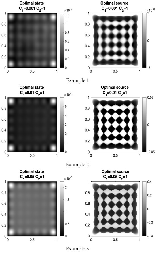
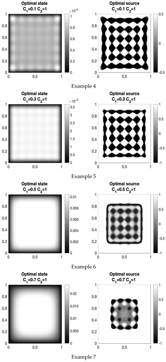
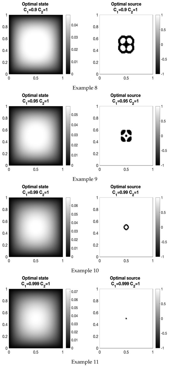Figure 1. Optimal state and control plots corresponding to examples 1–11.

The numerical details concerning each case are summarized in Table 1:

Table 1. For each of the examples, denoted here by ex 1–11, the number of iterations, the minimum compliance value, and a decay criterion in $L^2$ are provided.

Example	${\mathit{C}}_1$	Iter	Min	$\mathit{DSource}$	$\mathit{DState}$
ex 1	$0.001$	114	$2.9338\times {10}^{-9}$	$2.9478\times {10}^{-8}$	$9.4762\times {10}^{-16}$
ex 2	$0.01$	119	$2.8634\times {10}^{-9}$	$2.8105\times {10}^{-6}$	$8.5020\times {10}^{-14}$
ex 3	$0.05$	206	$3.8893\times {10}^{-6}$	$3.2343\times {10}^{-5}$	$9.8829\times {10}^{-13}$
ex 4	$0.1$	133	$3.6519\times {10}^{-5}$	$2.6914\times {10}^{-4}$	$8.9100\times {10}^{-12}$
ex 5	$0.3$	337	$5.9836\times {10}^{-4}$	$3.2096\times {10}^{-4}$	$9.0663\times {10}^{-11}$
ex 6	$0.5$	569	$3.2\times {10}^{-3}$	$1.4188\times {10}^{-4}$	$9.9691\times {10}^{-11}$
ex 7	$0.7$	406	$9.7\times {10}^{-3}$	$1.2890\times {10}^{-4}$	$9.9789\times {10}^{-11}$
ex 8	$0.9$	195	$2.34\times {10}^{-2}$	$2.4270\times {10}^{-4}$	$8.8048\times {10}^{-12}$
ex 9	$0.95$	68	$2.87\times {10}^{-2}$	$8.8752\times {10}^{-4}$	$5.9938\times {10}^{-12}$
ex 10	$0.99$	21	$3.38\times {10}^{-2}$	$2.5\times {10}^{-3}$	$9.9680\times {10}^{-12}$
ex 11	$0.999$	6	$3.51\times {10}^{-2}$	$1.3\times {10}^{-3}$	$1.5993\times {10}^{-12}$

Here, iter denotes the number of iterations performed, and min is the minimum value attained by the compliance. Despite the fact that our fundamental purpose has not been the development of a high-efficiency algorithm, the convergence is accomplished and is very fast. To ascertain that, we have considered as a criterion to guarantee the convergence to the optimal pair, the zero decay in the $L^2$ norms

$$DSource={∥f_{iter}-f_{iter-1}∥}_{L^2} \mathrm{and} DState={∥u_{f_{iter}}-u_{f_{iter-1}}∥}_{L^2}.$$

Compared with other algorithms for nonlocal optimal control problems, such as the projected gradient method used in [21], our method attains comparable accuracy with significantly reduced implementation complexity. In particular, avoiding adjoint computations and using a step-size selection based on monotonicity, we reduce the cost of each iteration. These features make the proposed approach especially suitable for large-scale simulations and for applications that require fast prototyping of the control structure.

We want to remark that although our theoretical analysis covers the nonlinear case $p\ne 2$ and establishes the convergence of the descent method in that setting, we restrict the numerical experiments to the laplacian case. The implementation of nonlinear exponents in nonlocal models entails additional numerical challenges, mainly related to the evaluation of nonlocal integrals and the interplay between the discretization parameters and the horizon $\delta$. Addressing these aspects requires developments that go beyond the scope of the present paper. A detailed numerical study for $p\ne 2$ will therefore be analyzed in a forthcoming work.

References

- Cea, J.; Malanowski, K. An example of a Max-Min problem in Partial Differential Equations. SIAM J. Control 1970, 8, 305–316. [Google Scholar] [CrossRef]
- Muñoz, J. Local and Nonlocal Optimal Control in the Source. Mediterr. J. Math. 2022, 19, 27. [Google Scholar] [CrossRef]
- Allaire, G. Shape Optimization by the Homogenization Method; Springer: New York, NY, USA, 2002. [Google Scholar]
- Bendsoe, M.P. Optimization fo Structural Topology, Shape, and Material; Springer: Berlin/Heidelberg, Germany, 1995. [Google Scholar]
- Bendsoe, M.P.; Sigmund, O. Topology Optimization: Theory, Methods, and Applications; Springer Science & Business Media: Berlin/Heidelberg, Germany, 2013. [Google Scholar]
- Topics in Mathematical Modeling of Composite Materials; Cherkaev, A., Kohn, R., Eds.; Birkhauser: Boston, MA, USA, 1997. [Google Scholar]
- Du, Q. Nonlocal Modeling, Analysis and Computation; Volume 94 of CBMS-NSF regional conference series in applied mathematics; SIAM: Philadelphia, PA, USA, 2019. [Google Scholar]
- Delfour, M.C.; Zolésio, J.P. Shapes and Geometries: Metrics, Analysis, Differential Calculus; Advances in Design and Control Series; SIAM: Philadelphia, PA, USA, 2011. [Google Scholar]
- Jikov, V.V.; Kozlov, S.M.; Oleinik, O.A. Homogenization of Differential Operators and Integral Functionals; Springer: Berlin/Heidelberg, Germany, 1994. [Google Scholar]
- Lions, J.L. Optimal Control of Systems Governed by Partial Differential Equations; Springer: Berlin/Heidelberg, Germany; New York, NY, USA, 1971. [Google Scholar]
- Andreu-Vaillo, F.; Mazón, J.M.; Rossi, J.D.; Toledo-Melero, J.J. Nonlocal Diffusion Problems; Mathematical Surveys and Monographs; American Mathematical Society: Providence, RI, USA, 2010; Volume 165. [Google Scholar]
- Bucur, C.; Valdinoci, E. Nonlocal Diffusion and Applications; Lecture Notes of the Unione Matematica Italiana, Volume 20; Springer: Cham, Switzerland, 2016. [Google Scholar]
- Vázquez, J.L. Nonlinear Diffusion with Fractional Laplacian Operators. In Nonlinear Partial Differential Equations: The Abel Symposium 2010; Holden, H., Karlsen, K., Eds.; Springer: Berlin/Heidelberg, Germany, 2012; pp. 271–298. [Google Scholar]
- Vázquez, J.L. The Mathematical Theories of Diffusion: Nonlinear and Fractional Diffusion. In Nonlocal and Nonlinear Diffusions and Interactions: New Methods and Directions; Bonforte, M., Grillo, G., Eds.; Lecture Notes in Mathematics; Springer: Cham, Switzerland, 2017; Volume 2186, pp. 205–278. [Google Scholar]
- Delfour, M.C.; Zolésio, J.P. The Optimal Design Problem of Céa and Malanowski Revisited. In Optimal Design and Control. Progress in Systems and Control Theory; Borggaard, J., Burkardt, J., Gunzburger, M., Peterson, J., Eds.; Birkhäuser: Boston, MA, USA, 1995; Volume 19. [Google Scholar] [CrossRef]
- Andrés, F.; Muñoz, J. A type of nonlocal elliptic problem: Existence and approximation through a Galerkin-Fourier Method. SIAM J. Math. Anal. 2015, 47, 498–525. [Google Scholar] [CrossRef]
- Andrés, F.; Muñoz, J. Nonlocal optimal design: A new perspective about the approximation of solutions in optimal design. J. Math. Anal. Appl. 2015, 429, 288–310. [Google Scholar] [CrossRef]
- Andrés, F.; Muñoz, J.; Rosado, J. Optimal design problems governed by the nonlocal p -Laplacian equation. Math. Control Relat. Fields 2021, 11, 119–141. [Google Scholar] [CrossRef]
- Andreu, F.; Rossi, J.D.; Toledo-Melero, J.J. Local and nonlocal weighted p-Laplacian evolution equations with Neumann boundary conditions. Publ. Mat. 2011, 55, 27–66. [Google Scholar] [CrossRef]
- Bellido, J.C.; Mora-Corral, C.; Pedregal, P. Hyperelastticity as a Γ-limit of Peridynamics when the horizon goes to zero. Cal. Var. 2015, 54, 1643–1670. [Google Scholar] [CrossRef]
- D’Elia, M.; Gunzburger, M. Optimal distributed control of nonlocal steady diffusion problems. SIAM J. Control Optim. 2014, 52, 243–273. [Google Scholar] [CrossRef]
- D’Elia, M.; Gunzburger, M. Identification of the diffusion parameter in nonlocal steady diffusion problems. Appl. Math. Optim. 2016, 73, 227–249. [Google Scholar] [CrossRef]
- Mengesha, T.; Du, Q. On the variational limit of a class of nonlocal functionals related to peridynamics. Nonlinearity 2015, 28, 3999–4035. [Google Scholar] [CrossRef]
- Mengesha, T.; Du, Q. Characterization of function spaces of vector fields and an application in nonlinear peridynamics. Nonlinear Anal. 2016, 140, 111. [Google Scholar] [CrossRef]
- Zhou, K.; Du, Q. Mathematical and numerical analysis of linear peridynamic models with nonlocal boundary conditions. SIAM J. Numer. Anal. 2010, 48, 1759–1780. [Google Scholar] [CrossRef]
- Aksoylu, B.; Mengesha, T. Results on nonlocal boundary value problems. Numer. Funct. Anal. Optim. 2010, 31, 1301–1317. [Google Scholar] [CrossRef]
- D’Elia, M.; Du, Q.; Gunzburger, M. Recent Progress in Mathematical and Computational Aspects of Peridynamics. In Handbook of Nonlocal Continuum Mechanics for Materials and Structures; Voyiadjis, G., Ed.; Springer: Cham, Switzerland, 2018. [Google Scholar] [CrossRef]
- Du, Q.; Gunzburger, M.D.; Lehoucq, R.B.; Zhou, K. Analysis and approximation of nonlocal Diffusion problems with volume constraints. SIAM Rev. 2012, 54, 667–696. [Google Scholar] [CrossRef]
- Hinds, B.; Radu, P. Dirichlet’s principle and wellposedness of solutions for a nonlocal p-Laplacian system. Appl. Math. Comput. 2012, 219, 1411–1419. [Google Scholar] [CrossRef]
- Antil, H.; Warma, M. Optimal control of the coefficient for the regional fractional p-Laplace equation: Approximation and convergence. Math. Control Relat. Fields 2019, 9, 1–38. [Google Scholar] [CrossRef]
- Bonder, J.F.; Spedaletti, J.F. Some nonlocal optimal design problems. J. Math. Anal. Appl. 2018, 459, 906–931. [Google Scholar] [CrossRef]
- Bellido, J.C.; Egrafov, A. A simple characterization of H-Convergence for a class of nonlocal problems. Rev. Mat. Complut. 2019, 34, 175–183. [Google Scholar] [CrossRef]
- Bonder, J.F.; Ritorto, A.; Martín, A. H-Convergence Result for Nonlocal Elliptic-Type Problems via Tartar’s Method. SIAM J. Math. Anal. 2017, 49, 2387–2408. [Google Scholar] [CrossRef]
- Ponce, A.C. A new approach to Sobolev Spaces and connections to Γ-convergence. Calc. Var. 2004, 19, 229–255. [Google Scholar] [CrossRef]
- Waurick, M. Nonlocal H-convergence. Calc. Var. Partial Differ. Equ. 2018, 57, 159. [Google Scholar] [CrossRef]
- Bourgain, J.; Brezis, H.; Mironescu, P. Another look at Sobolev spaces. In Optimal Control and Partial Differential Equations; Menaldi, J.L., Rofman, E., Sulem, A., Eds.; A Volume in Honour of A. Benssoussan’s 60th Birthday; IOS Press: Amsterdam, The Netherlands, 2001; pp. 439–455. [Google Scholar]
- Nezza, E.D.; Palatucci, G.; Valdinoci, E. Hitchhiker’s guide to the fractional Sobolev spaces. Bull. Sci. Math. 2012, 136, 521–573. [Google Scholar] [CrossRef]
- Mazón, J.M.; Rossi, J.D.; Toledo-Melero, J.J. Fractional p-Laplacian evolution equations. J. Math. Pures Appl. 2016, 105, 810–844. [Google Scholar] [CrossRef]
- Bonito, A.; Borthagaray, J.P.; Nochetto, R.H.; Otárola, E.; Salgado, A.J. Numerical Methods for fractional diffusion. arXiv 2017, arXiv:1707.01566v1. [Google Scholar] [CrossRef]
- Bonito, A.; Lei1, W.; Pasciak, J.E. Numerical approximation of the integral fractional Laplacian. Numer. Math. 2019, 142, 235–278. [Google Scholar] [CrossRef]
- Borthagaray, J.P.; Ciarlet, P. On the convergence in H1-norm for the fractional laplacian. arXiv 2018, arXiv:1810.07645v1. [Google Scholar]
- D’Elia, M.; Gunzburger, M. The fractional Laplacian operator on bounded domains as a special case of the nonlocal diffusion operator. arXiv 2013, arXiv:1303.6934v1. [Google Scholar] [CrossRef]
- Ciegis, R.; Starikovicius, V.; Margenov, S.; Kriauziene, R. Scalability analysis of differential parallel solvers for 3D fractional power diffusion problem. Concurr. Comput. 2019, 31, e5163. [Google Scholar] [CrossRef]
- Hao, Z.; Zhang, Z.; Du, R. Fractional Centered difference scheme for high-dimensional integral fractional Laplace. J. Comput. Phys. 2021, 424, 109851. [Google Scholar] [CrossRef]
- D’Elia, M.; Du, Q.; Glusa, C.; Gunzburger, M.; Tian, X.; Zhou, Z. Numerical methods for nonlocal and fractional models. arXiv 2020, arXiv:2002.01401. [Google Scholar] [CrossRef][Green Version]
- Andrés, F. Aproximación y Optimización de Problemas no Locales. Doctoral Dissertation, Universidad de Castilla-La Mnacha, Toledo, Spain, 2016. [Google Scholar]
- Evgrafov, A.; Bellido, J.C. Non local control in the conduction cefficients: Well posedness and convergence to the local limit. arXiv 2019, arXiv:1905.01931. [Google Scholar]
- Evgrafov, A.; Bellido, J.C. The nonlocal Kelvin principle and the dual approach to nonlocal control in the conduction coefficients. arXiv 2021, arXiv:2106.06031. [Google Scholar] [CrossRef]
- Brasco, L.; Parini, E.; Squassina, M. Stability fo variational eigenvalues for the fractional p-laplacian. arXiv 2015, arXiv:1503.04182v1. [Google Scholar]
- Teixeira, E.V.; Teymurazyan, R. Optimal design problems with fractional diffusions. J. Lond. Math. Soc. 2015, 92, 338–352. [Google Scholar] [CrossRef]
- Ponce, A.C. An estimate in the spirit of Poincaré’s inequality. J. Eur. Math. Soc. (JEMS) 2004, 6, 1–15. [Google Scholar] [CrossRef]
- Andrés, F.; Muñoz, J. On the convergence of a class of nonlocal elliptic equations and related optimal design problems. J. Optim. Theory Appl. 2017, 172, 33–55. [Google Scholar] [CrossRef]
- Muñoz, J. Generalized Ponce’s inequality. arXiv 2019, arXiv:1909.04146v2. [Google Scholar] [CrossRef]
- Chipot, M. Elliptic Equations: An Introductory Course; Birkhäuser: Cham, Switzerland, 2009. [Google Scholar]
Disclaimer/Publisher’s Note: The statements, opinions and data contained in all publications are solely those of the individual author(s) and contributor(s) and not of MDPI and/or the editor(s). MDPI and/or the editor(s) disclaim responsibility for any injury to people or property resulting from any ideas, methods, instructions or products referred to in the content. |
© 2025 by the authors. Licensee MDPI, Basel, Switzerland. This article is an open access article distributed under the terms and conditions of the Creative Commons Attribution (CC BY) license (https://creativecommons.org/licenses/by/4.0/).