A Least-Squares Control Strategy for Asymptotic Tracking and Disturbance Rejection Using Tikhonov Regularization and Cascade Iteration

Abstract

This paper presents a comprehensive strategy for addressing tracking and disturbance rejection for both lumped and distributed parameter systems, focusing on infinite-dimensional input and output spaces. Building on the geometric theory of regulation, the proposed methodology employs a cascade algorithm coupled with Tikhonov regularization to derive control laws that improve tracking accuracy iteratively. Unlike traditional optimal control approaches, the framework minimizes the limsup in time of the tracking error norm, rather than with respect to a quadratic cost function. It is important to note that this work also includes applicability to over- and under-determined systems. We provide theoretical insights, detailed algorithmic formulations, and numerical simulations to demonstrate the effectiveness and generality of the method. Results indicate that the cascade controls asymptotically approximate the classical optimal control solutions, with limitations addressed through rigorous error analysis. Applications include diverse scenarios with both finite and infinite-dimensional input and output spaces, showcasing the versatility of the approach.

1. Introduction

Tracking and disturbance rejection are fundamental objectives in control design, particularly for systems governed by partial differential equations (PDEs) [1,2,3]. This work presents a general strategy applicable to both lumped and distributed parameter systems, primarily focusing on systems modeled by PDEs. The proposed method generates a sequence of control laws by solving a cascade of easily manageable control problems. At each step, tracking accuracy is progressively enhanced through least-squares error minimization.

The foundation of the cascade algorithm, developed over a series of studies [4,5,6], lies in the theory of geometric regulation [1,7,8,9,10,11] and related works. Many of the authors’ previous studies have assumed finite-dimensional input and output spaces, with the additional constraint that the system transfer function at zero is invertible. A significant contribution of this work is the removal of such restrictions, enabling the algorithm to handle input and output spaces of arbitrary dimensionality. This generality allows the method to produce approximate controls even for infinite-dimensional input and output spaces and for over- or under-determined systems in the finite-dimensional case.

In this work, we do not claim that the resulting controls are optimal in the classical sense, as achieved through LQR or LQG methodologies [12,13], since we do not consider a quadratic time integral cost function. Instead, our goal is to generate suitable controls that enable the derivation of error estimates under straightforward smoothness assumptions and large-time supremum norm bounds for both the reference and disturbance signals. This approach accommodates extremely general signals that may have transient oscillations for a time but ultimately transition into smooth bounded motion. Most importantly, we do not require that these signals be generated by an exogenous system as in the classical theory.

In this work, we adopt a cost function based on the large-time supremum norm of the error rather than on an integral quadratic form. The resulting control algorithm is computationally efficient, simple to implement, and geared toward accurate long-term tracking and disturbance rejection. A notable advantage of this formulation is that the error at each step can be written in terms of explicit iterated convolution integrals (see [4,5,6]), which yield a priori estimates that may be computed offline. This perspective shifts the focus from traditional optimality to long-term performance, and it bears similarities to the discounted cost formulations used for infinite-horizon tracking problems [14].

Through several examples, we observe that the sequence of controls derived from the proposed algorithm converges in time to the classical optimal control solution. Here we note that standard optimal control problems for parabolic systems typically involve backward parabolic adjoint systems. Solving these problems often requires iterative forward–backward solutions or space–time discretization [15,16,17,18], which are computationally intensive. To alleviate this burden, approaches such as Receding-Horizon Control [19,20], ad hoc time-stepping schemes [21], and preconditioning techniques [22] have been proposed.

Finally, this study focuses on bounded input and output operators. However, the methodology can be extended to cases involving unbounded inputs and outputs, such as boundary control and sensing. Such generalizations require additional effort and will be addressed in future work.

The paper is organized as follows: Section 2 provides a statement of the problem, describing the plant as a controlled dynamical system with control inputs and outputs defined in an infinite-dimensional Hilbert space. The primary Control Objectives addressed in this work are formulated in Problems 1 and 2.

In Section 3, we present the approximate cascade controller. The initial step, referred to as the 0th-order controller, is given in (14) and (15), while the general jth-order controller is defined in (17) and (18). The motivation and derivation of the controller are discussed in Appendix A. Although not immediately apparent, this control strategy is rooted in obtaining approximate solutions to the regulator equations in the context of geometric regulation. Due to space limitations, details of the derivation process (e.g., $\beta$ regularization) are omitted here but thoroughly covered in prior works [1,4,5,6,23].

In Appendix A, Equation (A6), we present an initial form for the 0th-order controller and show why it is unsuitable. By substituting this control into equation (A1) and applying regularization and simplification, we obtain the final form (A17)–(A19), which leads to the results in (15).

At first glance, solving the dynamical systems in the controllers may seem numerically challenging. However, Section 4 presents a straightforward and practical algorithm for solving all cascade dynamical systems. This algorithm enables solutions using off-the-shelf finite element software, eliminating the need for complex numerical programming. In this section, we focus on the final results, leaving the detailed derivation of the Formulas (21)–(23) for the 0th-order equations and (25)–(27) for the jth-order equations to Appendix B.

A significant advantage of our control strategy is its ability to provide explicit formulas for the errors at each cascade step. These formulas express the errors in terms of the reference signals, disturbances, system parameters, the regularization parameter $\beta$, and the Tikhonov regularization parameter $\alpha$. In Section 5, we provide these explicit error formulas: (35) for the 0th step and (38) and (39) for the general nth-order step, where $n\ge 1$. As with the dynamical systems, the derivations of these results involve lengthy discussions, which are provided in Appendix D.

Section 6 presents a detailed analysis of the errors in the special case of finite-dimensional input and output spaces. In this scenario, sending the Tikhonov regularization parameter $\alpha$ to zero is possible, effectively replacing the Tikhonov regularization with the Moore–Penrose pseudoinverse. This approach enables a detailed examination of errors at each cascade step and an analysis of the overall cascade error structure. The ability to send $\alpha$ to zero critically depends on Lemma 1, whose proof is provided in Appendix C.

In Section 7, we consider a common situation in applications to partial differential equations with infinite-dimensional input and output spaces when the input map is given by an extension operator and the output map is given by a restriction operator. Here, the state operator A is a coercive elliptic operator acting in the state space $L^2\left(\mathrm{\Omega }\right)$, where $\mathrm{\Omega }$ is a bounded domain in ${\mathbb{R}}^n$, and the control input $u(x,t)$ acts on a subdomain ${\mathrm{\Omega }}_b\subset \mathrm{\Omega }$. In contrast, the output $y(x,t)$ corresponds to the solution of the differential equation evaluated on a subset ${\mathrm{\Omega }}_c\subset \mathrm{\Omega }$. Lemma 3 in Section 7 shows that in the case of infinite-dimensional input and output spaces, the only way one can achieve error zeroing is in the colocated case, i.e., ${\mathrm{\Omega }}_b={\mathrm{\Omega }}_c$.

In Section 8, we present numerical simulations covering a broad range of scenarios with both finite- and infinite-dimensional input/output spaces. Example 1 considers a two-input/two-output system, while Example 2 addresses an under-determined case where error zeroing fails. The remainder of our numerical examples are concerned with the most challenging case of infinite-dimensional input and output spaces. We then study a one-dimensional parabolic system with non-colocated input/output spaces (Example 3) and its colocated counterpart (Example 4). Finally, parabolic problems are examined in a two-dimensional spatial domain: a non-colocated case (Example 5) and a colocated case (Example 6).

As discussed above, many lengthy technical calculations have been moved to Appendix A, Appendix B, Appendix C, Appendix D and Appendix E to not detract from the main points in the paper.

2. Statement of Problem

We consider a control system with state operator A assumed to be sectorial with compact resolvent that generates an exponentially stable $C_0$ semigroup on the Hilbert space $\mathcal{Z}$ with inner product $⟨·,·⟩$ and norm $\parallel ·\parallel ={⟨·,·⟩}^{1/2}$. $B_{\mathrm{in}}:\mathcal{U}\to \mathcal{Z}$ is the bounded input operator, and $C:\mathcal{Z}\to \mathcal{Y}$ is the bounded output operator, where $\mathcal{U}$ and $\mathcal{Y}$ are the control input and output Hilbert spaces, respectively. Also, $B_{\mathrm{d}}:\mathcal{D}\to \mathcal{Z}$ is the bounded disturbance input operator, and $\mathcal{D}$ is the disturbance input space.

In this work, we emphasize that only bounded input, disturbance, and output operators are considered. However, after many numerical simulations, we have observed that the methodology presented here can be extended to cases involving unbounded inputs, disturbances, and outputs, such as boundary control and sensing. The analysis with such operators would require additional effort and will be addressed in future work.

Consider the control system in the Hilbert state space $\mathcal{Z}$

$$\begin{array}{cc}\hfill z_t& =Az+B_{\mathrm{d}}d+B_{\mathrm{in}}u,\hfill \end{array}$$

(1)

$$\begin{array}{cc}\hfill z\left(0\right)& =z_0,\hfill \end{array}$$

(2)

$$\begin{array}{cc}\hfill y\left(t\right)& =Cz\left(t\right).\hfill \end{array}$$

(3)

Problem 1.

Given a reference signal $r\in C_b^{\infty }({\mathbb{R}}^{+},\mathcal{Y})$ and disturbance $d\in C_b^{\infty }({\mathbb{R}}^{+},\mathcal{D})$ find a control u to minimize the limsup of the error, defined by $e\left(t\right)=r\left(t\right)-Cz\left(t\right)$. Namely, we want to minimize

$$\overline{\lim }{\parallel e\left(t\right)\parallel }_{\mathcal{Y}}.$$

(4)

Here, $C_b^{\infty }({\mathbb{R}}^{+},X)$ denotes the space of infinitely differentiable X-valued functions with all derivatives bounded on ${\mathbb{R}}^{+}$. More generally we will also consider $C_b^N({\mathbb{R}}^{+},X)$, the Banach space of smooth N-times continuously differentiable X-valued functions with all derivatives bounded on ${\mathbb{R}}^{+}$, and the notation $\overline{\lim }$ means

$$\overline{\lim }{\parallel \varphi \parallel }_X=\underset{T\to \infty }{lim}\underset{t\ge T}{sup}{\parallel \varphi \left(t\right)\parallel }_X,for\varphi \in C({\mathbb{R}}^{+},X).$$

It is desirable to choose the control $u\left(t\right)$ so that the error $e\left(t\right)=r\left(t\right)-Cz\left(t\right)$ vanishes asymptotically, which is often unachievable in classical optimal control.

We aim for a general setting, allowing $\mathcal{U}$ and $\mathcal{Y}$ to be either finite- or infinite-dimensional input and output spaces. In the case of infinite-dimensional input and output spaces, the problem becomes classically ill-posed, as the transfer function $G=C{(-A)}^{-1}{B}_{\mathrm{in}}$ is not boundedly invertible. In particular, G is a compact operator due to our assumptions on A, $B_{\mathrm{in}}$, and C; hence, it is non-invertible. Even in the finite-dimensional case, systems may be over- or under-determined, leading to additional challenges.

The Moore–Penrose pseudoinverse provides an ideal approximate control when available. However, it may not exist if the transfer function has a non-trivial null space or lacks a closed range. Such problems are generally challenging to solve, and solving for the control often leads to ill-posed inverse problems.

Therefore, to regularize the ill-posed problems, we employ Tikhonov regularization with a small penalty $\alpha >0$. The main theoretical problem we aim to address is the following.

Problem 2

(Control Objective). For the system (1)–(3), with given reference signals $r\in C_b^N({\mathbb{R}}^{+},\mathcal{Y})$ and disturbance $d\in C_b^N({\mathbb{R}}^{+},\mathcal{D})$, our objective is to choose a control u to minimize the limsup of the norm of the tracking error, $e\left(t\right)=r\left(t\right)-Cz\left(t\right)$.

Consider $\alpha >0$, and define

$$J_{\alpha }(z_0,r,d,u):=\overline{\lim }\left\{{\parallel e\parallel }_{\mathcal{Y}}^2+\alpha {\parallel u\parallel }_{\mathcal{U}}^2\right\}.$$

(5)

For given, $z_0$, r and d, our objective is to find u to minimize

$$\{J_{\alpha }\left(u\right):u\in \mathcal{S}\},$$

(6)

where $\mathcal{S}$ is the Constraint Set

$$\mathcal{S}=L^{\infty }(0,\infty ;\mathcal{U}).$$

(7)

A direct approach to Control Problem 2 results again in an ill-posed dynamical system. We introduce a second stabilization parameter $\beta \in (0,1)$ to regularize the system, producing an approximate control $u^0$. It is important to note that $u^0$ differs from u and may deviate significantly, potentially leading to an error $e_0$ larger than the desired e. This observation motivates the development of a cascade of control problems, where the Control Objective at each iteration is to reduce the error generated in the previous iteration, eventually converging to e.

The rationale and details behind the introduction of the regularization parameters $\alpha$ and $\beta$ are thoroughly explained in Appendix A. In the next section, we provide key definitions and a concise summary of the cascade controller algorithm described in Appendix A.

In the definition of the cost functional $J_{\alpha }$ in Problem 2, the parameter $\alpha$ has been taken as a scalar for simplicity. In a more general setting, $\alpha$ can be replaced by a symmetric positive definite weighting matrix $\mathit{A}$, thereby assigning distinct relative weights to the different control components or introducing cross-coupling between them. Analogously, a weighting matrix $\mathrm{\Gamma }$ can be introduced in the error norm to emphasize or de-emphasize specific components of the tracking error. In the infinite-dimensional framework, these ideas naturally extend to non-uniform weight functions or tensor-valued operators acting on the input and output spaces, allowing spatially varying or direction-dependent penalization. We emphasize that such matrix weights and non-uniform weighting functions can be seamlessly incorporated into the definition of the underlying norms, rendering the present formulation immediately extensible to these more general cases. In the remainder of the paper and in all numerical examples, we restrict attention to identity and uniform weights; however, this choice entails no loss of generality, and all theoretical results remain valid for the weighted case.

3. Approximate Cascade Controller

We begin by setting some notation. Denote by G the transfer function for A, $B_{\mathrm{in}}$, C evaluated at 0. Namely, $G:\mathcal{U}\to \mathcal{Y}$ is given by

$$G=C{(-A)}^{-1}{B}_{\mathrm{in}}.$$

(8)

Recall that if $\mathcal{U}$ and $\mathcal{Y}$ are infinite-dimensional, even if G is injective ($N\left(G\right)=\left\{0\right\}$), $G^{*}G$ has an unbounded inverse; thus, the Moore–Penrose pseudoinverse cannot be directly computed. Indeed, since $G^{*}G$ is a compact operator, the inverse is unbounded unless the input and output spaces are finite-dimensional. In what follows, the * notation refers to the Hilbert space adjoint operator. Definitions for the bounded case are in Chapter 2, page 31, and for the unbounded case in Chapter 10, page 305 [24]; see also T. Kato [25].

For $\alpha >0$, define

$$R_{\alpha }:={(\alpha I+G^{*}G)}^{-1}{G}^{*}:\mathcal{Y}\to \mathcal{U},$$

(9)

which forms the basis for applying Tikhonov regularization, as discussed in detail in [26,27,28,29,30]. Then, for $0<\beta <1$, define

$$R_{\alpha ,\beta }:={(\alpha I+\beta G^{*}G)}^{-1}{G}^{*}.$$

(10)

Next, we simplify the notation by defining

$$\begin{array}{cc}\hfill & B_{\alpha ,\beta }:=B_{\mathrm{in}}{R}_{\alpha ,\beta },\hfill \end{array}$$

(11)

$$\begin{array}{cc}\hfill & A_{\alpha ,\beta }:=A-(1-\beta )B_{\alpha ,\beta }C,\hfill \end{array}$$

(12)

$$\begin{array}{cc}\hfill & I_{\alpha ,\beta }:=I+\beta B_{\alpha ,\beta }C{A}^{-1}.\hfill \end{array}$$

(13)

A detailed discussion on the appropriate choice of $\beta$ will be provided later, ensuring that the operator $A_{\alpha ,\beta }$, as defined in (12), generates an exponentially stable analytic semigroup.

With the above notations, we can introduce the first step in the cascade controller given by the dynamical system

$$z_t^0=A_{\alpha ,\beta }{z}^0+I_{\alpha ,\beta }{B}_{\mathrm{d}}d\left(t\right)+B_{\alpha ,\beta }r\left(t\right),z^0\left(0\right)=z_0,$$

(14)

which produces the first approximate control

$$u^0\left(t\right)=R_{\alpha ,\beta }\left[r\left(t\right)-(1-\beta )C{z}^0+\beta C{A}^{-1}{B}_{\mathrm{d}}d\left(t\right)\right].$$

(15)

We then obtain the first approximate error

$$e_0\left(t\right)=r\left(t\right)-C{z}^0\left(t\right).$$

(16)

The derivation of the controller system in (14) and (15) is presented in Appendix A. We note that the controller (14) and (15) is a feedback (dynamic) controller that depends only on $r\left(t\right)$, $d\left(t\right)$, and $z_0$.

In general, the control $u^0$ will not be accurate enough to solve our tracking problem due to the effect of the $\beta$ regularization parameter. Therefore, we propose a sequence, or cascade, of controllers, where each stage improves the approximate control and reduces the error. Each stage solves a new approximate tracking problem, using the previous step’s error as the reference signal.

Namely, for a fixed $n\in {\mathbb{Z}}^{+}$ and $1\le j\le n$, define new variables $z^j$, $u^j$, and the jth cascade controller as follows.

$$z_t^j=A_{\alpha ,\beta }{z}^j+B_{\alpha ,\beta }{e}_{j-1}\left(t\right),z^j\left(0\right)=0,$$

(17)

which produces a new control law $u^j$ given by

$$u^j=R_{\alpha ,\beta }(e_{j-1}\left(t\right)-(1-\beta )C{z}^j),$$

(18)

and, this, in turn, will produce a new cascade error $e_j$ given by

$$e_j\left(t\right)=e_{j-1}\left(t\right)-C\left(z^j\right).$$

(19)

Furthermore, all the coefficients in the controllers (14) and (15), as well as (17) and (18), can be “precomputed” in terms of $R_{\alpha ,\beta }$, $\beta$, $B_{\mathrm{in}}$, C, $B_{\mathrm{d}}$, and $A^{-1}{B}_{\mathrm{d}}$.

The nth step cascade control used in the plant (1)–(3) is given by the sum

$$u_n=\sum _{j=0}^n{u}^j.$$

(20)

Since the initial conditions in (2) and (14) coincide and the semigroup generated by A is assumed to be exponentially stable, linearity implies that if the control $u_n$ is used in plant (1), then the state, z, and error $e\left(t\right)$ satisfy

$$z\left(t\right)=\sum _{j=0}^n{z}^j\left(t\right),\mathrm{and}e\left(t\right)=e_n\left(t\right)\mathrm{for}\mathrm{all}t\ge 0.$$

A key advantage of cascade controllers is that they enable a detailed analysis of the errors $e_j\left(t\right)$, leading to explicit formulas for the errors. For finite-dimensional input and output spaces, these formulas yield concise error estimates, as presented in Theorem 1.

Remark 1.

The term cascade here does not refer to the classical two-loop cascade control architecture used in process or networked control systems [31,32]. Instead, it denotes an iterative correction scheme in which each stage of the algorithm uses the tracking error from the previous stage as input, progressively refining the control and reducing the error within each cascade step.

4. A Practical Solution Algorithm for the Controllers

This section presents a simple algorithm for solving the dynamical systems (14) and (17). The primary difficulty lies in handling the expression $R_{\alpha ,\beta }$. One common approach is to use the Singular Value Decomposition (SVD) of the bounded linear operator $G^{*}G$. The SVD is useful for theoretical results. However, explicitly determining the singular values and corresponding eigenfunctions in the infinite-dimensional case is rarely feasible. Therefore, developing a numerical algorithm that can be implemented using standard off-the-shelf finite element software is advantageous.

Appendix B presents a procedure that leads to the following algorithm for solving (14) and obtaining $u^0$.

$$\begin{array}{cc}\hfill z_t^0=& A{z}^0+B_{\mathrm{d}}d+B_{\mathrm{in}}{B}_{\mathrm{in}}^{*}\left({\displaystyle \frac{X_0}{\alpha }}\right),\hfill \end{array}$$

(21)

$$\begin{array}{cc}\hfill 0=& A^{*}{X}_0+C^{*}\left(r-(1-\beta )C{z}^0-\beta C{Y}_0\right),\hfill \end{array}$$

(22)

$$\begin{array}{cc}\hfill 0=& A{Y}_0+B_{\mathrm{d}}d+B_{\mathrm{in}}{B}_{\mathrm{in}}^{*}\left({\displaystyle \frac{X_0}{\alpha }}\right),\hfill \end{array}$$

(23)

where the approximate control $u^0$ is given by

$$u^0=B_{\mathrm{in}}^{*}\left({\displaystyle \frac{X_0}{\alpha }}\right).$$

(24)

Similarly, for the systems (17) with control (18), we have

$$\begin{array}{cc}\hfill z_t^j=& A{z}^j+B_{\mathrm{in}}{B}_{\mathrm{in}}^{*}\left({\displaystyle \frac{X_j}{\alpha }}\right),\hfill \end{array}$$

(25)

$$\begin{array}{cc}\hfill 0=& A^{*}{X}_j+C^{*}\left(e_{j-1}-(1-\beta )C{z}^j-\beta C{Y}_j\right),\hfill \end{array}$$

(26)

$$\begin{array}{cc}\hfill 0=& A{Y}_j+B_{\mathrm{in}}{B}_{\mathrm{in}}^{*}\left({\displaystyle \frac{X_j}{\alpha }}\right),\hfill \end{array}$$

(27)

where the approximate cascade controls $u^j$ are given by

$$u^j=B_{\mathrm{in}}^{*}\left({\displaystyle \frac{X_j}{\alpha }}\right).$$

(28)

Finally, the nth step control to be used in the plant is given by

$$u_n={\displaystyle \frac{B_{\mathrm{in}}^{*}}{\alpha }}\sum _{j=0}^n{X}_j.$$

(29)

At each cascade level, we solve one parabolic PDE for $z^i(x,t)$ together with the constraint equations for the coupled fields $(X^i(x,t),Y^i(x,t))$. Although $X^i$ and $Y^i$ lack explicit time derivatives, they are algebraically coupled to $z^i(x,t)$ and are computed simultaneously via standard time marching from $t^{k-1}$ to $t^k$. We implemented this on several platforms, including COMSOL Multiphysics 6.1, and in-house FEM software (MATLAB R2025b, and FEMuS, available on GitHub, https://github.com/eaulisa/MyFEMuS, accessed on 11 November 2025), all showing similar behavior; all reported results in Section 7 use COMSOL and their implementation is basic. A detailed scheme is given in Figure 1. Unlike classical optimal control with a backward-in-time parabolic adjoint equation over $[0,T]$ [17,18], our scheme advances only forward, simplifying computation.

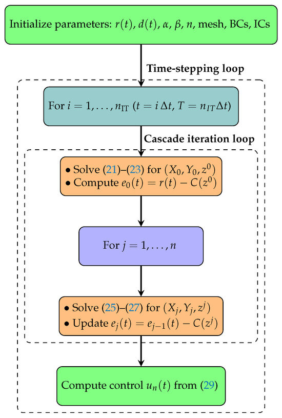
Figure 1. Block diagram of the solution algorithm for the cascade controller in the time interval $(0,T]$. The outer loop advances in time, while the inner loop iterates over the cascade index j.

5. Explicit Formulas for the Errors

The analysis of the error $e_0\left(t\right)$ is carried out in Appendix D by applying the variation of parameters formula to the dynamical system (14), followed by integration by parts.

Define the operator

$$L_{\alpha }:=(I-G{R}_{\alpha }),$$

(30)

where $R_{\alpha }$ is defined in (9). Denote by L the orthogonal projection of the output space $\mathcal{Y}$ onto the null space of $G{G}^{*}$, $N\left(G{G}^{*}\right)=N\left(G^{*}\right)=R{\left(G\right)}^{\perp }$. Then, $(I-L)$ is the orthogonal projection onto the $\overline{R\left(G\right)}$ and $I=L+(I-L)$. Using this orthogonal decomposition, it follows that $L_{\alpha }$ can be written as

$$L_{\alpha }=L+M_{\alpha },M_{\alpha }:=\alpha {(\alpha I+G{G}^{*})}^{-1}(I-L).$$

(31)

Notice that

$$\mathcal{Y}=N\left(G^{*}\right)\oplus \tilde{\mathcal{Y}}\mathrm{where}\tilde{\mathcal{Y}}=(I-L)\mathcal{Y}.$$

The key properties of the operator $M_{\alpha }:\mathcal{Y}\to \mathcal{Y}$ are contained in the following lemma.

Lemma 1.

Recall our formula for $M_{\alpha }$ from (31). For any $\psi \in \mathcal{Y}$ (whether $\mathcal{Y}$ is finite or infinite-dimensional), we have $(I-L)\psi \in \tilde{\mathcal{Y}}$, and

$$\underset{\alpha \to 0}{lim}{M}_{\alpha }\psi =0.$$

In the case where the number of inputs and outputs is finite, we can say more. Namely, there exists ${\sigma }_c>0$ such that

$$\parallel M_{\alpha }\parallel \le {\displaystyle \frac{\sqrt{\alpha }}{2{\sigma }_c}},$$

(32)

so that $M_{\alpha }$ converges to zero in the operator norm as $\alpha \to 0$.

The proof of Lemma 1 is provided in Appendix C.

Let us define

$$K\left(t\right):=C{(-A_{\alpha ,\beta })}^{-1}{e}^{A_{\alpha ,\beta }t}{B}_{\alpha ,\beta },K_d\left(t\right):=C{(-A_{\alpha ,\beta })}^{-1}{e}^{A_{\alpha ,\beta }t}{I}_{\alpha ,\beta }{B}_{\mathrm{d}},$$

(33)

and

$$S_0:=I,S_i:=\left(M_{\alpha }+K\ast {\displaystyle \frac{d}{dt}}\right)S_{i-1}={\left(M_{\alpha }+K\ast {\displaystyle \frac{d}{dt}}\right)}^i,i\in {\mathbb{Z}}^{+}.$$

(34)

Note that the operators $M_{\alpha }$ and ${\displaystyle K\ast \frac{d}{dt}}$ do not commute. Nevertheless, employing the formulas presented in Appendix D, we can write

$$\begin{array}{cc}\hfill e_0\left(t\right)& =P\left(t\right)+L_{\alpha }\left(r\left(t\right)+C{A}^{-1}{B}_{\mathrm{d}}d\left(t\right)\right)+(K\ast r^{\prime })\left(t\right)+(K_d\ast d^{\prime })\left(t\right)\hfill \\ \hfill & =P\left(t\right)+\left[L_{\alpha }r\left(t\right)+(K\ast r^{\prime })\left(t\right)\right]+\left[L_{\alpha }C{A}^{-1}{B}_{\mathrm{d}}d\left(t\right)+(K_d\ast d^{\prime })\left(t\right)\right]\hfill \\ \hfill & =P\left(t\right)+\left[(L+S_1)r\left(t\right)\right]+\left[L_{\alpha }C{A}^{-1}{B}_{\mathrm{d}}d\left(t\right)+(K_d\ast d^{\prime })\left(t\right)\right]\hfill \\ \hfill & =e_0^r\left(t\right)+e_0^d\left(t\right),\hfill \end{array}$$

(35)

with

$$\begin{array}{cc}\hfill e_0^r\left(t\right)& :=P\left(t\right)+(L+S_1)r\left(t\right)\hfill \end{array}$$

(36)

$$\begin{array}{cc}\hfill e_0^d\left(t\right)& :=P\left(t\right)+L_{\alpha }C{A}^{-1}{B}_{\mathrm{d}}d\left(t\right)+(K_d\ast d^{\prime })\left(t\right)\hfill \end{array}$$

(37)

Here and in the future, $P\left(t\right)$ denotes a generic exponentially decaying function that depends on initial data and other known variables. At each iteration, $P\left(t\right)$ may change, but for simplicity, we do not track these changes and redefine $P\left(t\right)$ accordingly.

From (35), we note that the operator $L_{\alpha }=I-G{R}_{\alpha }$ in (30) plays a central role in the error $e_0\left(t\right)$, as well as in the errors $e_n\left(t\right)$ for $n\ge 1$. Appendix D, specifically Lemmas A2 and A3, contains the derivation of the following expressions for $e_n\left(t\right)$. For all $n\ge 1$, we have

$$e_n\left(t\right)=e_n^r\left(t\right)+e_n^d\left(t\right),$$

with

$$\begin{array}{cc}\hfill e_n^r\left(t\right)& =P\left(t\right)+\left(L\sum _{p=0}^n{S}_p+S_{n+1}\right)r\left(t\right),\hfill \end{array}$$

(38)

$$\begin{array}{cc}\hfill e_n^d\left(t\right)& =P\left(t\right)+\left(L\sum _{p=0}^{n-1}{S}_p+S_n\right)e_0^d\left(t\right).\hfill \end{array}$$

(39)

Since $L{M}_{\alpha }=0$ (cf. Remark A1 in Appendix D), it is possible to rewrite the generic Formulas (38) and (39) using the following relation:

$$L{S}_i=L\left(M_{\alpha }+K\ast {\displaystyle \frac{d}{dt}}\right)S_{i-1}=L\left(K\ast {\displaystyle \frac{d}{dt}}{S}_{i-1}\right),\forall i\in {\mathbb{Z}}^{+}.$$

6. Error Estimates for Finite-Dimensional Input and Output Spaces

For Problem 1, Tikhonov regularization, as described in Appendix A, is not the only potential optimization method. An alternative approach could involve a least-squares minimal solution using the Moore–Penrose pseudoinverse. However, Tikhonov regularization appears to be the better choice in control systems governed by partial differential equations and with infinite-dimensional input and output spaces $\mathcal{U}$ and $\mathcal{Y}$. For finite-dimensional $\mathcal{U}$ and $\mathcal{Y}$, which are common in many applications, it is useful to assess the impact on Section 3, since G then yields a simpler formula for $R_{\alpha }$, as defined in (9).

From (9), assuming $\left(G^{*}G\right)$ is invertible, as $\alpha \to 0$, we have

$$\underset{\alpha \to 0}{lim}{R}_{\alpha }={\left(G^{*}G\right)}^{-1}{G}^{*}:=G^{†},$$

where $G^{†}$ denotes the Moore–Penrose pseudoinverse. According to Lemma 1, $\parallel M_{\alpha }\parallel \to 0$ as $\alpha \to 0$, so $L_{\alpha }=L+M_{\alpha }$, defined in (31), converges to L.

Our main goal in this section is to estimate $\overline{\lim }\parallel e_n\left(t\right)\parallel$. To this end, assuming that we have passed $\alpha$ to zero, let us define

$${\overline{e}}_n\left(t\right):={\overline{e}}_n^r\left(t\right)+{\overline{e}}_n^d\left(t\right)=\underset{\alpha \to 0}{lim}{e}_n^r\left(t\right)+\underset{\alpha \to 0}{lim}{e}_n^d\left(t\right),$$

(40)

with $e_n^r\left(t\right)$ defined in (38) and $e_n^d\left(t\right)$ defined in (39). In Appendix E, Equation (A68), we show that

$$\begin{array}{cc}\hfill {\overline{e}}_n=\underset{\alpha \to 0}{lim}(e_n^r+e_n^d)& =P+L\left(\sum _{j=0}^n{(K\ast )}^j{r}^{\left(j\right)}+C{A}^{-1}{B}_{\mathrm{d}}d+\sum _{j=1}^n{(K\ast )}^{j-1}{K}_d\ast d^{\left(j\right)}\right)\hfill \\ \hfill & +{(K\ast )}^{n+1}{r}^{(n+1)}+{(K\ast )}^n{K}_d\ast d^{(n+1)}.\hfill \end{array}$$

(41)

For $j\ge 1$, define

$${\mathcal{H}}_0\left(t\right)=r\left(t\right)+C{A}^{-1}{B}_{\mathrm{d}}d\left(t\right)\mathrm{and}{\mathcal{H}}_j\left(t\right)={(K\ast )}^j{r}^{\left(j\right)}\left(t\right)+{(K\ast )}^{j-1}{K}_d\ast d^{\left(j\right)}\left(t\right),$$

(42)

and then the error ${\overline{e}}_n\left(t\right)$ can be written explicitly as

$${\overline{e}}_n\left(t\right):=P\left(t\right)+L\left(\sum _{j=0}^n{\mathcal{H}}_j\left(t\right)\right)+{\mathcal{H}}_{n+1}\left(t\right).$$

(43)

Remark 2.

In deriving the error formula (43) for $\alpha \to 0$, we have not explicitly included the dependence of the operators K and $K_d$ on α. Explicit formulas for these operators are provided later in Equation (47) and Theorem 1.

In the case of finite-dimensional input and output spaces, the projection operator L takes the form

$$L=(I-G{G}^{†})=(I-G{\left(G^{*}G\right)}^{-1}{G}^{*}),$$

(44)

and we have

$$G^{†}(I-G{G}^{†})=(G^{†}-G^{†})=0.$$

Remark 3.

One important special case occurs when $n_b=n_c$ and G is invertible. In this case

$$G^{†}={\left(G^{*}G\right)}^{-1}{G}^{*}=G^{-1}{\left(G^{*}\right)}^{-1}{G}^{*}=G^{-1}.$$

This case has been treated in detail in the earlier works [1,4,5,6] and references therein. In particular, the steps required to compute the limsup of the norms of the iterated errors described below are not repeated here; rather, we refer to these works for the specific details. A critical observation in the case G is invertible is that

$$L=(I-G{G}^{†})=(I-G{G}^{-1})=0.$$

As a result, in this case, it can be shown that the controls obtained from the iterative process are always error zeroing.

Considering the more general analysis of the errors in the case of finite-dimensional input and output spaces, we now estimate

$$\overline{\lim }\parallel {\overline{e}}_n\left(t\right)\parallel \le \overline{\lim }\parallel {\overline{e}}_n^r\left(t\right)\parallel +\overline{\lim }\parallel {\overline{e}}_n^d\left(t\right)\parallel .$$

For both ${\overline{e}}_n^r\left(t\right)$ and ${\overline{e}}_n^d\left(t\right)$, estimates of these expressions require estimating the limsup of iterated convolutions. This procedure has already been addressed, and the interested reader can consult [1,4,5,6,23]. Here, we present only the essential results.

Definition 1.

For $I\subseteq {\mathbb{R}}^{+}$, a fixed interval, the space $C_b^N(I,\mathbb{R})$, consisting of real-valued functions that are N-times continuously differentiable on I and whose derivatives up to order N are bounded, is a Banach space with the norm

$${\parallel \phi (·)\parallel }_{I,N}=\underset{0\le j\le N}{max}\left(\underset{t\in I}{sup}\left|{\phi }^{\left(j\right)}\left(t\right)\right|\right).$$

In the vector-valued case, let $\phi (·)={[{\phi }_1(·),{\phi }_2(·),\dots ,{\phi }_m(·)]}^T$ so that $\phi (·)\in C_b^N(I,{\mathbb{R}}^m)$. We define its norm by

$${\parallel \phi (·)\parallel }_{I,N}=\underset{1\le i\le m}{sup}(\parallel {\phi }_i(·){\parallel }_{I,N}).$$

For any interval $I\subset {\mathbb{R}}^{+}$, the reference $r(·)$ and disturbance $d(·)$ signals are smooth, bounded, vector-valued functions in $C_b^N(I,\mathcal{Y})$ and $C_b^N(I,\mathcal{D})$, respectively. We also note that for any $0\le j<N$

$$\begin{array}{c}\hfill {\parallel r\parallel }_{I,j}\le {\parallel r\parallel }_{I,j+1}\le {\parallel r\parallel }_{I,N}{and\parallel d\parallel }_{I,j}\le {\parallel d\parallel }_{I,j+1}\le {\parallel d\parallel }_{I,N}.\end{array}$$

(45)

Remark 4.

In establishing our estimates for the limsup of the errors, we are particularly interested in the supremum norm taken over time intervals of the form $I=[T,\infty )$ for a large $T>0$. This allows us to consider reference and disturbance signals that may have large excursions for some time but eventually settle into a more stable oscillatory behavior. To simplify the notation in this case, we write

$$\overline{\lim }{\parallel \phi (·)\parallel }_N=\underset{T\to \infty }{lim}{\parallel \phi (·)\parallel }_{[T,\infty ),N}.$$

(46)

To describe the error estimates in the special case considered in this section, we also need the form of various operators as $\alpha \to 0$. From (12), we have

$$\underset{\alpha \to 0}{lim}{A}_{\alpha ,\beta }=\underset{\alpha \to 0}{lim}\left(A-(1-\beta )B_{\mathrm{in}}{(\alpha I+\beta G^{*}G)}^{-1}{G}^{*}C\right)=A-{\displaystyle \frac{(1-\beta )}{\beta }}{B}_{\mathrm{in}}{G}^{†}C,$$

and from (13), we have

$$\underset{\alpha \to 0}{lim}{I}_{\alpha ,\beta }=\underset{\alpha \to 0}{lim}\left(I+\beta B_{\mathrm{in}}{(\alpha I+\beta G^{*}G)}^{-1}{G}^{*}C{A}^{-1}\right)=I+B_{\mathrm{in}}{G}^{†}C{A}^{-1}.$$

This leads to the definitions

$$A_{\beta }:=A-{\displaystyle \frac{(1-\beta )}{\beta }}{B}_{\mathrm{in}}{G}^{†}C,I_0:=I+B_{\mathrm{in}}{G}^{†}C{A}^{-1}.$$

(47)

Using these formulas, we obtain the form of $K\left(t\right)$ and $K_d\left(t\right)$ for $\alpha =0$ given in (48), in the following theorem.

Theorem 1.

Let

$$K\left(t\right)=-{\displaystyle \frac{1}{\beta }}C{A}_{\beta }^{-1}{e}^{A_{\beta }t}{B}_{\mathrm{in}},K_d\left(t\right)=-C{A}_{\beta }^{-1}{e}^{A_{\beta }t}{I}_0{B}_{\mathrm{d}},$$

(48)

where $A_{\beta }$ and $I_0$ are given in (47), and set

$$D={\int }_0^{\infty }\parallel K\left(t\right)\parallel \mathrm{d}t,D_d={\int }_0^{\infty }\parallel K_d\left(t\right)\parallel \mathrm{d}t.$$

(49)

For any $N\ge 0$ and any reference and disturbance signals, $r(·)\in C_b^N({\mathbb{R}}^{+},{\mathbb{R}}^{n_b}),andd(·)\in C_b^N({\mathbb{R}}^{+},{\mathbb{R}}^{n_c})$, define

$$\mathfrak{D}={\displaystyle \frac{D_d}{D}},C_N=\left(\overline{\lim }{\parallel r\parallel }_N+\mathfrak{D}\overline{\lim }{\parallel d\parallel }_N\right).$$

(50)

Then, we have

$$\overline{\lim }\parallel {\mathcal{H}}_N\left(t\right)\parallel \le D^N{C}_N.$$

(51)

Proof. 

Using the definition of ${\mathcal{H}}_N$ in (42), we have

$$\begin{array}{cc}\hfill \overline{\lim }\parallel {\mathcal{H}}_N\left(t\right)\parallel & \le \overline{\lim }{\parallel (K\ast )}^N{r}^{\left(N\right)}\left(t\right)\parallel +\overline{\lim }\parallel {(K\ast )}^{N-1}{K}_d\ast d^{\left(N\right)}\left(t\right)\parallel \hfill \\ \hfill & \le D^N\overline{\lim }{\parallel r\parallel }_N+D^{N-1}{D}_d\overline{\lim }{\parallel d\parallel }_N\hfill \\ \hfill & =D^N{C}_N.\hfill \end{array}$$

The proof that

$$\overline{\lim }{\parallel (K\ast )}^N{r}^{\left(N\right)}\left(t\right)\parallel \le D^N\overline{\lim }{\parallel r\parallel }_N\mathrm{and}\overline{\lim }{\parallel (K\ast )}^{N-1}{K}_d\ast d^{\left(N\right)}\left(t\right)\parallel \le D^{N-1}{D}_d\overline{\lim }{\parallel d\parallel }_N$$

involves a lengthy series of calculations involving estimates of repeated convolution integrals. The details of this analysis can be found in [5]. □

A frequently encountered case in the analysis of tracking and disturbance rejection of sinusoidal signals leads directly to the following corollary.

Corollary 1.

For reference signal $r(·)$ and disturbance $d(·)$, assume that there exist constants $\delta >0$, $\overline{C}>0$ such that

$$M_N=max\left(\overline{\lim }{\parallel r\parallel }_N,\overline{\lim }{\parallel d\parallel }_N\right)\le \overline{C}{\delta }^N\mathrm{with}\delta D<1,$$

for all $N\in {\mathbb{Z}}^{+}$. Then

$$C_N\le (1+\mathfrak{D})\overline{C}{\delta }^N,$$

and for sufficiently large N, we have

$$\overline{\lim }\parallel {\mathcal{H}}_N\parallel \le \overline{C}(1+\mathfrak{D}){\left(D\delta \right)}^N.$$

(52)

Therefore, from (43), we have

$$\underset{n\to \infty }{lim}\overline{\lim }∥{\overline{e}}_n∥=\overline{\lim }∥L\left(\sum _{j=0}^{\infty }{\mathcal{H}}_j\right)∥,$$

where the infinite sum converges due to the geometric convergence of ${\mathcal{H}}_j$. Furthermore, in the special case that $G^{†}=G^{-1}$, so that $L=0$, we see that the problem is “error zeroing”, i.e.,

$$\underset{n\to \infty }{lim}\overline{\lim }\parallel {\overline{e}}_n\parallel =0.$$

In particular, we have from (52)

$$\overline{\lim }\parallel {\overline{e}}_n\left(t\right)\parallel =\overline{\lim }\parallel {\mathcal{H}}_{n+1}(·)\parallel \le (1+\mathfrak{D}){\left(D\delta \right)}^{n+1}\stackrel{n\to \infty }{\to }0.$$

7. Infinite-Dimensional Colocated Input and Output Spaces

A reasonably general situation with infinite-dimensional input and output spaces arises in the control of partial differential equations defined on a bounded domain $\mathrm{\Omega }\subset {\mathbb{R}}^n$, with state space $\mathcal{Z}=L^2\left(\mathrm{\Omega }\right)$. In this case, the operator A is often a coercive elliptic operator with smooth coefficients. We assume that the control $u=u(x,t)$ acts through a subdomain ${\mathrm{\Omega }}_b\subseteq \mathrm{\Omega }$, while the measured output is taken on another subdomain ${\mathrm{\Omega }}_c\subseteq \mathrm{\Omega }$. The control operator $B_{\mathrm{in}}$ maps the input space $\mathcal{U}=L^2\left({\mathrm{\Omega }}_b\right)$ to the state space $\mathcal{Z}=L^2\left(\mathrm{\Omega }\right)$ and the measured output operator maps $\mathcal{Z}=L^2\left(\mathrm{\Omega }\right)$ to the output space $\mathcal{Y}=L^2\left({\mathrm{\Omega }}_c\right)$. In our examples involving infinite-dimensional input and output spaces, we will use the following operators to facilitate the definition of the input and output maps.

Definition 2.

Let ${\mathrm{\Omega }}_a\subset \mathrm{\Omega }$. Then, we define

1. 

Restriction Operator ${\mathcal{R}}_a:L^2\left(\mathrm{\Omega }\right)\to L^2\left({\mathrm{\Omega }}_a\right)$ is defined for $\phi \in L^2\left(\mathrm{\Omega }\right)$ by

$${\mathcal{R}}_a\phi \left(x\right)=\phi \left(x\right)\mathrm{for}x\in {\mathrm{\Omega }}_a.$$

(53)

Or, more simply ${\displaystyle {\mathcal{R}}_a{\phi \left(x\right)=\phi \left(x\right)|}_{x\in {\mathrm{\Omega }}_a}}$.

2. 

Extension Operator ${\mathcal{E}}_a:L^2\left({\mathrm{\Omega }}_a\right)\to L^2\left(\mathrm{\Omega }\right)$ is defined for $\psi \in L^2\left({\mathrm{\Omega }}_a\right)$ by

$${\mathcal{E}}_a\psi \left(x\right)=\left\{\begin{array}{cc}\psi \left(x\right),\hfill & x\in {\mathrm{\Omega }}_a\hfill \\ 0,\hfill & x\in \mathrm{\Omega }\setminus {\mathrm{\Omega }}_a\hfill \end{array}\right..$$

(54)

Using these definitions, for $\phi \in L^2\left({\mathrm{\Omega }}_b\right)$, we can write

$$B_{\mathrm{in}}\phi \left(x\right)={\mathcal{E}}_b\phi \left(x\right).$$

(55)

Similarly, for $\psi \in \mathcal{Z}$, define

$$C\psi \left(x\right)={\mathcal{R}}_c\psi \left(x\right).$$

(56)

In addition, we define $B_{\mathrm{d}}:L^2\left({\mathrm{\Omega }}_d\right)\to L^2\left(\mathrm{\Omega }\right)$ for $\phi \in L^2\left({\mathrm{\Omega }}_d\right)$ by

$$B_{\mathrm{d}}\phi \left(x\right)={\mathcal{E}}_d\phi \left(x\right).$$

(57)

Then, the operators $B_{\mathrm{in}}$, $B_{\mathrm{d}}$, and C are bounded operators from their respective domains to their range spaces. Similarly, for the adjoint operators, we have

$$B_{\mathrm{in}}^{*}\psi \left(x\right)={\mathcal{R}}_b\psi \left(x\right),$$

(58)

$$C^{*}\phi \left(x\right)={\mathcal{E}}_c\phi \left(x\right).$$

(59)

In this case, we can easily express a formula for the operators G and $G^{*}$ as

$$\begin{array}{cc}\hfill G& =C{(-A)}^{-1}{B}_{\mathrm{in}}:L^2\left({\mathrm{\Omega }}_b\right)\to L^2\left({\mathrm{\Omega }}_c\right),\hfill \\ \hfill G^{*}& =B_{\mathrm{in}}^{*}{(-A^{*})}^{-1}{C}^{*}:L^2\left({\mathrm{\Omega }}_c\right)\to L^2\left({\mathrm{\Omega }}_b\right).\hfill \end{array}$$

In general, the sub-regions ${\mathrm{\Omega }}_b$ and ${\mathrm{\Omega }}_c$ may overlap, but if we assume that the interior of ${\mathrm{\Omega }}_b\setminus {\mathrm{\Omega }}_c$ is not empty, then $G^{*}$ is not injective, i.e., $N\left(G^{*}\right)\ne \left\{0\right\}$. In this case, the operator L, i.e., the orthogonal projection of $\mathcal{Y}$ onto the null space of $G{G}^{*}$, $N\left(G{G}^{*}\right)=N\left(G^{*}\right)=R{\left(G\right)}^{\perp }$, in (31) is not zero. Therefore, as we have seen in the previous section, the minimization does not yield an error-zeroing solution but the least-squares solution restricted to $N\left(G{G}^{*}\right)$.

In the following, we analyze the colocated case when ${\mathrm{\Omega }}_b={\mathrm{\Omega }}_c$.

Assumption 1

(Colocated Input–Output Case). The operator A is a coercive, invertible, and elliptic differential operator with smooth coefficients satisfying homogeneous boundary conditions (generally, any combination of Dirichlet, Neumann, or Robin) and

$${\mathrm{\Omega }}_b={\mathrm{\Omega }}_c\subset {\mathrm{\Omega }}^{\mathrm{o}},$$

(60)

where ${\mathrm{\Omega }}^{\mathrm{o}}$ denotes the interior of Ω. In particular, this implies that the boundary of ${\mathrm{\Omega }}_b$ lies strictly within the interior of Ω.

The following well-known results can be found in most functional analysis books. For example, see Theorem 5.13, page 234 in T. Kato, [25].

Lemma 2.

Let $T:X\to Y$ be a bounded linear operator with X and Y Hilbert spaces. Then, we have

$$\left(I\right)R{\left(T\right)}^{\perp }=N\left(T^{*}\right),\left(II\right)N{\left(T\right)}^{\perp }=\overline{R\left(T^{*}\right)}.$$

(61)

Lemma 3.

Let Assumption 1 hold. Assume that $B_{\mathrm{in}}$ is the extension operator from $\mathcal{U}=L^2\left({\mathrm{\Omega }}_b\right)$ to $L^2\left(\mathrm{\Omega }\right)$ and C is the restriction operator from $L^2\left(\mathrm{\Omega }\right)$ to $\mathcal{Y}=L^2\left({\mathrm{\Omega }}_c\right)$. Then, we have

$$\overline{R\left(G\right)}=L^2\left({\mathrm{\Omega }}_c\right),\mathrm{and}N\left(G\right)=\left\{0\right\}.$$

(62)

This implies that $N\left(G^{*}\right)=\left\{0\right\}$ and the projection operator $L=0$.

Proof. 

In order to show $\overline{R\left(G\right)}=L^2\left({\mathrm{\Omega }}_c\right)$, let $f\in L^2\left({\mathrm{\Omega }}_c\right)$ be given and choose $ϵ>0$. Let $C_c^{\infty }\left({\mathrm{\Omega }}_c^{\mathrm{o}}\right)$ denote smooth compactly supported functions in ${\mathrm{\Omega }}_c$. Appealing to the density of $C_c^{\infty }\left({\mathrm{\Omega }}_c^{\mathrm{o}}\right)$ in $L^2\left({\mathrm{\Omega }}_c\right)$, we can find a $\tilde{f}\in C_c^{\infty }\left({\mathrm{\Omega }}_c^{\mathrm{o}}\right)$ so that

$$\parallel f-\tilde{f}{\parallel }_c\le ϵ.$$

(63)

Then, under our assumption on A, we know that all $C_c^{\infty }\left(\mathrm{\Omega }\right)$ are contained in the domain of A. Therefore, we see that $\tilde{f}\in C_c^{\infty }\left({\mathrm{\Omega }}_c\right)\subset C_c^{\infty }\left(\mathrm{\Omega }\right)\subset D\left(A\right)$ and

$$\tilde{f}=A^{-1}A\tilde{f}.$$

(64)

We note that in the case of infinite-dimensional $\mathcal{U}$ and $\mathcal{Y}$ and in the colocated case with our particular $B_{\mathrm{in}}$ and C, we have that $B_{\mathrm{in}}^{*}=C$ is a restriction operator and $C^{*}=B_{\mathrm{in}}$ is an extension operator.

Clearly $A\tilde{f}\in C_c^{\infty }\left({\mathrm{\Omega }}_c\right)$ (since A is a local operator) and $\mathrm{supp}\left(\tilde{f}\right)\subset {\mathrm{\Omega }}_c$. Set

$$g:=-A\tilde{f},$$

and then we have

$$-A\tilde{f}=B_{\mathrm{in}}g$$

since $B_{\mathrm{in}}$ acts as the identity on ${\mathrm{\Omega }}_b$ and vanishes outside.

Finally, we note from (64) that

$$\tilde{f}=C\tilde{f}=C{(-A)}^{-1}{B}_{\mathrm{in}}g=Gg\in R\left(G\right),$$

and also (63) holds. Hence, we have shown that $R\left(G\right)$ is dense in $L^2\left({\mathrm{\Omega }}_c\right)$. Thus, $G^{*}$ is injective.

Now, we turn to the other part of the lemma, showing that $N\left(G\right)=\left\{0\right\}$. From part (II) of Lemma 2, we have $N{\left(G\right)}^{\perp }=\overline{R\left(G^{*}\right)}$. Thus, our goal is to show that $R\left(G^{*}\right)$ is dense in $L^2\left({\mathrm{\Omega }}_b\right)$; then, $N{\left(G\right)}^{\perp }=L^2\left({\mathrm{\Omega }}_b\right)$ so that $N\left(G\right)=\left\{0\right\}$. But under our assumption that ${\mathrm{\Omega }}_c={\mathrm{\Omega }}_b$, we can repeat the same arguments used above for $G^{*}=B_{\mathrm{in}}^{*}{(-A^{*})}^{-1}{C}^{*}:L^2\left({\mathrm{\Omega }}_c\right)\to L^2\left({\mathrm{\Omega }}_b\right)$ to show that $R\left(G^{*}\right)$ is dense in $L^2\left({\mathrm{\Omega }}_b\right)$. And therefore, G is injective. □

Remark 5.

Even if G is injective, the range of G, $R\left(G\right)$, is not closed. In particular, the operators $G^{-1}$ and $G^{†}$ are unbounded. So, the problem of solving for the control u is ill-posed, requiring some form of regularization.

We also note that if ${\mathrm{\Omega }}_c⊊{\mathrm{\Omega }}_b$, the first part of Lemma 3 still holds, namely $\overline{R\left(G\right)}=L^2\left({\mathrm{\Omega }}_c\right)$ and the projection operator $L=0$, while the second part of the Lemma is not true anymore, namely $N\left(G\right)\ne \left\{0\right\}$.

8. Numerical Simulations

We begin with two examples with finite-dimensional input and output spaces. For our simulations, we consider a convective diffusion operator in one space dimension with

$$A=a{\displaystyle \frac{d^2}{d{x}^2}}-v{\displaystyle \frac{d}{dx}},v>0,$$

(65)

with homogeneous Dirichlet boundary conditions at the domain’s endpoints $\mathrm{\Omega }=[0,\ell ]\subset \mathbb{R}$. We study the control problem in the state space $\mathcal{Z}=L^2\left(\mathrm{\Omega }\right)$ in which we write the domain of the state operator for our plant as

$$\begin{array}{cc}\hfill D\left(A\right)& =\{\phi \in H^2\left(\mathrm{\Omega }\right):\phi \left(0\right)=\phi \left(L\right)=0\}=H^2\left(\mathrm{\Omega }\right)\cap H_0^1\left(\mathrm{\Omega }\right).\hfill \end{array}$$

(66)

The operator A is not self-adjoint; rather, we have

$$A^{*}=a{\displaystyle \frac{d^2}{d{x}^2}}+v{\displaystyle \frac{d}{dx}},$$

with $D\left(A^{*}\right)=D\left(A\right)$.

Example 1

(${\mathit{n}}_{\mathit{b}}=\mathbf{2}$, ${\mathit{n}}_{\mathit{c}}=\mathbf{2}$). In our first simulation, the control u enters through the regions ${\mathrm{\Omega }}_{b_j}$ for $j=1,2$, and a disturbance d enters through the region ${\mathrm{\Omega }}_{\mathrm{d}}$. We also assume that there are two scalar measured outputs

$$y_j=C_{j}z=⟨c_j,z⟩:={\int }_{\mathrm{\Omega }}z(x,t)c_j\left(x\right)dx\mathrm{where}{c}_j={{\displaystyle \chi }}_{{\mathrm{\Omega }}_{c_j}},$$

and that scalar time-dependent reference signals $r_j\left(t\right)$ are provided for the regions ${\mathrm{\Omega }}_{c_j}$. Recall that our objective is to minimize the limsup of the ${\ell }^2$-norm of the error given by

$$e\left(t\right)=\left(\begin{array}{c}{e}_1\left(t\right)\\ e_2\left(t\right)\end{array}\right)=\left(\begin{array}{c}{r}_1\left(t\right)-C_{1}z\left(t\right)\\ r_2\left(t\right)-C_{2}z\left(t\right)\end{array}\right).$$

Thus, we seek to minimize

$$\overline{\lim }|e_j\left(t\right)|=\overline{\lim }|r_j\left(t\right)-C_{j}z\left(t\right)|\mathrm{for}j=1,2.$$

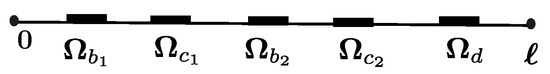
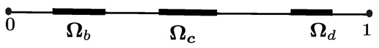
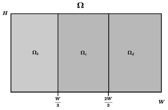
In Figure 2, we describe the domain geometry with the two scalar inputs and the two scalar outputs.

Figure 2. $\mathrm{\Omega }$, $n_b=2$, $n_c=2$.

Thus, we have $\mathcal{U}={\mathbb{R}}^{n_b}={\mathbb{R}}^2,\mathcal{Y}={\mathbb{R}}^{n_c}={\mathbb{R}}^2,\mathcal{D}={\mathbb{R}}^{n_d}=\mathbb{R},$ so that

$$B_{\mathrm{in}}u=b_1{u}_1+b_2{u}_2,b_j={{\displaystyle \chi }}_{{\mathrm{\Omega }}_{b_j}}\in \mathcal{Z},C\phi =\left[\begin{array}{c}{C}_1\phi \\ C_2\phi \end{array}\right]=\left[\begin{array}{c}⟨c_1,\phi ⟩\\ ⟨c_2,\phi ⟩\end{array}\right],c_j={{\displaystyle \chi }}_{{\mathrm{\Omega }}_{c_j}}\in \mathcal{Z},$$

(67)

and

$$G=C{(-A)}^{-1}{B}_{\mathrm{in}}={\left[⟨c_i,{(-A)}^{-1}{b}_j⟩\right]}_{i=1,j=1}^{2,2}.$$

(68)

We note that in this numerical simulation, with our choices of $b_j$ and $c_i$, the $2\times 2$ matrix G in (68) is invertible, $N\left(G^{*}\right)=\left\{0\right\}$, and the projection $L=0$.

In the system (65), we have set $a=2$, $v=2$ and set the length of the domain to $\ell =2$, so $\mathrm{\Omega }=[0,2]$. The sub-regions ${\mathrm{\Omega }}_{b_1}$, ${\mathrm{\Omega }}_{c_1}$, ${\mathrm{\Omega }}_{b_2}$, ${\mathrm{\Omega }}_{c_2}$, and ${\mathrm{\Omega }}_d$ are given by

$${\mathrm{\Omega }}_{b_1}=[0.25,0.35],{\mathrm{\Omega }}_{c_1}=[0.55,0.65],$$

$${\mathrm{\Omega }}_{b_2}=[0.85,0.95],{\mathrm{\Omega }}_{c_2}=[1.25,1.35],{\mathrm{\Omega }}_d=[1.55,1.65].$$

We have chosen asymptotic sinusoidal reference and disturbance signals with a smooth transition at time zero. Namely, we have set

$$r_1\left(t\right)=sin\left(t\right)F(t-2,1),r_2\left(t\right)=sin\left(2t\right)F(t-2,1),d\left(t\right)=cos\left(t\right)F(t-2,1),$$

(69)

where $F(t-t^{*},\epsilon )$ is a smooth, piecewise-defined unit step function centered at $t=t^{*}$. In the transition region $[t^{*}-\epsilon ,t^{*}+\epsilon ]$, F is a ninth-degree polynomial satisfying at the endpoints $t=t^{*}-\epsilon$ and $t=t^{*}+\epsilon$ the following: $F(-\epsilon ,\epsilon )=0$, $F(\epsilon ,\epsilon )=1$, and $F^{\left(k\right)}(-\epsilon ,\epsilon )=F^{\left(k\right)}(\epsilon ,\epsilon )=0$, $k=1,\dots ,4$. For $t<t^{*}-\epsilon$, we set $F=0$ and for $t>t^{*}+\epsilon$, we set $F=1$. The function F is introduced to suppress transient components that arise in the cascade iteration. These transient terms decay rapidly; F is included only to smooth the results in a neighborhood of $t=0$ without affecting the asymptotic behavior.

We solved three extra iterations for the cascade algorithm, producing errors $e_j$ via approximate controls $u^j$ for $j=0,1,2,3$. Therefore, we obtain the cumulative control, given by ${\displaystyle u_3=\sum _{j=0}^3{u}^j}$. The control $u=u_3$ was then applied in the plant

$$\begin{array}{cc}\hfill z_t=& Az+B_{\mathrm{d}}d+B_{\mathrm{in}}u,\hfill \end{array}$$

(70)

$$\begin{array}{cc}\hfill z(x,0)=& 2x(1-x),\hfill \end{array}$$

(71)

$$\begin{array}{cc}\hfill y\left(t\right)=& Cz=\left[\begin{array}{c}{C}_{1}z\\ C_{2}z\end{array}\right],\hfill \end{array}$$

(72)

where $C_1$ and $C_2$ are defined in (67). In our numerical simulation, we have set $\alpha ={10}^{-9}$, $\beta =0.25$ and computed three extra iterations.

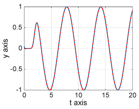
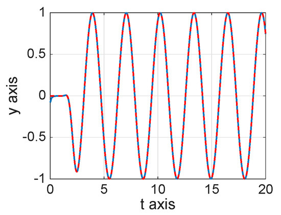
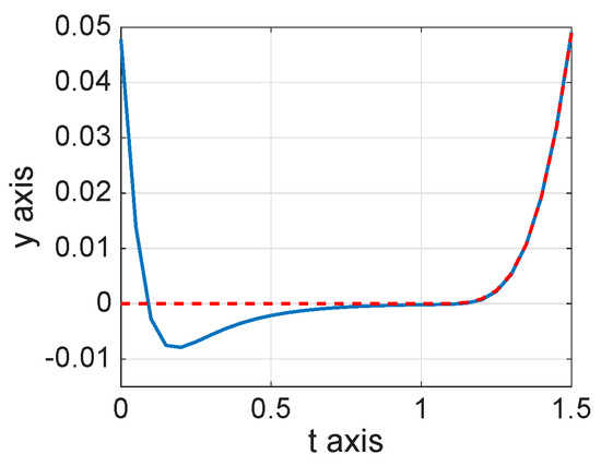
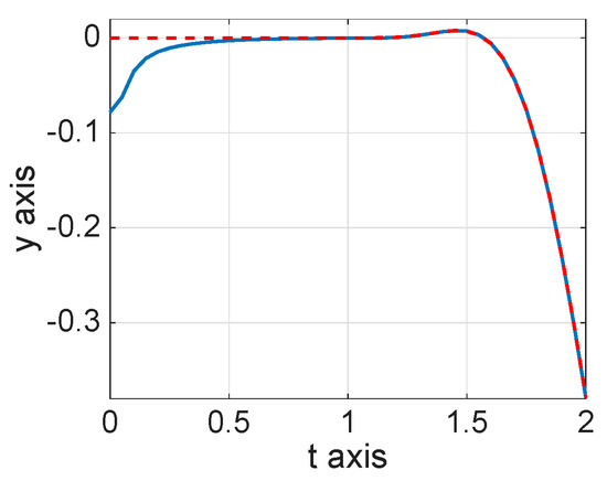
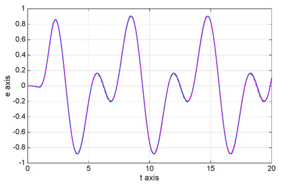
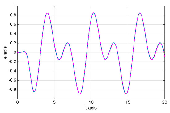
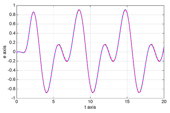
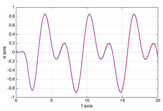
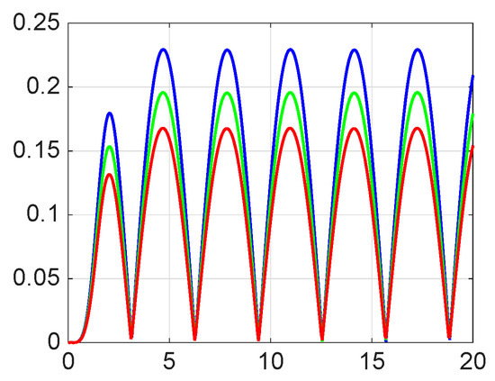
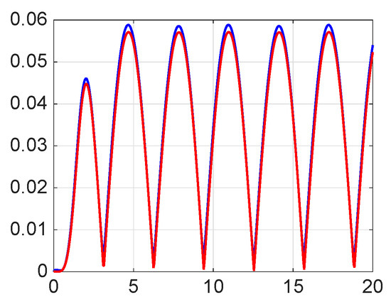
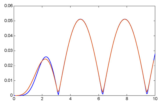
In Figure 3 and Figure 4, we have plotted the resulting numerical values obtained for $r_j\left(t\right)$ and $y_j\left(t\right)$ and notice that the curves are essentially indistinguishable after a very short time.

Figure 3. $y_1\left(t\right)$ (blue), $r_1\left(t\right)$ (red).

Figure 4. $y_2\left(t\right)$ (blue), $r_2\left(t\right)$ (red).

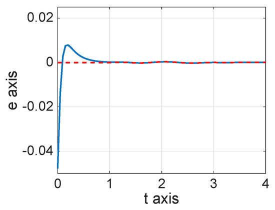
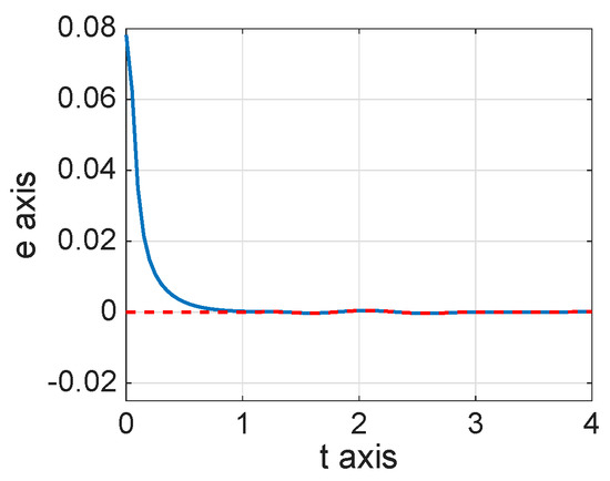
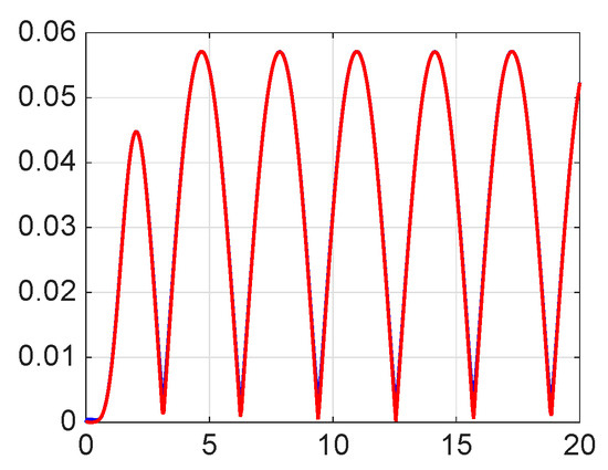
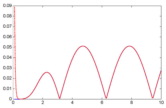
To draw attention to the rapid decay of the transient terms due to the nonzero initial conditions, in Figure 5 and Figure 6, we have plotted $r_j$ and $y_j$ for small t.

Figure 5. $y_1\left(t\right)$ (blue), $r_1\left(t\right)$ (red), for small time.

Figure 6. $y_2\left(t\right)$ (blue) and $r_2\left(t\right)$ (red) for small time.

Figure 7, Figure 8, Figure 9, Figure 10, Figure 11 and Figure 12 appear to demonstrate the rapid (even geometric) decrease to zero of the limsup of the errors to zero. In Table 1, we provide even stronger evidence by giving the ratios

$${\displaystyle \frac{\overline{\lim }\parallel e_{j1}\parallel }{\overline{\lim }\parallel e_{(j-1)1}\parallel }},{\displaystyle \frac{\overline{\lim }\parallel e_{j2}\parallel }{\overline{\lim }\parallel e_{(j-1)2}\parallel }}j=1,2,3.$$

Figure 7. $e_{01}\left(t\right)$ (blue), $e_{11}\left(t\right)$ (red).

Figure 8. $e_{11}\left(t\right)$ (blue), $e_{21}\left(t\right)$ (red).

Figure 9. $e_{21}\left(t\right)$ (blue), $e_{31}\left(t\right)$ (red).

Figure 10. $e_{02}\left(t\right)$ (blue), $e_{12}\left(t\right)$ (red).

Figure 11. $e_{12}\left(t\right)$ (blue), $e_{22}\left(t\right)$ (red).

Figure 12. $e_{22}\left(t\right)$ (blue), $e_{32}\left(t\right)$ (red).

Table 1. Comparison $\overline{\lim }\parallel e_{jk}\parallel /\overline{\lim }\parallel e_{(j-1)k}\parallel$ for $j=1,2,3$ and $k=1,2$.

	$\mathit{j}=1$	$\mathit{j}=2$	$\mathit{j}=3$
$k=1$	8.8800 × ${10}^{-2}$	1.0400 × ${10}^{-1}$	1.0060 × ${10}^{-1}$
$k=2$	8.6800 × ${10}^{-2}$	9.7800 × ${10}^{-2}$	9.8200 × ${10}^{-2}$

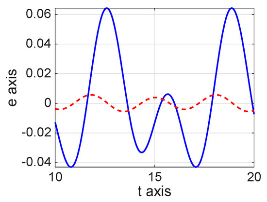
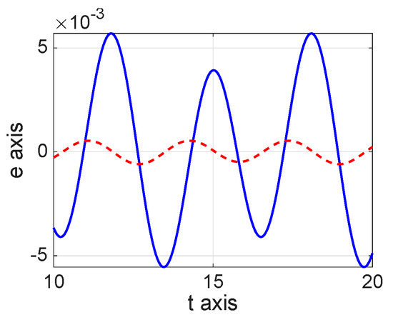
In Figure 13 and Figure 14, we draw attention to the errors from the cascade controller and the plant for small values of t. Namely, due to the difference in initial conditions for the controller and plant, we have a transient deviation in the first and second components of the plant error, $e_1$ and $e_2$, and the first and second components of the third cascade error, $e_{31}$ and $e_{32}$. Notice that these corresponding errors rapidly converge to each other.

Figure 13. $e_1\left(t\right)$ (blue), $e_{31}\left(t\right)$ (red).

Figure 14. $e_2\left(t\right)$ (blue), $e_{32}\left(t\right)$ (red).

Indeed, for this example, the $2\times 2$ transfer function G is invertible and the use of Tikhonov regularization or even Moore–Penrose pseudoinverse is not required to obtain an error-zeroing cascade control.

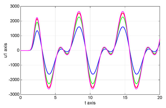
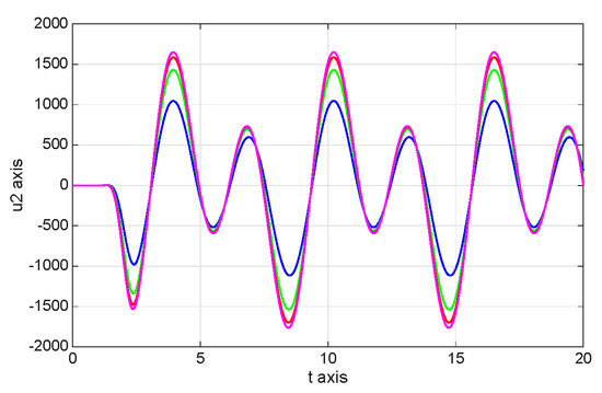
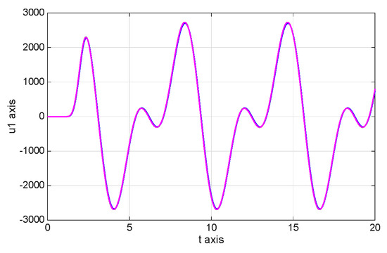
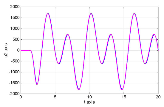
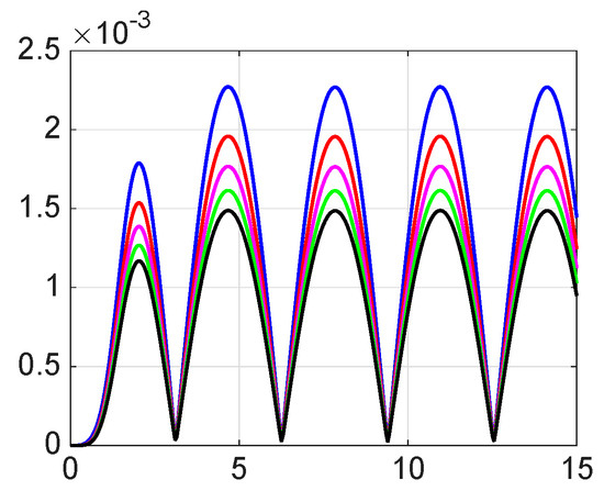
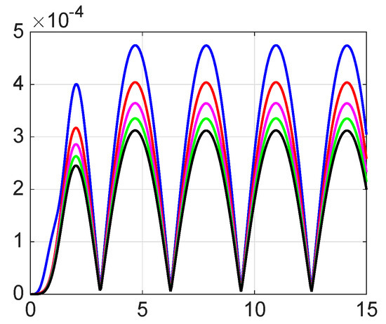
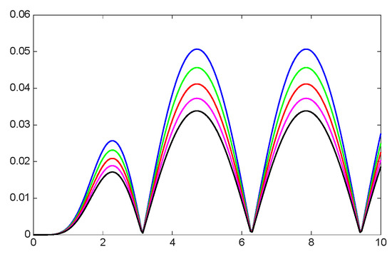
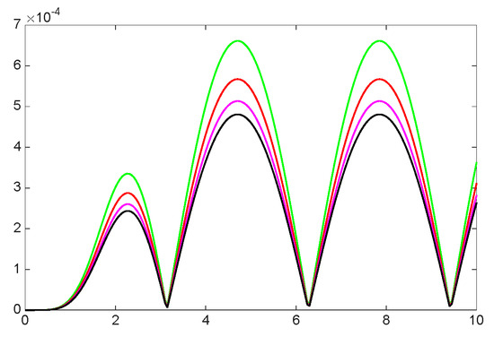
In order to demonstrate the convergence of the control $u_0=u^0$ in Equation (24), and the subsequent cascade controls $u_n={\sum }_{j=0}^n{u}^j$ in Equation (29), with the $u^j$ from Equation (28), we consider two values of the regularization parameter $\alpha ={10}^{-7},{10}^{-9}$. Each $u_n$, for $n=0,1,2,3$, consists of two components, denoted by $u_{n1}$ and $u_{n2}$. In Figure 15, corresponding to $\alpha ={10}^{-7}$, $u_{01}$ is shown in blue, $u_{11}$ in green, $u_{21}$ in red, and $u_{31}$ in magenta. Similarly, in Figure 16, $u_{02}$ is blue, $u_{12}$ is green, $u_{22}$ is red, and $u_{32}$ is magenta. The same color convention is used in Figure 17 and Figure 18, which corresponds to $\alpha ={10}^{-9}$. Note that for $\alpha ={10}^{-7}$, the cascade controls converge toward the optimal ones as n increases, but for the smaller value, $\alpha ={10}^{-9}$, the cascade controls essentially lie on top of each other.

Figure 15. $u_{j1}\left(t\right)$, with $j=0,1,2,3$, and $\alpha ={10}^{-7}$.

Figure 16. $u_{j2}\left(t\right)$, with $j=0,1,2,3$, and $\alpha ={10}^{-7}$.

Figure 17. $u_{j1}\left(t\right)$, with $j=0,1,2,3$, and $\alpha ={10}^{-9}$.

Figure 18. $u_{j2}\left(t\right)$, with $j=0,1,2,3$, and $\alpha ={10}^{-9}$.

Example 2

(${\mathit{n}}_{\mathit{b}}=\mathbf{1}$, ${\mathit{n}}_{\mathit{c}}=\mathbf{2}$). Our second simulation considers an under-determined system with one scalar input and two scalar outputs. Here, we use the same rod considered in the previous example, but in this case, we consider ${\mathrm{\Omega }}_b={\mathrm{\Omega }}_{b_1}\cup {\mathrm{\Omega }}_{b_2}$ (see Figure 2). In this case, we have $\mathcal{U}={\mathbb{R}}^{n_b}=\mathbb{R},\mathcal{Y}={\mathbb{R}}^{n_c}={\mathbb{R}}^2,\mathcal{D}={\mathbb{R}}^{n_d}=\mathbb{R}$ so that

$$B_{\mathrm{in}}u=bu,b={{\displaystyle \chi }}_{{\mathrm{\Omega }}_b}\in \mathcal{Z},C\phi =\left[\begin{array}{c}{C}_1\phi \\ C_2\phi \end{array}\right]=\left[\begin{array}{c}⟨c_1,\phi ⟩\\ ⟨c_2,\phi ⟩\end{array}\right],c_j\in \mathcal{Z}.$$

Remark 6. 

Unlike the previous example, in this case, G is a $2\times 1$ matrix, so not invertible, but, as we will see below, $G^{*}G$ is $1\times 1$ and invertible. Therefore, there is a well-defined Moore–Penrose pseudoinverse given by

$$G^{†}={\left(G^{*}G\right)}^{-1}{G}^{*},$$

so it would not be necessary to use Tikhonov regularization. Nevertheless, we provide the details of the development made in Section 3 and Section 4.

In this case, we have

$$G=C{(-A)}^{-1}{B}_{\mathrm{in}}=\left[\begin{array}{c}⟨c_1,{(-A)}^{-1}b⟩\\ ⟨c_2,{(-A)}^{-1}b⟩\end{array}\right]:=\left[\begin{array}{c}{\gamma }_1\\ {\gamma }_2\end{array}\right]G^{*}=\left[\begin{array}{cc}{\gamma }_1& {\gamma }_2\end{array}\right],$$

(73)

and

$$G^{*}G={\gamma }_1^2+{\gamma }_2^2:={\sigma }^2,{\sigma }_{\alpha }^2=\alpha +{\sigma }^2.$$

(74)

$$R_{\alpha }={(\alpha +G^{*}G)}^{-1}{G}^{*}={\displaystyle \frac{1}{{\sigma }_{\alpha }^2}}\left[\begin{array}{cc}{\gamma }_1& {\gamma }_2\end{array}\right]$$

(75)

Recall that

$$L_{\alpha }=I-G{R}_{\alpha }=I-G{(\alpha +G^{*}G)}^{-1}{G}^{*}=I-{(\alpha +G{G}^{*})}^{-1}G{G}^{*},$$

where ${\displaystyle G{G}^{*}={\left[{\gamma }_i{\gamma }_j\right]}_{i,j=1}^2}$. In this case, spectral analysis for the matrix $G{G}^{*}$ is straightforward. The eigenvalues are 0 and ${\sigma }^2$ and orthonormal eigenvectors are

$${\psi }_0={\displaystyle \frac{1}{\sigma }}\left[\begin{array}{c}{\gamma }_2\\ -{\gamma }_1\end{array}\right],{\psi }_1={\displaystyle \frac{1}{\sigma }}\left[\begin{array}{c}{\gamma }_1\\ {\gamma }_2\end{array}\right],$$

(76)

satisfying

$$G{G}^{*}{\psi }_0=0,G{G}^{*}{\psi }_1={\sigma }^2{\psi }_1,{⟨{\psi }_i,{\psi }_j⟩}_{{\mathbb{R}}^2}={\psi }_i{\psi }_j^{⊺}={\delta }_{i,j}.$$

Therefore,

$${(\alpha +G{G}^{*})}^{-1}G{G}^{*}={\displaystyle \frac{{\sigma }^2}{{\sigma }_{\alpha }^2}}{\psi }_1{\psi }_1^{⊺},$$

and, from (30)

$$\begin{array}{cc}\hfill L_{\alpha }=& I-{(\alpha +G{G}^{*})}^{-1}G{G}^{*}={\psi }_0{\psi }_0^{⊺}+{\psi }_1{\psi }_1^{⊺}-{\displaystyle \frac{{\sigma }^2}{{\sigma }_{\alpha }^2}}{\psi }_1{\psi }_1^{⊺},\hfill \\ \hfill =& {\psi }_0{\psi }_0^{⊺}+{\displaystyle \frac{\alpha }{{\sigma }_{\alpha }^2}}{\psi }_1{\psi }_1^{⊺}=L+M_{\alpha },\hfill \end{array}$$

where L and $M_{\alpha }$ are defined in (31), and in this case given explicitly by

$$L={\psi }_0{\psi }_0^{⊺},M_{\alpha }={\displaystyle \frac{\alpha }{{\sigma }_{\alpha }^2}}{\psi }_1{\psi }_1^{⊺},L{M}_{\alpha }=M_{\alpha }L=0.$$

(77)

Here, L is the orthogonal projection onto the $N\left(G{G}^{*}\right)$ and $\parallel M_{\alpha }\parallel$ goes to zero as $\alpha$ goes to zero. Finally, the operator $A_{\alpha ,\beta }$ is

$$A_{\alpha ,\beta }(·)=A(·)-{\displaystyle \frac{(1-\beta )b}{\alpha +\beta {\sigma }^2}}\left[{\gamma }_1⟨c_1,·⟩+{\gamma }_2⟨c_2,·⟩\right].$$

In this example, we have chosen the same reference and disturbance signals considered in (69) in Example 1. We note that in this case, while our controls are in some sense optimal, the tracking errors do not converge to zero. The point is that the control input does its best to track two different reference signals. In this example, the critical point of our work is that we can explain exactly what the errors are converging to as time goes to infinity.

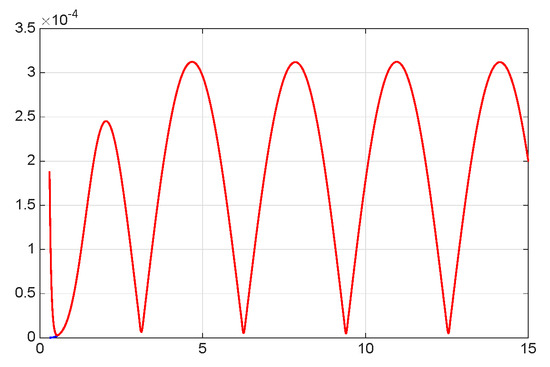
In Figure 19, we have set $\alpha ={10}^{-6}$ and $\beta =0.25$ and plotted $e_{j1}$ for $j=0,1,2,3$. Similarly, Figure 20 presents the corresponding results for $e_{j2}$ for $j=0,1,2,3$. We observe a slight variation in these curves due to the value of $\alpha$. To further investigate this effect, we decrease $\alpha$ to ${10}^{-9}$, obtaining the plots shown in Figure 21 and Figure 22. The curves are indistinguishable in this case, indicating that the earlier discrepancies resulted from the regularization parameter $\alpha$.

Figure 19. $e_{j1}$, $\alpha ={10}^{-6}$.

Figure 20. $e_{j2}\left(t\right)$, $\alpha ={10}^{-6}$.

Figure 21. $e_{j1}\left(t\right)$, $\alpha ={10}^{-9}$.

Figure 22. $e_{j2}\left(t\right)$, $\alpha ={10}^{-9}$.

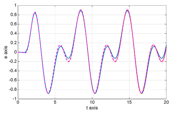
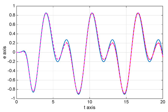
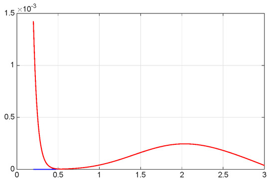
Figure 23 and Figure 24 contain plots of the components of the closed loop system error

$$e=\left[\begin{array}{c}{e}_1\\ e_2\end{array}\right]=r-C\left(z\right)$$

where z is the state variable obtained from the plant, (70)–(72), using the cascade control $u_3={\sum }_{j=0}^3{u}^j$ and the error formula $E_1$ obtained by sending $\alpha$ to zero as described in (42) and (43). Namely, we have

$$E_1\left(t\right):=\left[\begin{array}{c}{E}_{11}\\ E_{12}\end{array}\right]:=\underset{\alpha \to 0}{lim}{e}_1\left(t\right)=P\left(t\right)+L\left({\mathcal{H}}_0\left(t\right)+{\mathcal{H}}_1\left(t\right)\right)+{\mathcal{H}}_2\left(t\right).$$

We note that the term $P\left(t\right)$ decays to zero exponentially with time, and the term ${\mathcal{H}}_2\left(t\right)$ is very small compared with the term $L\left({\mathcal{H}}_0\left(t\right)+{\mathcal{H}}_1\left(t\right)\right)$. In particular, we observe that the main contribution to the error comes from the projection onto the $N\left(G^{*}\right)=R{\left(G\right)}^{\perp }$. Note that the two curves are on top of each other, confirming the accuracy of our explicit formula for the error.

Figure 23. $e_1\left(t\right)$ and $E_{11}\left(t\right)$, $\alpha ={10}^{-9}$.

Figure 24. $e_2\left(t\right)$ and $E_{12}\left(t\right)$, $\alpha ={10}^{-9}$.

Introduction of the function F in the definitions of r and d allows for the very smooth plots near $t=0$ in Figure 23 and Figure 24. Without it, there would be large oscillations from the exponentially decaying terms $P\left(t\right)$.

Example 3

(Non-Colocated Infinite-Dimensional Input and Output Spaces). In this example, we consider a control problem in one spatial dimension. We impose Dirichlet boundary conditions at the endpoints of the domain $\mathrm{\Omega }=[0,1]$. As in the previous examples, we write the state operator A for our plant as in (65).

As reported in Figure 25, here we take

$${\mathrm{\Omega }}_b=\left[{\displaystyle \frac{1}{5}},{\displaystyle \frac{2}{5}}\right],{\mathrm{\Omega }}_c=\left[{\displaystyle \frac{1}{2}},{\displaystyle \frac{7}{10}}\right],{\mathrm{\Omega }}_d=\left[{\displaystyle \frac{4}{5}},{\displaystyle \frac{9}{10}}\right],$$

so that we can write

$$B_{\mathrm{in}}={\mathcal{E}}_b,C={{\displaystyle \chi }}_{{\mathrm{\Omega }}_c}\left(x\right),\mathrm{and}{B}_{\mathrm{d}}\left(x\right)={\mathcal{E}}_d.$$

Figure 25. One-dimensional rod, non-colocated.

Here, we have noted that the restriction operator can be explicitly expressed in terms of the characteristic function so we can write

$$C\psi \left(x\right)={\mathcal{R}}_c\psi \left(x\right)={{\displaystyle \chi }}_{{\mathrm{\Omega }}_c}\psi \left(x\right).$$

Therefore, in this example, the input operator is an extension operator, and the output operator is a restriction operator. We consider a tracking problem with reference and disturbance signals

$$r(x,t)=xsin\left(t\right)F(t-1.5,1.5),d(x,t)=x^{2}sin\left(2t\right)F(t-1.5,1.5)$$

(78)

where F is a smooth function that, together with its first four derivatives, is zero at $t=0$. The function F is introduced to suppress transient terms that arise in the cascade iteration. These transient terms decay exponentially in time.

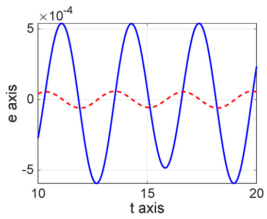
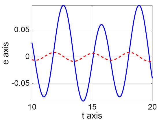
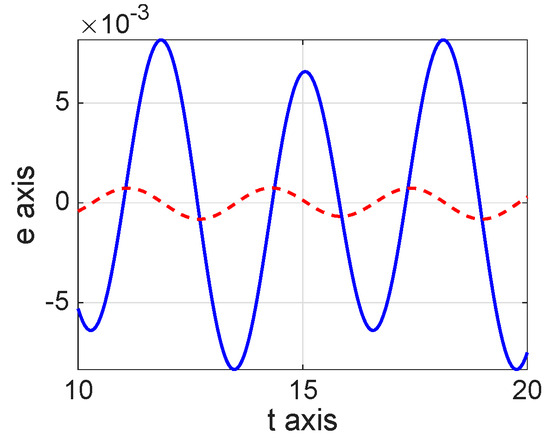
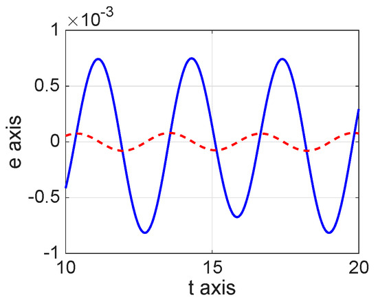
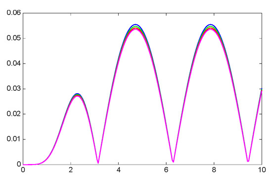
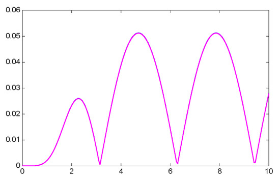
In this case, the resulting controls obtained at each cascade step are functions of both x and t. In Figure 26, Figure 27, Figure 28 and Figure 29, we have plotted the norms $\parallel e_j{\parallel }_c$ of the errors $e_j$ for $j=0,1,2$ and for $\alpha ={10}^{-3},{10}^{-5},{10}^{-7},{10}^{-9}$. Here, we have used blue to depict $e_0$, green for $e_1$, and red for $e_2$.

Figure 26. $\parallel e_j{\parallel }_c$$j=0,1,2$, $\alpha ={10}^{-3}$.

Figure 27. $\parallel e_j{\parallel }_c$$j=0,1,2$, $\alpha ={10}^{-5}$.

Figure 28. $\parallel e_j{\parallel }_c$$j=0,1,2$, $\alpha ={10}^{-7}$.

Figure 29. $\parallel e_j{\parallel }_c$$j=0,1,2$, $\alpha ={10}^{-9}$.

In the above figures, we used the following color code to indicate the curves $\parallel e_j\left(t\right)\parallel$: $\parallel e_0\left(t\right)\parallel$ blue, $\parallel e_1\left(t\right)\parallel$ green, and $\parallel e_2\left(t\right)\parallel$ red.

The main point here is that for $\alpha <{10}^{-5}$, the errors converge very rapidly to a limiting function, which is that given by the sum of the formulas given in (38) for $e_n^r$ and (39) for $e_n^d$. In particular, we note that as $\alpha$ becomes small, the contributions from $M_{\alpha }$ become negligible very quickly, and the main contribution is from the projection L onto the null space of $G^{*}$.

Once again, after two iterations of the cascade algorithm, we obtain the cumulative control, given by ${\displaystyle u_2=\sum _{j=0}^2{u}^j}$. The control $u=u_2$ was then applied in the plant

$$\begin{array}{cc}\hfill z_t=& Az+B_{\mathrm{d}}d+B_{\mathrm{in}}u,\hfill \end{array}$$

(79)

$$\begin{array}{cc}\hfill z(x,0)=& x(1-x),\hfill \end{array}$$

(80)

$$\begin{array}{cc}\hfill y\left(t\right)=& Cz,\hfill \end{array}$$

(81)

producing the error $e(x,t)=r(x,t)-Cz(x,t)$ with norm

$${\parallel e\left(t\right)\parallel }_c={\left({\int }_{{\mathrm{\Omega }}_c}{|r(x,t)-Cz(x,t)|}^{2}dx\right)}^{1/2}.$$

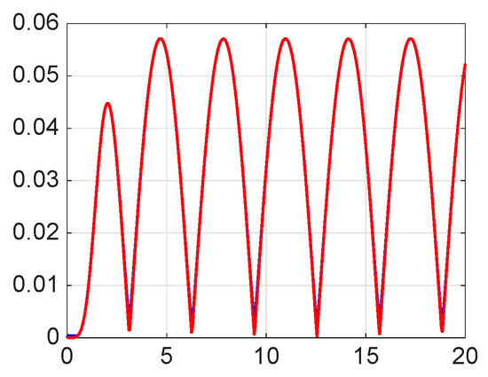
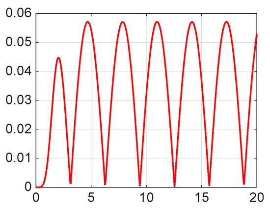
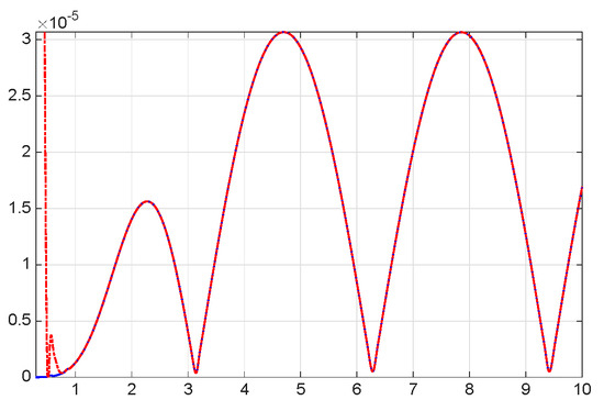
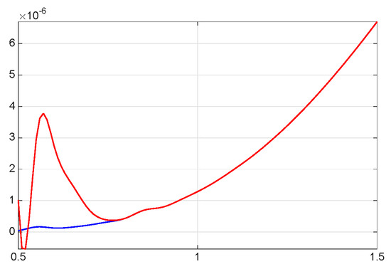
In Figure 30 and Figure 31, we have plotted the norm of plant system error $e\left(t\right)$ (in red) and, just as in the previous example, the first approximate error $E_0$ (in blue) given by the formulas in (38) and (39). Notice that in the case of infinite-dimensional input and output spaces, we cannot use the formulas described in (42) and (43) since $M_{\alpha }$ becomes unbounded as $\alpha$ goes to zero in the operator norm; however, it does go to zero in the strong operator topology.

Figure 30. $\parallel E_0{\parallel }_c$, ${\parallel e\parallel }_c$, $\alpha ={10}^{-9}$.

Figure 31. Same for small t.

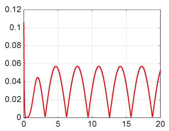
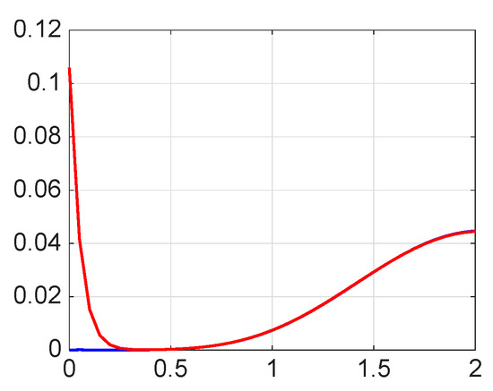
In Figure 32 and Figure 33, we have plotted $\parallel e_2{\left(t\right)\parallel }_c$ (in blue) for $\alpha ={10}^{-9}$ obtained by solving our cascade control algorithm along with the norm of the error, $E_{\mathrm{oc}}$ (in red), obtained by computing an optimal control u using the variational approach formulation in (82)–(84) with $ϵ={10}^{-9}$. We notice that the two curves are indistinguishable.

Figure 32. $\parallel E_{\mathrm{oc}}{\parallel }_c$ and $\parallel e_2{\left(t\right)\parallel }_c$ with $ϵ=\alpha ={10}^{-9}$.

Figure 33. Same for small t.

Here, the “full control” u is obtained by using minimizing variations for the form

$$J_{ϵ}(r,z,d,u)={\int }_0^T\left[{\int }_{{\mathrm{\Omega }}_c}{\displaystyle \frac{1}{2}}{(z-r)}^{2}dx+{\displaystyle \frac{ϵ}{2}}{\int }_{{\mathrm{\Omega }}_b}{u}^{2}dx+{\int }_{\mathrm{\Omega }}\lambda \left(z_t-Az-B_{\mathrm{in}}u-B_{\mathrm{d}}d\right)dx\right]dt$$

with appropriate boundary conditions on z and $\lambda$. This analysis leads to the following system:

$$\begin{array}{cc}\hfill {\overline{z}}_t& =A\overline{z}+B_{\mathrm{d}}d+B_{\mathrm{in}}\left({\displaystyle \frac{-\lambda }{ϵ}}\right),\hfill \end{array}$$

(82)

$$\begin{array}{cc}\hfill -{\lambda }_t& =A^{*}+{{\displaystyle \chi }}_{{\mathrm{\Omega }}_c}(r-\overline{z}),\hfill \end{array}$$

(83)

$$\begin{array}{cc}\hfill \overline{z}(0,t)& =\overline{z}(L,t)=\lambda (0,t)=\lambda (L,t)=\lambda (x,T)=0.\hfill \end{array}$$

(84)

The desired control law is

$$u={\displaystyle \frac{-\lambda }{ϵ}}.$$

Note that Equation (83) is an inverse parabolic equation with initial data prescribed at T and must therefore be integrated backward in time (from T to 0). Consequently, the optimality system (82)–(84) must be solved all at once on the full interval $[0,T]$, effectively coupling time as an additional dimension of the discrete problem and making the control solve substantially more demanding.

COMSOL, however, is engineered for classical time marching, not for globally coupled space–time solves. To approximate (82)–(84), we adopted a workaround, embedding the PDE in a cylindrical domain with an auxiliary coordinate that mimics time. While feasible, this reformulation is markedly more expensive (many time levels are coupled simultaneously), scales poorly with problem size, and is not practical in 3D. For these reasons, a head-to-head runtime comparison would be misleading: any timings would reflect COMSOL’s solver limitations for all-at-once optimal control rather than the intrinsic efficiency of the methods. Specialized software [33], by contrast, implements forward–backward (sweep) iterations until convergence [17,18], yielding faster solves of (82)–(84) and making such approaches competitive. However, this lies outside the scope of the present work, so we omit any runtime comparisons between the two methods.

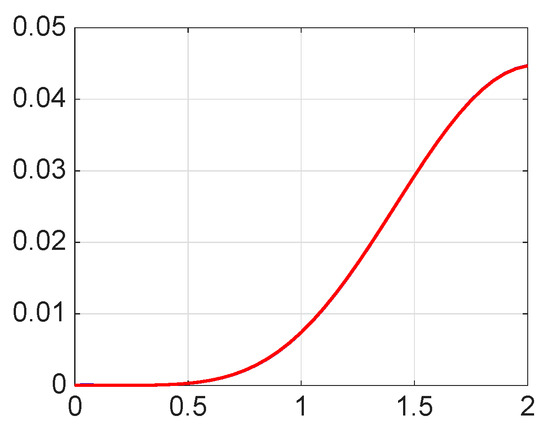
Example 4

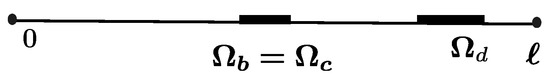
(Colocated Infinite-Dimensional Input and Output Spaces). In this example, we consider the same system operator A introduced at the beginning of this section in (65) with domain (66) where $\mathrm{\Omega }=[0,\ell ]$. The main difference between Example 3 and this example is that we consider a colocated case in which ${\mathrm{\Omega }}_b={\mathrm{\Omega }}_c$, see Figure 34. In this case, we expect the norms of the errors obtained from the cascade algorithm to decrease geometrically because of Lemma 3.

Figure 34. One-dimensional rod, colocated.

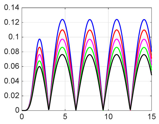
In our simulation, we have chosen $\ell =1$, ${\mathrm{\Omega }}_b={\mathrm{\Omega }}_c=[0.45,0.55]$, and ${\mathrm{\Omega }}_d=[0.7,0.8]$. We have run five additional steps in our cascade using the same r and d introduced in (78). In Figure 35, Figure 36, Figure 37, Figure 38 and Figure 39, we have plotted $\parallel e_j{\parallel }_c$ for $j=1,2,3,4,5$ for $\alpha ={10}^{-3},{10}^{-5},{10}^{-7},{10}^{-9}$, respectively. As expected, and unlike the previous example, the error norms decrease geometrically with each iteration.

Figure 35. $\parallel e_j{\parallel }_c$$j=1,\dots ,5$, $\alpha ={10}^{-3}$.

Figure 36. $\parallel e_j{\parallel }_c$$j=1,\dots ,5$, $\alpha ={10}^{-5}$.

Figure 37. $\parallel e_j{\parallel }_c$$j=1,\dots ,5$, $\alpha ={10}^{-7}$.

Figure 38. $\parallel e_j{\parallel }_c$$j=1,\dots ,5$, $\alpha ={10}^{-9}$.

Figure 39. $\parallel e_5{\left(t\right)\parallel }_c$ (blue) $e\left(t\right)$, (red) $\alpha ={10}^{-9}$.

In the above figures, we used the following color code to indicate the curves $\parallel e_j\left(t\right)\parallel$: $\parallel e_1\left(t\right)\parallel$ blue, $\parallel e_2\left(t\right)\parallel$ red, $\parallel e_3\left(t\right)\parallel$ magenta, $\parallel e_4\left(t\right)\parallel$ green, and $\parallel e_5\left(t\right)\parallel$ black. Then, in Figure 39 and Figure 40, we have set $\alpha ={10}^{-9}$ and plotted both $\parallel e_5{\parallel }_c$ and the norm of the plant system error, ${\parallel e\left(t\right)\parallel }_c={\parallel r\left(t\right)-z\left(t\right)\parallel }_c$, where we have used the control ${\displaystyle u_5=\sum _{j=0}^5{u}^j}$. After a very short transient, the two curves are indistinguishable.

Figure 40. $\parallel e_5{\parallel }_c$ (blue) and ${\parallel e\left(t\right)\parallel }_c$ (red) for small t.

Figure 35, Figure 36 and Figure 37 demonstrate a geometric decrease in the limsup of the errors. In Table 2, we provide even stronger evidence by giving the ratios

$${\displaystyle \frac{\overline{\lim }\parallel e_j\parallel }{\overline{\lim }\parallel e_{(j-1)}\parallel }},j=1,\dots ,5.$$

Table 2. $\overline{\lim }\parallel e_j\parallel /\overline{\lim }\parallel e_{(j-1)}\parallel$ for $j=1,\dots ,5$ and $\alpha ={10}^{-k}k=3,5,7,9$.

	$\mathit{\alpha }={10}^{-3}$	$\mathit{\alpha }={10}^{-5}$	$\mathit{\alpha }={10}^{-7}$	$\mathit{\alpha }={10}^{-9}$
$j=1$	0.8851	0.5238	0.6486	0.1369
$j=2$	0.8852	0.9765	0.8622	0.8516
$j=3$	0.8854	0.9817	0.9024	0.9014
$j=4$	0.8856	0.9818	0.9137	0.9202
$j=5$	0.8858	0.9820	0.9215	0.9315

We note that for each value of $\alpha$, the ratios of ${\displaystyle \frac{\overline{\lim }\parallel e_1\parallel }{\overline{\lim }\parallel e_0\parallel }}$ are significantly smaller than all the subsequent ratios, so the first step in the iterative scheme always produces an outlier in the geometric convergence. In the following table, we confirm the above statement by providing the ratios of the limsups of the norms of the errors pairwise.

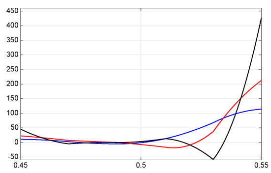
Figure 41 plots the cascade control $u_5(x,t)={\sum }_{j=0}^5{u}^j(x,t)$ at the final time $t=15$, for three values of $\alpha ={10}^{-7}$, ${10}^{-8}$, and ${10}^{-9}$, over the domain ${\mathrm{\Omega }}_b$. The curves $u_5(x,15)$ are colored blue for $\alpha ={10}^{-7}$, red for $\alpha ={10}^{-8}$, and black for $\alpha ={10}^{-9}$. As $\alpha$ decreases, the control becomes progressively rougher, reflecting higher-frequency oscillations that enhance tracking accuracy. Conversely, for larger values of $\alpha$, the control smooths out and approaches an almost constant profile.

Figure 41. $u_5(x,15)$ for $\alpha ={10}^{-7}$ (blue), ${10}^{-8}$ (red), and ${10}^{-9}$ (black).

Example 5

(Non-Colocated Example in a Two-Dimensional Spatial Domain). We consider a control problem in two spatial dimensions analogous to the one-dimensional Example 3. In this example, we again impose Dirichlet boundary conditions on the boundary of a domain $\mathrm{\Omega }\subset {\mathbb{R}}^2$ (see Figure 42). We can write the state operator for our plant as

$$\begin{array}{cc}\hfill A=& a\Delta -V·\mathrm{grad},V=[u,v]\hfill \\ \hfill D\left(A\right)& =\{\phi \in H^2\left(\mathrm{\Omega }\right):\phi {|}_{\partial \mathrm{\Omega }}=0\}.\hfill \end{array}$$

(85)

Figure 42. Two-dimensional region, non-colocated.

As in our previous examples, the operator A is not self-adjoint. Rather, we have

$$A^{*}=a\Delta +V·\mathrm{grad}$$

with

$$D\left(A^{*}\right)=\{\phi \in H^2\left(\mathrm{\Omega }\right):\phi {|}_{\partial \mathrm{\Omega }}=0\}.$$

We consider a tracking problem with reference and disturbance signals

$$\begin{array}{cc}\hfill r(x,y,t)=& xy(1-y)(y-0.5)sin\left(t\right)F(t-1.5,1.5),\hfill \end{array}$$

(86)

$$\begin{array}{cc}\hfill d(x,y,t)=& x{(y-0.5)}^{2}sin\left(2t\right)F(t-1.5,1.5),\hfill \end{array}$$

(87)

where, as in the previous example, F is a smooth function that, together with its first four derivatives, is zero in a neighborhood of $t=0$. The function F is introduced to suppress transient terms that arise in the cascade iteration. These transient terms decay exponentially in time.

In this case, the resulting cascade controls $u^j$, the cascade control, $u_n={\sum }_{j=0}^n{u}^j$, and the full optimal control are functions of both x, y and t.

For comparison, in this example, we have also solved a system similar to (82)–(84) to obtain an optimal control using an inverse parabolic equation for the Lagrange multiplier $\lambda$. The error associated with this control is denoted by $E_{oc}\left(t\right)$. Also, the error obtained when using the cascade control $u_3$ in the plant with initial condition $\phi \left(x\right)=xy$ is denoted by $e\left(t\right)$.

For our simulations, we have set $a=2$, $u=v=2$, $\beta =0.25$ and taken various values for $\alpha$. In this case, just as in Example 3, for small $\alpha$, the dynamics are dominated by the projection onto the $N\left(G^{*}\right)$. For that reason, in Figure 43, we have plotted the results for a large value of $\alpha ={10}^{-4}$ to demonstrate the decrease in the norm for the errors $\parallel e_j{\parallel }_c$ for $j=0,1,2,3$. Then, in Figure 44, Figure 45 and Figure 46, we have fixed $\alpha ={10}^{-7}$. In Figure 44, we have again plotted the norm for the errors $\parallel e_j{\parallel }_c$ for $j=0,1,2,3$. In this case, the different curves are indistinguishable for all t. In Figure 45, we plotted the norms of the cascade error $e_3$ and the plant error using nonzero initial data. Finally, in Figure 46, we compare the cascade error $e_3$ and the full optimal control error $E_{\mathrm{oc}}$ obtained with the penalty constant $ϵ={10}^{-7}$. After a short transient, the two errors become indistinguishable.

Figure 43. $\parallel e_j{\parallel }_c$$j=0,\dots ,3$, $\alpha ={10}^{-4}$.

Figure 44. $\parallel e_j{\parallel }_c$$j=0,\dots ,3$, $\alpha ={10}^{-7}$.

Figure 45. $\parallel e_3{\parallel }_c$, ${\parallel e\parallel }_c$, $\alpha ={10}^{-9}$.

Figure 46. $\parallel e_3{\parallel }_c$, $\parallel E_{\mathrm{oc}}{\parallel }_c$.

Example 6

(Colocated Example in a Two-Dimensional Spatial Domain). This example considers a control problem in two spatial dimensions analogous to the one-dimensional colocated Example 4. Namely, we assume that the equations, reference and disturbance signals, and basic geometry are the same as in Example 5 except that now we assume that ${\mathrm{\Omega }}_b$ and ${\mathrm{\Omega }}_c$ are colocated (see Figure 47). In this case, we expect the cascade controls to produce errors that go to zero geometrically with increasing cascade iterations. Once again, impose Dirichlet boundary conditions on the boundary of a domain $\mathrm{\Omega }\subset {\mathbb{R}}^2$.

Figure 47. Two-dimensional region, colocated.

In our numerical simulations, we have computed the cascade errors $e_j$ for $j=0,\dots ,3$ for various values of $\alpha$. In Figure 48, we have plotted $\parallel e_j{\left(t\right)\parallel }_c$ for $j=0,\dots ,3$ for $\alpha ={10}^{-4}$, and in Figure 49, we have plotted these same results for $\alpha ={10}^{-7}$. Notice that, for fixed $\alpha$, the norms decrease geometrically with each cascade iteration.

Figure 48. $\parallel e_j{\parallel }_c$$j=0,\dots ,4$, $\alpha ={10}^{-4}$.

Figure 49. $\parallel e_j{\parallel }_c$$j=1,\dots ,4$, $\alpha ={10}^{-7}$.

In the above figures, we used the following color code to indicate the curves $\parallel e_j\left(t\right)\parallel$: $\parallel e_0\left(t\right)\parallel$ blue, $\parallel e_1\left(t\right)\parallel$ green, $\parallel e_2\left(t\right)\parallel$ red, $\parallel e_3\left(t\right)\parallel$ magenta, and $\parallel e_5\left(t\right)\parallel$ black. In Figure 50 and Figure 51, we have plotted the $\parallel e_4{\left(t\right)\parallel }_c$ and the norm of the plant error ${\parallel e\left(t\right)\parallel }_c$ both for large and small times. Here, we have set the initial condition for the plant to $\phi \left(x\right)=xy$. Notice that after a very brief time, the two curves become indistinguishable.

Figure 50. $\parallel e_4{\parallel }_c$, ${\parallel e\parallel }_c$, $\alpha ={10}^{-9}$.

Figure 51. $\parallel e_4{\parallel }_c$, ${\parallel e\parallel }_c$ on $0.5<t<1.5$.

9. Conclusions

This work introduces a rigorous and general methodology for achieving asymptotic tracking and disturbance rejection in both lumped and distributed parameter systems, including those with infinite-dimensional input and output spaces. We overcome significant challenges posed by compact operators in infinite-dimensional input and output spaces by employing a cascade algorithm based on the geometric regulation theory, which is enhanced with Tikhonov regularization. Our approach extends beyond traditional optimal control methods, providing approximate solutions for various systems, including those that are over- or under-determined.

Through a detailed error analysis, we identify conditions under which the cascade process is error zeroing and those that limit its effectiveness, such as non-colocated input–output operators and contributions from regularization. Numerical simulations validate the method’s practical applicability, demonstrating its adaptability across diverse examples with varying dimensionality and configurations. This study lays a foundation for further research into advanced control strategies for complex linear and nonlinear dynamical systems control, with potential extensions to unbounded input and output operators and broader classes of nonlinear partial differential equations.

References

- Aulisa, E.; Gilliam, D. A Practical Guide to Geometric Regulation for Distributed Parameter Systems; CRC Press: Boca Raton, FL, USA, 2015. [Google Scholar]
- Burns, J.A.; He, X.; Hu, W. Feedback stabilization of a thermal fluid system with mixed boundary control. Comput. Math. Appl. 2016, 71, 2170–2191. [Google Scholar] [CrossRef]
- Deutscher, J.; Kerschbaum, S. Robust output regulation by state feedback control for coupled linear parabolic PIDEs. IEEE Trans. Autom. Control 2019, 65, 2207–2214. [Google Scholar] [CrossRef]
- Aulisa, E.; Gilliam, D.; Pathiranage, T. Analysis of an iterative scheme for approximate regulation for nonlinear systems. Int. J. Robust Nonlinear Control 2018, 28, 3140–3173. [Google Scholar] [CrossRef]
- Aulisa, E.; Gilliam, D.S.; Pathiranage, T.W. Analysis of the error in an iterative algorithm for asymptotic regulation of linear distributed parameter control systems. ESAIM Math. Model. Numer. Anal. 2019, 53, 1577–1606. [Google Scholar] [CrossRef]
- Aulisa, E.; Gilliam, D.S. Approximation methods for geometric regulation. arXiv 2021, arXiv:2102.06196. [Google Scholar]
- Francis, B.A.; Wonham, W.M. The internal model principle of control theory. Automatica 1976, 12, 457–465. [Google Scholar] [CrossRef]
- Francis, B.A. The linear multivariable regulator problem. SIAM J. Control Optim. 1977, 15, 486–505. [Google Scholar] [CrossRef]
- Hespanha, J.P. Linear Systems Theory, 2nd ed.; Princeton University Press: Princeton, NJ, USA, 2018. [Google Scholar]
- Azimi, A.; Koch, S.; Reichhartinger, M. Robust internal model-based control for linear-time-invariant systems. Int. J. Robust Nonlinear Control 2024, 34, 12476–12496. [Google Scholar] [CrossRef]
- Bymes, C.I.; Laukó, I.G.; Gilliam, D.S.; Shubov, V.I. Output regulation for linear distributed parameter systems. IEEE Trans. Autom. Control 2000, 45, 2236–2252. [Google Scholar] [CrossRef]
- Anderson, B.D.; Moore, J.B. Optimal Control: Linear Quadratic Methods, reprint edition ed.; Dover Publications: Mineola, NY, USA, 2007. [Google Scholar]
- Dorato, P.; Abdallah, C.; Cerone, V. Linear-Quadratic Control: An Introduction; Krieger Publishing Company: Malabar, FL, USA, 2000. [Google Scholar]
- Najafi Birgani, S.; Moaveni, B.; Khaki-Sedigh, A. Infinite horizon linear quadratic tracking problem: A discounted cost function approach. Optim. Control Appl. Methods 2018, 39, 1549–1572. [Google Scholar] [CrossRef]
- Bornemann, F.A. An adaptive multilevel approach to parabolic equations III. 2D error estimation and multilevel preconditioning. IMPACT Comput. Sci. Eng. 1992, 4, 1–45. [Google Scholar] [CrossRef]
- Tröltzsch, F. On the Lagrange–Newton–SQP method for the optimal control of semilinear parabolic equations. SIAM J. Control Optim. 1999, 38, 294–312. [Google Scholar] [CrossRef]
- McAsey, M.; Mou, L.; Han, W. Convergence of the forward-backward sweep method in optimal control. Comput. Optim. Appl. 2012, 53, 207–226. [Google Scholar] [CrossRef]
- Tröltzsch, F. Optimal Control of Partial Differential Equations: Theory, Methods and Applications; Graduate Studies in Mathematics; American Mathematical Society: Providence, RI, USA, 2010; Volume 112. [Google Scholar]
- Lee, Y.; Kouvaritakis, B. Constrained receding horizon predictive control for systems with disturbances. Int. J. Control 1999, 72, 1027–1032. [Google Scholar] [CrossRef]
- Camacho, E.F.; Bordons, C. Constrained model predictive control. In Model Predictive Control; Springer: Berlin/Heidelberg, Germany, 2007; pp. 177–216. [Google Scholar]
- Güttel, S.; Pearson, J.W. A rational deferred correction approach to parabolic optimal control problems. IMA J. Numer. Anal. 2018, 38, 1861–1892. [Google Scholar] [CrossRef]
- Leveque, S.; Pearson, J.W. Fast iterative solver for the optimal control of time-dependent PDEs with Crank–Nicolson discretization in time. Numer. Linear Algebra Appl. 2022, 29, e2419. [Google Scholar] [CrossRef]
- Aulisa, E.; Burns, J.A.; Gilliam, D.S. Approximate Error Feedback Controller for Tracking and Disturbance Rejection for Linear Distributed Parameter Systems. In Proceedings of the 2022 American Control Conference (ACC), Atlanta, GA, USA, 8–10 June 2022; pp. 976–981. [Google Scholar]
- Conway, J.B. A Course in Functional Analysis; Springer: Berlin/Heidelberg, Germany, 2019; Volume 96. [Google Scholar]
- Kato, T. Perturbation Theory for Linear Operators; Springer Science & Business Media: Berlin/Heidelberg, Germany, 2013; Volume 132. [Google Scholar]
- Baumeister, J. Stable Solution of Inverse Problems; Springer: Berlin/Heidelberg, Germany, 1987. [Google Scholar]
- Kirsch, A. An Introduction to the Mathematical Theory of Inverse Problems, 3rd ed.; Applied Mathematical Sciences; Springer: Cham, Switzerland, 2021; Volume 120. [Google Scholar] [CrossRef]
- Morozov, V.A. Methods for Solving Incorrectly Posed Problems; Springer Science & Business Media: Berlin/Heidelberg, Germany, 2012. [Google Scholar]
- Kress, R.; Maz’ya, V.; Kozlov, V. Linear Integral Equations; Springer: Berlin/Heidelberg, Germany, 1989; Volume 82. [Google Scholar]
- Hsiao, G.C.; Wendland, W.L. Boundary Integral Equations, 2nd ed.; Applied Mathematical Sciences; Springer: Cham, Switzerland, 2021; Volume 164. [Google Scholar] [CrossRef]
- Fallahnejad, M.; Kazemy, A.; Shafiee, M. Event-triggered H∞ stabilization of networked cascade control systems under periodic DoS attack: A switching approach. Int. J. Electr. Power Energy Syst. 2023, 153, 109278. [Google Scholar] [CrossRef]
- Du, Z.; Chen, C.; Li, C.; Yang, X.; Li, J. Fault-Tolerant H-Infinity Stabilization for Networked Cascade Control Systems with Novel Adaptive Event-Triggered Mechanism. IEEE Trans. Autom. Sci. Eng. 2025. early access. [Google Scholar] [CrossRef]
- Hecht, F.; Lance, G.; Trélat, E. PDE-Constrained Optimization Within FreeFEM; Open-Access Monograph; LJLL/Sorbonne Université: Paris, France, 2024. [Google Scholar]
- Schwartz, J.T. Linear Operators: Spectral Theory: Self Adjoint Operators in Hilbert Space; Interscience: Saint-Nom-la-Bretéche, France, 1963. [Google Scholar]
- Lewin, M. Spectral Theory and Quantum Mechanics; Universitext; Springer: Cham, Switzerland, 2024. [Google Scholar] [CrossRef]
Disclaimer/Publisher’s Note: The statements, opinions and data contained in all publications are solely those of the individual author(s) and contributor(s) and not of MDPI and/or the editor(s). MDPI and/or the editor(s) disclaim responsibility for any injury to people or property resulting from any ideas, methods, instructions or products referred to in the content. |
© 2025 by the authors. Licensee MDPI, Basel, Switzerland. This article is an open access article distributed under the terms and conditions of the Creative Commons Attribution (CC BY) license (https://creativecommons.org/licenses/by/4.0/).